TítuloDo Government Revenues Matter for Economic Growth? Evidence from Nigeria
25
0
0
Texto completo
(2) Isiaka Akande Raifu and Abiodun Najeem Raheem / European Journal of Government and Economics 7(1), 60-84.. decline in the price of crude oil in mid-2014 has resulted in falling government revenues with socioeconomic consequences. This has become a burning issue in Nigeria. To reduce these socioeconomic malaises, the current government is determined to diversify the economy away from the exploration, production and export of crude oil to other sectors of the economy, particularly to the neglected or abandoned agricultural sector and the non-exploited mining subsector. 2 Specifically, the prices of crude oil fell from about $114 per barrel in 2014 to about $50 per barrel in recent time. The fall in the crude oil price has resulted in fall in government revenues, which has thwarted the efforts of governments both at local, state and national levels to finance their developmental projects and to fulfil other mandated responsibilities. This is because the country as a whole depends almost entirely on the oil revenues to finance its developmental projects. This has degenerated into many socio-economic crises such as nonpayment of workers’ salaries, weak demand for industrial products, closing of factories and retrenchment of workers, a high rate of serious crimes and overall decline in the aggregate economy. Moreover, oil revenue is not the only source of government revenue in Nigeria. Part of government revenues are also obtained from the agricultural sector, manufacturing subsector, service sector and other sectors of the economy. The revenues from these sectors come in different forms such as sales, taxes, fines, levies and tariffs. These revenues are referred to as non-oil revenue. Even though the non-oil revenue is small compared to oil revenue, it has been parts of the funds being used by government for the execution of both recurrent and capital projects. Historically, efforts at generating more revenues from other sources to complement oil revenue have seen the evolvement of different tax reforms, ranging from tax reform system employed before and during the colonial era to the automated tax system (Taxpayer’s Identification Number). In the course of these tax reforms, different tax methods have been adopted ranging from income tax, company tax, petroleum tax, capital gains tax, as well as value added tax introduced in 1994 (Odusola, 2006). However, the porosity in tax collection, which gives room to either tax avoidance or tax evasion has undermined the important contribution of taxes to economic growth, causing overreliance on oil revenue as a major source of financing government’s project apart from borrowing. As noted before, the volatility in oil price often results in revenue volatility, expenditure volatility, output volatility and unstable or unsustainable economic growth. In the face of the economic problems, it is expedient to ask these salient questions, “do revenues, either from oil or non-oil sources, matter for economic growth in oil producing countries, particularly with reference to Nigeria?” What is the magnitude of the effects of oil and non-oil revenues on economic growth? What is the direction of relationship between government revenues and economic growth? In order to examine the relationship between government revenues and economic growth, there are ample empirical findings, particularly in oil producing countries, albeit the findings are mixed. While some reported positive effects of tax revenue, oil revenue and non-oil export on. 2. The current ruling government is led by the President Muhammadu Buhari who won the 2015 general elections in Nigeria.. 61.
(3) Isiaka Akande Raifu and Abiodun Najeem Raheem / European Journal of Government and Economics 7(1), 60-84.. economic growth, others posited that its impact on economic growth is negative. There are studies that found no significant relationship between revenues and economic growth. The mixed empirical results may not be unconnected to different approaches employed by researchers; the nature of the economy under consideration, the types of revenues that the study focused on and the kind of controlled variables included in their growth model (see literature review section for details). Thus, in the light of the inconclusive empirical evidence obtained from the previous studies and to answer the questions formally raised above, this study examines the short-run dynamic and long-run effects of sources of government revenues on economic growth. The contributions of this study are three fold. First, this study does not only consider the dynamic relationship between oil revenue and economic growth but also the dynamic relationship between non-oil revenue and economic growth. Besides, in this study we also consider the effect of total government revenues on economic growth. Second, instead of using error correction method as found in the literature, we employ autoregressive distributed lag estimation method (ARDL) to examine the dynamic relationship between government revenues and economic growth in Nigeria. The ARDL has two advantages over ECM. First, ARDL is not susceptible to order of integration of the variables of interest. In other words, irrespective of the order of the integration of the variables either I(0) or I(1), ARDL is applicable. Second, by using ARDL, it is methodologically possible to capture both the short-run dynamic and long-run effects of government revenues on economic growth simultaneously. Thirdly, for robust analysis, we consider another measure of economic performance, which is industrial production index (IPI) as a dependent variable and then examine the relationship between government revenues and IPI using Classical Ordinary Least Squares (OLS). 3 Applying both ARDL and OLS estimation techniques, the results show that the government has generated revenues (either from oil sector or from non-oil sector) that are crucial to economic growth. However, economic growth is more responsive to oil revenue than the non-oil revenue. The results from robust estimation show that government revenues positively influence industrial production index (IPI). We also found the existence of unidirectional relation between government revenues and economic growth as Granger-causality runs from government revenues to economic growth. The rest of the paper is organised as follows: section two focuses on the review of extant theoretical and empirical literature. Section three contains methodological framework, data sources and description as well as brief stylised facts about the evolution of oil revenues, non-oil revenues and economic growth in Nigeria. Section four presents the empirical results and discussion. Section five concludes with policy recommendations.. 3. The IPI measures the amount of output from the sectors of the economy such as manufacturing, mining, construction and agricultural sectors. It is an indicator to measure the production of these sectors.. 62.
(4) Isiaka Akande Raifu and Abiodun Najeem Raheem / European Journal of Government and Economics 7(1), 60-84.. 2. Literature review Theoretical literature review The issue of public financing for economic growth and sustainable development, especially in the world of uncertainty, has become a burning issue for both academics and policymakers. Little wonder policymakers, business tycoons and academics gather at one time or the other to discuss the best way to finance public projects to achieve socio-economic goals in the best possible way. 4 For instance in 2002, the United Nations organised an international conference that brought heads of state and government, ministers, business leaders, academics and others together in Monterrey, Mexico to discuss the best ways to finance the Millennium Development Goals earlier set. 5 Turing to the literature, there have been a plethora of theories, hypothesis and theoretical models that link government revenues and government expenditure with economic growth through different channels, either at micro or macro levels. This extensive literature dates back to Ricardo’s pioneer work on the financing system. According to Ricardo (1820), the best way to finance government expenditure is through tax financing. According to Wagner (1893), real per capita income of an economy increases as the share of public expenditures in total revenues increases. Ramsey (1927) pioneered the theory of optimal taxation and this theory was expanded by Mirrlees (1971). Specifically, the theory of optimal taxation states that the purpose of collecting taxes is to improve social welfare. Thus, social planners should design tax system in such a way to maximise the overall social welfare, taking into consideration the individual economic agent’s preference. Such a tax system as posited by the theory, is required to cut down inefficiency and any forms of distortions in the market under a given economic consideration (Slemrod, 1990). Furthermore, Keynes (1936) argued that to stimulate effective aggregate demand, increase in government expenditure serves as an appropriate policy instrument to achieve the desired objective. Moreover, on the causal relationship between revenues and government, four stands of hypotheses are found in the literature. The first one is the tax-and-spend hypothesis pioneered by Friedman (1978) and Buchanan and Wagner (1978). Friedman states that, there exists positive causal relationship between government revenues and its expenditure. Accordingly, an increase in revenues spurs expenditure. Conversely, Buchanan and Wagner posit that the relationship between government revenues and expenditure is negative. The second strand of hypothesis is referred to as spend-and-tax hypothesis propounded by Peacock and Wiseman 4 The socio-economic goals are multidimensional, ranging from provision of public goods (road construction, provision of pipe-borne water, primary health care or streetlights on major roads) to reduction or elimination of poverty, hunger, disease as in the expired Millennium Development Goals and the current Sustainable Development Goals. 5 This conference dubbed, “The United Nations International Conference on Financing for Development” was organized to strategise the best ways to fund the Millennium Development Goals so that the targets set can be achieved. The outcome of the conference is known as The “Monterrey Consensus”.. 63.
(5) Isiaka Akande Raifu and Abiodun Najeem Raheem / European Journal of Government and Economics 7(1), 60-84.. (1979). According to the spend-and-tax hypothesis, an increase in expenditure translates to an increase in revenues. In other words, tax policy is designed after determining the total government expenditure. This will ensure that the government raises adequate revenues to meet its planned expenditure. Musgrave (1966) and Meltzer and Richard (1981) pioneered the third hypothesis, known as fiscal synchronisation. According to them, the relationship between government revenues and expenditure is bidirectional. This is because the optimal fiscal policy of government (in terms of its revenue and expenditure) depends on voters’ preferences or decisions concerning their demand for public goods or services and their action towards the redistributive function of government. The fourth hypothesis, known as institutional separation hypothesis or fiscal neutrality hypothesis, was pioneered by Baghestani and McNown (1994). This states that government revenues and expenditure are independent of each other. This is based on the premise that constitutionally, the duties of executive and legislative arms of government are different. This presumes no causal relationship between government revenues and government expenditure.. Review of the empirical literature. As related to the effect of government revenues on economic growth either in advanced or developing economies, the overall literature can be dichotomized as follows: First, there are studies that exclusively focus on how tax revenue affects economic growth. Second, other studies focus on the relationship between government revenues (that is revenues from other sources besides taxes) on economic growth. The empirical evidence varies depending on the source of revenue being considered. However, there is unanimous empirical evidence from the literature that tax revenue is positively related to economic growth. Beginning from Engen and Skinner (1996), who considered the impact of tax reform (a 5% point cut in marginal tax rates) on the long term economic growth by employing three approaches. In the first approach, the researchers examined the historical record of the economy of the United States of America (USA) to evaluate whether tax cuts have been associated with economic growth. Secondly, they considered the evidence on taxation and growth for a large sample of countries. Thirdly, they used evidence from micro level studies of labour supply, investment demand and productivity growth. The major econometric techniques include descriptive and simple regression. Their results showed that 0.2 to 0.3 percentage differences in growth rates are due to a major tax reform. Put differently a cut in tax spurs economic growth. Focusing on African continent, Babatunde et al. (2017) analysed the effect of tax revenue on economic growth. After a series of preliminary tests with employment of the panel estimation method, their finding showed that tax revenue promotes economic growth in Africa. Empirical findings from specific studies in developing countries are akin to the one from the study on the USA. For instance, in Pakistan, Mashkoor et al. (2010) discovered that tax revenues have both short-run and long-run positive effects on economic growth. Takumah (2014) examined the effect of tax revenue on economic growth in Ghana using quarterly data covering the period of 1986 to 2010. As in the study of. 64.
(6) Isiaka Akande Raifu and Abiodun Najeem Raheem / European Journal of Government and Economics 7(1), 60-84.. Mashkoor et al., the results showed that tax revenue exhibits both short-run and long-run relationship with economic growth. Similar results were obtained from the sundry studies on tax revenues and economic growth in Nigeria (Jubril et al., 2012; Okafor, 2014; Ofoegbu et al., 2016; Ojong et al., 2016). Specifically, Jubril, et al. (2012) examined the effect of petroleum profit tax on economic development in Nigeria using OLS as a method of estimation. Their study which covered a period between 2000 and 2010 showed that petroleum profit tax has a positive significant effect on economic growth. Okafor (2014) also studied the impact tax revenues on Nigerian economic development with the objective to examine the effect of income tax revenues on economic growth. Using a data set that covered the period of 1981 to 2007 and OLS estimation technique, his finding showed that income tax revenue exerts a positive and significant effect on economic growth. While the studies above examined the impact of tax revenue on economic growth, Ofoegbu et al. (2016), on the other hand, analysed the effect of tax revenue on economic development in Nigeria using human development index as a proxy for economic development. Their findings are similar to the results above as they found positive and significant effects on the economic development in Nigeria Apart from the effects of taxes on the economic growth, there are also ample studies that specifically focused on the impact of oil and non-oil revenues on economic growth. Briefly, Dreger and Rahmani (2014) critically examined the impact of oil revenue on Iranian and Gulf States economies by employing panel cointegration technique. Their results showed that while the oil revenues exhibited a long-run relationship with economic growth in Iraq, such relationship was not found in the Gulf States particularly in the investment equation as investment failed to respond to oil revenue in the long-run. Similar to this is the study of Hamdi and Sbia (2013) which focused on the dynamic relationship between oil revenues, government spending and economic growth in the Kingdom of Bahrain- a country where oil revenues are the major driver of government expenditure and importation of goods and services. Their study which employed a multivariate cointegration, error correction mechanism as well as impulse response function showed that oil revenue remained the driver of economic growth and the channel through which government financed its expenditure in the Kingdom of Bahrain. In the case of Nigeria, the study on the relationship between oil revenue and economic growth remains inconclusive. While Ibeh (2013) found no significant relationship between oil revenue and economic growth, Kabir (2016) using the vector autoregression (VAR) technique showed that oil revenue negatively impacted economic growth. In line with Ibeh’s study, Ijirshar (2015) employed the VECM estimation technique that showed that the coefficient of the error correction term was insignificant which implies that there is no short-run dynamic movement to the long-run. On the role of non-oil revenue on economic growth in Nigeria, Ude and Agodi (2014) discovered that agricultural revenue, manufacturing revenue and interest rates had significant impact on the economy with the speed of adjustment of about 52%. In short, their results showed that non-oil revenues were crucial to economic growth both in the short-run and in the long-run. On whether the domestic revenues are enough to spur economic growth, Tuffour (2013) examined the relationship between foreign aid and domestic revenues on the one hand and. 65.
(7) Isiaka Akande Raifu and Abiodun Najeem Raheem / European Journal of Government and Economics 7(1), 60-84.. their impact on economic growth in Ghana. Employing macroeconomic time series data covering the period from 1970 to 2011 and error correction method together with Granger causality, the findings show that domestic revenues and foreign aid complement each other for development financing. In addition, it is found that foreign aid is less important compared with domestic revenue for financing domestic development. The study finally shows that the direction of causality runs from domestic revenue, foreign aid to economic growth. In other words, both domestic revenue and foreign aid had causal relationship with economic growth. Although there seems to be a consensus on the impact of tax revenue on economic growth in the literature in both advanced and developing economies, such consensus is rare to be found in the literature on the impact of oil revenue on economic growth. In fact, it can be shown from the reviewed literature that the empirical evidences on the subject matter remain inconclusive or better still are mixed. This may be attributed to a number of factors aforementioned above. This, therefore, calls for the re-examination of the relationship between government revenues and economic growth by employing different method in the light of Nigeria’s economic situation.. 3. Empirical Methodology. 3.1 Autoregressive Distributed Lag Framework. The ARDL method was developed by Pesaran et al (2001) to overcome the restrictive assumption upon which the Johansen cointegration test is applicable. 6 Specifically, the Johansen cointegration test was designed on the assumption that the fundamental variables must be integrated by order 1 or I(1). However, ARDL is used to determine variables’ cointegration irrespective of order of integration of the variables. Besides, the ARDL method is used to examine simultaneously both short-run dynamic and long-run economic relations. The ADRL cointegration framework (p, q) in accordance to Pesaran et al. (2001) are specified as follows: q −1. p. yt = α 0 + α1t + ∑ φi yt −i + β xt + ∑ β *' ∆xt −i + ut. [1]. ∆xt = P1∆xt −1 + P2 ∆xt − 2 + ... + P3 ∆xt −3 + ε t ,. [2]. '. =i 1 =i 0. where x t is k-dimensional I(1) variables which do not cointegrate among themselves. u t and ε t are uncorrelated disturbances with zero means and constant variance-covariance. P i are k x k coefficient matrices such that the VAR process in Δx t becomes stable. The Pesaran et al. 6 We actually used the Johansen cointegration method to examine whether there exists contigeration among the variables we considered. This is as result of poor performance of the Bound Testing Approach. However, the ARDL approach was used for the joint determination of short-run dynamic and long-run relationship between government revenues and economic growth due to its aforementioned uniqueness over the error correction method.. 66.
(8) Isiaka Akande Raifu and Abiodun Najeem Raheem / European Journal of Government and Economics 7(1), 60-84.. (2001) ARDL framework above is based on the null hypothesis that there is no cointegration between or among our variables of interest against the alternative hypothesis that there exists a cointegration among the variables. Formally, this is presented as follows: Null hypothesis (H 0 ): ∑𝑛𝑛𝑡𝑡=1 ∅𝑡𝑡 = 0. Alternative hypothesis (H 1 ):. ∑𝑛𝑛𝑡𝑡=1 ∅𝑡𝑡. [3] ≠0. [4]. The decision to accept the null hypothesis or not is based on the comparison of the calculated value of the F-test obtained from the estimation of the equations (1) and (2) with the lower and upper critical values given in the work of Pesaran et al. (2001). Suppose the calculated value of the F-test is greater than the upper critical value, then there exists a long-run relationship. In other words, there exists cointegration among the variables under consideration. However, if the calculated value of the F-test is less than the critical value, then there is no cointegration. The decision becomes inconclusive if the F-test value lies in between the upper and the lower critical values. Based on the results obtained from the cointegration test exercise, we proceed to the estimation of the error correction term (ECT) employing ARDL. The purpose of ECT is to determine the speed of adjustment to a long-run equilibrium after initial short-run economic disruption. Two steps are involved in the determination of the error term through the error correction estimation technique. First is the derivation of error term which could be obtained by regressing independent variables on dependent variables. The second step entails subtraction of the actual value of dependent variables from the estimated value obtained from the first step. The framework for the error correction term estimation is given as follows: n. ECT =yt − (α 0 + λt ∑ X t ) ,. [5]. t =1. where ECT = error correction term, y t = dependent variable, ∑𝑛𝑛𝑡𝑡=1 𝑋𝑋𝑡𝑡 is the set of independent variables and α and λ are constant.. 3.2. Johansen Cointegration Framework. Johansen cointegration methodological framework is presented in this subsection. Johansen built his cointegration method on the concept of maximum likelihood estimation. He derived the maximum likelihood estimation using sequential tests for determining the number of cointegrating vectors. Specifically, this method relies on the relationship between the rank of a matrix and its characteristic roots. Thus, Johansen proposed two different likelihood methods, which include the trace test and maximum eigenvalue test. 7. 7. The. trace. test. and. the. maximum. eigenvalue. 67. tests. equations. are. given. as. follows:.
(9) Isiaka Akande Raifu and Abiodun Najeem Raheem / European Journal of Government and Economics 7(1), 60-84.. Following Hjalmarsson and Osterholm (2007), the cointegration framework follows a VAR of order p specified as follows: 𝑦𝑦𝑡𝑡 = 𝜙𝜙 + 𝐴𝐴𝑡𝑡 𝑦𝑦𝑡𝑡−1 + ⋯ + 𝐴𝐴𝑡𝑡 𝑦𝑦𝑡𝑡−1 + 𝜀𝜀𝑡𝑡 ,. [6]. where 𝑦𝑦𝑡𝑡 is an nx1 vector of variables that are integrated of order one, I(1) and 𝜀𝜀𝑡𝑡 is an nx1 vector of innovations. The VAR can be rewritten as follows: 𝑝𝑝−1. Δ𝑦𝑦𝑡𝑡 = 𝜙𝜙 + Π𝑦𝑦𝑡𝑡−1 + ∑𝑖𝑖=1 Δ𝑦𝑦𝑡𝑡−𝑖𝑖 + 𝜀𝜀𝑡𝑡 , where. P. p. i= 1. j = i +1. [7]. Π = ∑ At − Iand Γt = − ∑ Aj. If the coefficient matrix. Π. has reduced rank r<n, then there exists nxr matrices α and β each. with rank r such that Π =αβ ' and β ' yt is stationary. R is the number of cointegrating relationship, the elements of α is known as adjustment parameter in the vector error correction model and each column of β is a cointegrating vector. 3.3. Granger-Causality Framework. The causality test is credited to the work of Granger (1969). His purpose is to determine whether one variable causes another, that is, whether X-variable causes Y-variable, given the past lags of X-variable, which can be used to predict Y-variable. If X-variable can statistically predict Y-variable, then we can say that X-variable Granger-causes Y-variable. The null hypothesis of Granger-causality test is that X-variable does not Granger-cause Y-variable. The null hypothesis is tested against the alternative hypothesis that X-variable Granger-causes Yvariable. The Granger-causality framework in the context of VAR framework is presented as follows: 𝑋𝑋𝑡𝑡 = ∑𝑛𝑛𝑖𝑖=1 𝛼𝛼𝑖𝑖 𝑋𝑋𝑡𝑡−1 + ∑𝑛𝑛𝑖𝑖=1 𝛽𝛽𝑗𝑗 𝑌𝑌𝑡𝑡−𝑗𝑗 + 𝜀𝜀𝑖𝑖𝑖𝑖 𝑌𝑌𝑡𝑡 =. ∑𝑛𝑛𝑗𝑗=1 𝜆𝜆𝑗𝑗 𝑌𝑌𝑡𝑡−𝑗𝑗. +. ∑𝑛𝑛𝑖𝑖=1 𝛿𝛿𝑖𝑖 𝑋𝑋𝑡𝑡−𝑖𝑖. + 𝜀𝜀2𝑡𝑡. [8] [9]. The rejection of the null hypothesis or otherwise is based on the F-test result estimated by the following formula: 𝐹𝐹 = n. ^. (𝑅𝑅𝑅𝑅𝑅𝑅𝑅𝑅−𝑅𝑅𝑅𝑅𝑅𝑅𝑅𝑅𝑅𝑅)/𝑙𝑙 𝑅𝑅𝑅𝑅𝑅𝑅𝑅𝑅𝑅𝑅/(𝑛𝑛−𝑘𝑘). [10]. ^. J trace = −T ∑ (1 − λ t )andJ max = −T ln(1 − λ t ). respectively. In this case T is the sample size and. i = r +1. ^. λt. is the ith largest canonical correlation. The trace test is designed to test the null hypothesis of r cointegrating vectors against the alternative hypothesis of n cointegrating vectors. However, the maximum eigenvalue test tests the null hypothesis of r cointegration against the alternative hypothesis of r+1 cointegrating vectors.. 68.
(10) Isiaka Akande Raifu and Abiodun Najeem Raheem / European Journal of Government and Economics 7(1), 60-84.. where: RSSR = restricted sum of squares RSSUR = unrestricted sum of squares l = number of lagged terms k = number of parameters n = number of observations. If the computed F-statistics value is greater than the critical F-statistics, then it can be concluded that X-variable Granger-causes Y-variable, otherwise no Granger-causality takes place between the two variables. However, probability-value is used in most of empirical studies to make a decision based on the output from the econometric software.. 3.4. ARDL Model Specification. Following the Pesaran et al. (2001) framework discussed above, the estimated ARDL models for economic growth as a dependent variable that captures both short-run and long-run effects is presented as follows:. ∆GDPt = α1 + λ1GDPt −1 + λ2TRt −1 + λ3 SEt −1 + λ4OPTt −1 + λ5 FDI t −1 + λ6 INVt −1 + n. ∑ β ∆GDP. =i 1. n. n. n. n. n. t −1 + ∑ β t ∆TRt −1 + ∑ β t ∆SEt −1 + ∑ β t ∆OPTt −1 + ∑ β t ∆FDI t −1 + ∑ β t ∆INVt −1 + ε 1t. t =i 0 =i 0=i 0. =i 0. [11]. =i 0. ∆GDPt = α1 + λ1GDPt −1 + λ2ORt −1 + λ3 SEt −1 + λ4OPTt −1 + λ5 FDI t −1 + λ6 INVt −1 + n. n. n. n. n. n. ∑ βt ∆GDPt −1 + ∑ βt ∆ORt −1 + ∑ βt ∆SEt −1 +∑ βt ∆OPTt −1 +∑ βt ∆FDIt −1 +∑ βt ∆INVt −1 + ε 2t. =i 1. =i 0 =i 0=i 0. =i 0. [12]. =i 0. ∆GDPt = α1 + λ1GDPt −1 + λ2 NORt −1 + λ3 SEt −1 + λ4OPTt −1 + λ5 FDI t −1 + λ6 INVt −1 + n. ∑ β ∆GDP. =i 1. n. n. n. n. n. + ∑ βt N ∆ORt −1 + ∑ βt ∆SEt −1 + ∑ βt ∆OPTt −1 + ∑ βt ∆FDI t −1 + ∑ βt ∆INVt −1 + ε 3t. t t −1 =i 0. =i 0=i 0. =i 0. =i 0. [13] where GDP, TR, OR, NOR, SE, OPT, FDP, INV and their lags represent economic growth, total revenues, oil revenues, non-oil revenues, secondary school enrolment, openness of trade, foreign direct investment and investment and their lags respectively. λ’s and β’s are coefficient parameters. Moreover going by the error correction framework specified above, we therefore specify the error correction method model as follows:. ect= rGDPt − (α 0 + λ1 REVt + λ2 SEt + λ3OPTt + λ4 INVt ) where ect = error correlation term, and other variables are as defined above.. 69. [14].
(11) Isiaka Akande Raifu and Abiodun Najeem Raheem / European Journal of Government and Economics 7(1), 60-84.. 4.0. Data and Discussion of the Estimated Results 4.1. Data Sources and Description. The data used for this study are annual and cover the period of 1981 to 2013 and sourced from World Development Indicators Database (2015 version), the Central Bank of Nigeria (2014 version) and International Financial Statistics. Real GDP used to capture economic growth is measured in local currency unit (the Naira in Nigeria), secondary school enrolment stands for human capital, foreign direct investment captures foreigners’ investment in Nigeria (inflow FDI expressed as percentage of GDP), openness of trade is the summation of export and import divided by GDP multiplied by 100 and investment is measured using gross fixed capital formation scaled by GDP. All these variables are extracted from the World Development Indicators. Government revenues such as total revenue, crude oil revenue and non-oil revenue are sourced from CBN statistical bulletin while the industrial production index is sourced from International Financial Statistics. All the variables are in logged form except for trade openness, gross fixed capital formation expressed as the ratio of GDP and industrial production index.. 4.2. Stylised Facts about GDP, Oil Price, Oil and Non-oil Revenues. In the 60s, the major driver of the Nigerian economy was agriculture, which, according to the Central Bank of Nigeria statistical bulletin (2014), accounted for 65% of GDP in 1960. In fact, agriculture was the major means of foreign exchange earnings. In specific terms, between 1960 and 1970, total earnings from non-oil export (non-oil revenues) averaged N546.84 millions. 8. Table 1. The Values and the Growth rates of real GDP, Oil Prices, Oil Revenues and Non-Oil Revenues. Year 1981-1985. Rgdp (N’Tri) 18.20. lrgdp (%) 0.05. oil_price ($/Barrel) 30.96. loil_price (%) -6.36. oil_rev (N’B) 8.57. loil_rev (%) 7.54. non_oil_rev (N’B) 3.74. Lnorev (%) -0.88. 1986-1990. 17.17. 1.45. 17.95. 2.67. 31.60. 58.83. 11.91. 48.04. 1991-1995. 19.93. 0.50. 17.83. -6.10. 178.72. 42.74. 50.51. 58.16 22.91. 1996-2000. 22.29. 3.26. 19.79. 16.07. 693.20. 49.76. 191.87. 2001-2005. 31.13. 11.15. 34.22. 15.71. 2625.98. 30.32. 651.21. 38.89. 2006-2010. 48.53. 7.22. 75.19. 11.45. 4973.82. 11.94. 1367.67. 23.54. 2011-2013. 60.93. 4.85. 110.52. 12.54. 7904.72. 13.26. 2605.74. 15.67. Source: Authors’ computation using EVIEWS 9. Note 1: Rgdp = real GDP, lrgdp = growth rate of GDP, oil_price = oil price, loil_price = growth rate of oil price, oil_rev = oil revenues, loil_rev = growth rate of oil revenues, non_oil_rev = non-oil revenues, lnorev = growth rate of non-oil revenues. N’Tri = Naira value of GDP in trillion, N’B = Naira value of oil revenues and non-oil revenues in billion. All 8. CBN Statistical Bulletin, 2014 version.. 70.
(12) Isiaka Akande Raifu and Abiodun Najeem Raheem / European Journal of Government and Economics 7(1), 60-84.. averaged over five years interval except from 2011 to 2013, which is averaged over three years interval. Note 2: N’Tril = Naira in trillion While N’B = Naira in Billion.. However, the discovery of crude oil at Olobiri 9 in the 1950s and its subsequent boom in 1970s led to the displacement of the agricultural sector as the main driver of the economy and the source of foreign exchange earnings. For instance, between 1981 and 1985, revenues realised from the crude oil and non-oil sources stood at N 7.54 billion and N3.74 billion respectively. The upward disparity between oil and non-oil revenues continues till date as shown in Table 1. During the same period under consideration, the value of real GDP has been on the increase, especially on average from N 18.20 trillion between 1981 and 1985 to N60.93 trillion between 2011 and 2013. Moreover, with the same period, that is, between 1981 and 2013, average price of crude oil in the international market rose from USD 30.96 per barrel to USD 110.52 per barrel. However, over the years the fluctuation of price of crude in the international market has had a negative effect on oil revenue, which at one time or the other might have constituted a fiscal policy problem. For instance, Figure 1 shows the growth rate of the crude oil price and the growth rate of oil revenues accrued to the government from 1981 to 2013. From the figure, it can be deduced that crude oil price and oil revenue move together over time. In other words, when crude oil price goes up, oil revenue also goes up as well and vice versa. This movement indicates that the bulk of government revenues are driven by oil revenue which in turn is driven by what happens to the oil price in the international market.. 120. 80. 40. 0. -40. -80 82. 84. 86. 88. 90. 92. 94. 96. 98. 00. 02. 04. 06. 08. 10. 12. Oil Price Growth Rate (% ) Oil Re ve nue Growth Rate (% ). Figure 1: Trend of oil price and oil-revenue growth rates (1982-2013). Figure 2 depicts the trend of crude oil price and total government expenditure and it shows the extent to which crude oil price affects government revenue and expenditure. In specific terms, the figure shows cyclical movement in oil price as it affects oil revenue and government expenditure. This shows the channel through which crude oil price can have either positive or negative pass-through effects on the economy. For instance, when oil revenue increases due to 9. Olobiri is located in the present Bayelsa State.. 71.
(13) Isiaka Akande Raifu and Abiodun Najeem Raheem / European Journal of Government and Economics 7(1), 60-84.. a rise in crude oil prices the economy responds positively. This implies an increase in government expenditure which can be invested in the critical sectors of the economy that can spur economic growth. On the other hand, a decline in oil price means a fall in government revenues. Fall in revenues often put a constraint on government expenditure, which automatically translates into a fall in investment in critical sectors and consequently may lead to economic slowdown or downturn. 100 80 60 40 20 0 -20 -40 -60 82. 84. 86. 88. 90. 92. 94. 96. 98. 00. 02. 04. 06. 08. 10. 12. Oil Price Growth Rate (% ) Total Government Expenditure Growth Rate (% ). Figure 2. Trend of oil price and government expenditure growth rate (1982-2013). In Figure 3, the trend of relationship between economic growth proxied by real GDP and oil revenue is presented. From the figure, it can be observed that real GDP and oil revenue also move together. This implies that when crude oil price fluctuates, government revenues fluctuate and ultimately the economy also fluctuates. Thus, we can say fluctuation in the price of crude oil has the potential to cause economic downturn or instability in an oil dependent country like. 100 40. 50. 30 0 20 -50 10 -100. 0. Real GDP Growth Rate (%). Oil Revenue Growth Rate (%). Nigeria.. -10 -20 82. 84. 86. 88. 90. 92. 94. 96. 98. 00. 02. 04. 06. 08. 10. 12. Real GDP Growth Rate Oil Revenue Growth Rate. Figure 3. Trend of real GDP and oil revenue growth rate (1982-2013). To cap it all, Figure 4 shows the relationship between the growth rate of non-oil revenue and the economic growth rate. From the figure, it appears that there are no or little predictable patterns in the movement of the growth rate of oil revenue and economic growth over time except during the early 1980s and the period after the global financial crisis of 2008. In other words, non-oil revenue appears to have little impact or effect on the Nigerian economy. For instance, between. 72.
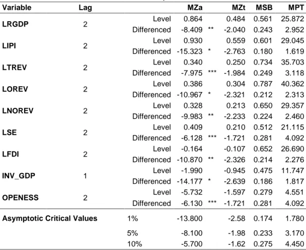
(14) Isiaka Akande Raifu and Abiodun Najeem Raheem / European Journal of Government and Economics 7(1), 60-84.. 1990 and 2000 when the non-oil revenue appears to be volatile, the economy still recorded moderate growth. However, since 2008, the growth rate of non-oil revenue and economic. 30 20 10 250. 0. 200. -10. 150. -20. 100 50. Real GDP Growth Rate (%). Non-Oil Revenue Growth Rate (%). growth seem to be synchronised, that is, to follow the same pattern.. 0 -50 82. 84. 86. 88. 90. 92. 94. 96. 98. 00. 02. 04. 06. 08. 10. 12. Real GDP Growth Rate Non-Oil Revenue Growth Rate. Figure 4. Trend of real GDP and non-oil revenues growth rates (1982-2013). From the foregoing analysis, the stylised facts about Nigerian economy in the light of the current study are summarised as follows: Before and shortly after independence in the 1960s, agriculture was the major driver of the economy. The oil sector took over as the driver of the economy in the 1970s, since when, oil revenue constitutes the bulk of government revenues. However, fluctuations of crude oil price in the international market put constraint on the government revenue generation and this affects the economy. In short, the Nigerian economy is more susceptible to oil price fluctuation in the international market, thereby putting constraint on the capacity of government to generate more revenues, to finance its planned expenditure and this ultimately affects economic progress.. 4.3. Empirical Results and Discussion 4.3.1. Unit Root Test Results. In order to avoid spurious regression analysis, it is imperative to first determine whether the variables under consideration contain unit roots or not. In other words, there is need to determine the order of integration of our variables of interest before we carry out the cointegration analysis of the relationship between government revenues and economic growth (real GDP). To achieve this, we employed Ng-Perron unit root tests. The test is carried out with intercept/constant in the regression. For a decision to be made either to reject the null hypothesis or to accept it, the computed (statistical) value of each element of the test (MZa, MZt, MSB and MPT) must be less than the asymptotic critical values. Thus, Table 2 presents the Ng-Perron unit root test results. The results show that the null hypothesis of no unit toot test cannot be rejected at the level for all the variables considered in this study. This implies that the variables are not stationary at level. They are, however, become stationary after first difference. Thus, the variables are integrated at order 1. Hence, we proceed to thr cointegration test based. 73.
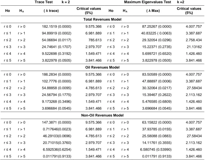
(15) Isiaka Akande Raifu and Abiodun Najeem Raheem / European Journal of Government and Economics 7(1), 60-84.. on the Johnasen cointegration test. Table 2. Ng-Perron Unit Root Test Results. Variable LRGDP LIPI LTREV LOREV LNOREV LSE LFDI INV_GDP OPENESS. Deterministic Component: Constant Lag MZa MZt Level 0.864 0.484 2 Differenced -8.409 ** -2.040 Level 0.930 0.559 2 Differenced -15.323 * -2.763 Level 0.340 0.250 2 Differenced -7.975 *** -1.984 Level 0.386 0.304 2 Differenced -10.967 * -2.321 Level 0.328 0.213 2 Differenced -9.983 ** -2.233 Level 0.409 0.210 2 Differenced -6.128 *** -1.721 Level -0.164 -0.107 2 Differenced -10.870 ** -2.326 Level -1.990 -0.945 1 Differenced -14.177 * -2.639 Level -5.732 -1.597 2 Differenced -6.130 *** -1.721. Asymptotic Critical Values. MSB 0.561 0.243 0.601 0.180 0.734 0.249 0.787 0.212 0.650 0.224 0.512 0.281 0.652 0.214 0.475 0.186 0.279 0.281. MPT 25.872 2.952 29.045 1.619 35.703 3.118 40.362 2.313 29.357 2.460 21.115 4.092 26.690 2.276 11.747 1.817 4.551 4.092. 1%. -13.800. -2.58. 0.174. 1.780. 5% 10%. -8.100 -5.700. -1.98 -1.62. 0.233 0.275. 3.170 4.450. Source: Authors’ computation using EVIEW 9 software. Note: *, **, and *** represent 1%, 5% and 10% levels of significance respectively.. 4.3.2. Cointegration Test Results. In this subsection, the question of whether cointegration exists among the variables we considered was addressed. In this case, the Johansen cointegration technique was employed. Table 3 presents the Johansen cointegration test results (with unrestricted intercept and no trend) for three models which include the total revenues model, oil revenues model and non-oil revenues model. The cointegration test was done to determine whether our variables of interest are cointegrated or not, that is, to test whether the long-run relationship holds. Since the cointegration tests are sensitive to lag selection criteria, the maximum lag length selected is two for the three models. From Table 3, it can be observed that both the total revenues model and oil revenues model have three cointegrating equations while the non-oil revenues model has only two cointegration equations. The overall results, therefore, show that our variables of. 74.
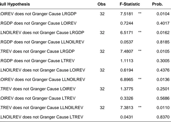
(16) Isiaka Akande Raifu and Abiodun Najeem Raheem / European Journal of Government and Economics 7(1), 60-84.. interest are cointegrated at the 5% level of significance. This implies that the long-run and shortrun models can be estimated using the ARDL cointegrating short-run and long-run method.. Table 3. Johansen Cointegration Test Results. Trace Test Ho. HA. k=2. ( λ trace). Maximum Eigenvalues Test Critical values (5%). Ho. ( λ Max). HA. k =2 Critical values (5%). Total Revenues Model r≤0. r>0. 182.1519 (0.0000). 9.575.366. r≤0. r>0. 87.25267 (0.0000). 4.007.757. r≤1. r>1. 94.89919 (0.0002). 6.981.889. r≤1. r>1. 40.83225 ( 0.0063). 3.387.687. r≤2. r>2. 54.06694 (0.0117). 785.613. r≤2. r>2. 29.32054 (0.0296). 2.758.434. r≤3. r>3. 24.74641 (0.1707). 2.979.707. r≤3. r>3. 15.22371 (0.2735). 21.13162. r≤4. r>4. 9.522698 (0.3192). 1.549.471. r≤4. r>4. 5.699721 (0.6520). 1.426.460. r≤5. r>5. 3.822978 (0.0505). 3.841.466. r≤5. r>5. 3.822978 (0.0505). 3.841.466. Oil Revenues Model r≤0. r>0. 186.2834 (0.0000). 9.575.366. r≤0. r>0. 83.50589 (0.0000). 4.007.757. r≤1. r>1. 102.7776 (0.0000). 6.981.889. r≤1. r>1. 47.88897 (0.0006). 3.387.687. r≤2. r>2. 54.88858 (0.0095). 4.785.613. r≤2. r>2. 30.32064 (0.0217). 27.58434. r≤3. r>3. 24.56794 (0.1775). 2.979.707. r≤3. r>3. 15.39467 (0.2622). 2.113.162. r≤4. r>4. 9.173268 (0.3496). 1.549.471. r≤4. r>4. 5.476585 (0.6809). 1.426.460. r≤5. r>5. 3.696684 (0.0545). 3.841.466. r≤5. r>5. 3.696684 (0.0545). 3.841.466. Non-Oil Revenues Model r≤0. r>0. 147.3871 (0.0000). 9.575.366. r≤0. r>0. 63.15822 (0.0000). 4.007.757. r≤1. r>1. 0.717646(0.0023). 6.981.889. r≤1. r>1. 37.93785 (0.0155). 3.387.687. r≤2. r>2. 46.29103(0.0696). 4.785.613. r≤2. r>2. 25.58088 (0.0883). 27.58434. r≤3. r>3. 20.71015(0.3760). 2.979.707. r≤3. r>3. 14.11761 (0.3555). 2.113.162. r≤4. r>4. 6.592536(0.6254). 1.549.471. r≤4. r>4. 6.580745 (0.53990). 1.426.460. r≤5. r>5. 0.011791(0.9133). 3.841.466. r≤5. r>5. 0.011791 (0.9133). 3.841.466. Source: Authors’ computation using EVIEWS 9 software. Note: Probability values that signify the level of significance are put in parenthesis. Also, r represents number of cointegrating vectors and k represents the number of lags in the unrestricted VAR model.. 4.3.3 Granger-Causality Test. In this subsection, we carried out a Granger-causality test to further establish the existence of relationship between government revenues and economic growth in Nigeria. In its original form, the Granger-causality test is designed to determine whether one variable can be used to forecast another variable and it is predicated on the null hypothesis of no Granger-causality between two variables. The null hypothesis will be rejected if the computed F-statistical value is greater than the critical F-statistical value. In this study, we make use of probability values obtained from the EVIEWS output to determine whether our variables of interest Granger-cause each other. The results of the Granger-causality test are presented in Table 4. The results show. 75.
(17) Isiaka Akande Raifu and Abiodun Najeem Raheem / European Journal of Government and Economics 7(1), 60-84.. that there exists a unidirectional causality between oil revenues, non-oil revenues and total revenues with the direction of causality running from oil revenue, non-oil revenue and total revenue to economic growth. In other words, oil revenue, non-oil revenue and total revenue Granger-cause economic growth in Nigeria.. Table 4. Granger-Causality Test Results Null Hypothesis. Obs. LOIREV does not Granger Cause LRGDP. 32. LRGDP does not Granger Cause LOIREV. F-Statistic 7.5181. **. 0.7244. LLNOILREV does not Granger Cause LRGDP. 32. LRGDP does not Granger Cause LLNOILREV. 6.5171. 32. LRGDP does not Granger Cause LTREV LLNOILREV does not Granger Cause LOIREV. 32. LOIREV does not Granger Cause LLNOILREV. 7.4807. **. 32. LOIREV does not Granger Cause LTREV LTREV does not Granger Cause LLNOILREV. 32. LLNOILREV does not Granger Cause LTREV. 0.0162 0.8185. **. 0.0105. 1.1113. 0.3005. 0.6194. 0.4376. 6.8965. LTREV does not Granger Cause LOIREV. 0.0104 0.4017. 0.0537. LTREV does not Granger Cause LRGDP. Prob.. **. 0.0136. 1.3775. 0.2501. 0.3326. 0.5686. 7.3813 0.0431. **. 0.0110 0.8370. Source: Authors’ computation using EVIEWS 9 software. Note: *. ** and *** denote 1%, 5% and 10% level of significance respectively.. 4.3.4. ARDL Coefficients for Long-run Form Results. Having discovered that the variables are cointegrated, the next agendum is to proceed to the estimation of a short-run dynamic and long-run estimation using the ARDL method of estimation. Table 5 presents the long-run form results for all three models. Beginning from the total revenues model, it can be observed that real GDP and total government revenues are positively and significantly related. Specifically, a 1% increase in government total revenues leads to 0.12% increase in economic growth, holding other independent variables constant (henceforth the assumption of other independent variables held constant is applicable to all). 10 Similarly, oil revenue and non-oil revenue and economic growth have a positive and significant relationship. For example, a 1% increase in oil and non-oil revenues will lead to 0.118% and 0.092% respectively. These results show that government revenues, particularly those realised from sales of crude oil, are crucial to economic growth in Nigeria. Therefore, an increase in 10. This is done to avoid repetition.. 76.
(18) Isiaka Akande Raifu and Abiodun Najeem Raheem / European Journal of Government and Economics 7(1), 60-84.. government revenues leads to an increase in economic growth. The results are akin to empirical findings by Hamdi and Sbia (2013), Ahmad and Masan (2015), Jone et al. (2015) and Ude and Agodi (2014). Specifically, Hamdi and Sbia (2013) found that oil revenue is the main source for economic growth through the channel of financing government spending. Similarly, Jone et al. (2015) concluded that there is long-run relationship between the real GDP, government expenditure and the government revenues. On the relationship between non-oil revenue and economic growth in Nigeria, Ude and Agodi (2014) noted that non-oil revenues such as agricultural revenue and manufacturing revenue have both a short-run dynamic and long-run relationship with economic growth. It must also be stated that the results could suggest indirectly that a reduction in government revenues will result in an economic growth downturn. This implies that government needs to take the issue of management of its revenues seriously and channel its realised revenues to productive projects that will not only lead to growth that is level, sustained and inclusive. This becomes important considering the source from which the largest chunk of revenues is coming. Any internal or external disturbances to the source of revenues will be detrimental for the economy and by extension increase poverty. In addition, human capital, proxied by secondary school enrolment, is also important to economic growth as well as investment (gross fixed capital formation). The two variables (human capital and investment) have positive and significant effects on economic growth. Spefically, if human capital and investment increase by 1% in all three models, economic growth will increase by 0.527%, 0.541% , 0.815 and 0.270%, 0.275% and 0.196% respectively. This result is not surprising as the literature is replete with empirical evidence of impact of human capital development and investment on economic growth both in developed and developing countries (see Barro, 1991; Barro and Lee, 2010; Cohen and Soto, 2007; Hanusheck and Woessmann, 2009). Moreover, it is found that trade openness, a measure of how a country is opened to the rest of the world in terms of trade both in goods and services as well as capital transactions) exhibits a negative relationship with economic growth. Thus, an increase in trade openness by 1% will dampen economic growth in all three models by 0.005%, 0.003% and 0.002% respectively. This finding may not be unconnected to the overdependence of the country on imports of all sorts of goods from foreign countries which, over the year, have had negative impacts on the manufacturing sector. However, foreign direct investment (FDI), though it has a positive relationship with economic growth, is not statistically significant. 11. 4.3.5. ARDL Cointegration for Short-run Model Results. In this subsection, we estimate error the correction mechanism using the ADRL method to examine the short-run relationship among the variables. The results are presented in Table 6. We can observe that the coefficients of ECT follow a priori expectation. Specifically, the coefficients are not only negative but also statistically significant at the 1% level of significance. This shows that there is a short-run dynamic adjustment towards the long-run equilibrium. The 11. The coefficient of each variable can also be explained in terms of elasticity. 77.
(19) Isiaka Akande Raifu and Abiodun Najeem Raheem / European Journal of Government and Economics 7(1), 60-84.. magnitudes of these coefficients are quite higher which depict a quicker return to the long-run equilibrium in case there is disequilibrium in the system. To be specific, the error correction term coefficients in all the three models are -0.761, -0.731 and -0.645 respectively. This shows that 76.11%, 73.13% and 64.45% errors are corrected for respectively and that it will take less than one-half years for the economics to converge to the long-run equilibrium. Table 5. Long-run Model Results. Dependent Variable: Real Gross Domestic Product (RGDP) Total Revenues. Oil Revenues. Non-Oil Revenues. Constant. 20.4488 (0.0000). 20.3351 (0.0000). 21.2272 (0.0000). LTREV. 0.1197 (0.0000). Variable. 0.1182 (0.0000). LOREV. 0.0915 (0.0000). LNOREV LSE. 0.5272 (0.0019). 0.5414 (0.0019). 0.8154 (0.0006). OPEN. -0.0052 (0.0046). -0.0027 (0.0058). -0.0018 (0.2891). LFDI. 0.0201 (0.4075). 0.0184 (0.4621). 0.0471 (0.1964). INV_GDP. 0.2702 (0.0000). 0.2752 (0.0000). 0.1957 (0.0047). Source. Authors’ computation using EVIEWS 9 software. Note. Probability values that signify the level of significance are put in parentheses.. As in the case of the long-run estimated model, total revenues and oil revenue are positively and significantly related to economic growth. However, the positive impact of elasticity coefficients of the long-run model is higher than that of the short-run model. This implies that over time government-realised revenue from the sales of crude oil, per adventure due its investment in the critical sectors of the economy, give rise to economic growth in the long-run. It is, however, observed that non-oil revenue though still having a positive relationship with economic growth is not statistically significant in the short-run. This is understandable considering the meagre amount of money being realised from those sectors of the economy. It is found that in the short-run human capital and investment still maintain positive and significant relationships with economic growth, though, at attenuated rates when compared with their effects on economic growth in the long-run model. Trade openness, in total revenues and oil revenue models, still exhibits a negative effect on economic growth at the 10% level of significance, however its lag in one period has a positive effect on economic growth at the 1% level of significance. This shows that the initial opening of the economy to the rest of the world may be profitable though dangerous over time. Thus, government and its agencies have to be wary with economic opening. Finally, foreign direct investment still does not have statistically significance in the short-run.. 78.
(20) Isiaka Akande Raifu and Abiodun Najeem Raheem / European Journal of Government and Economics 7(1), 60-84.. Table 6. Autoregressive Distribution Lag (ADRL) Cointegrating Model Results. Dependent Variable: Real Gross Domestic Product (RGDP). Variable. Total Revenues. D(LRGDP(-1)). 0.4138 (0.0094). D(LTREV). 0.0911 (0.0001). D(LOIREV). Oil Revenues 0.3997 (0.0106). 0.0350 (0.2542) -0.0485 (0.1030). D(LNOLREV(-1)) 0.4012 (0.0025). 0.3959 (0.0026). 0.5340 (0.0021) -0.3033 (0.0159). D(LSE(-1)) D(OPENESS) D(OPENESS(1)) D(LFDI). 0.4073 (0.0244). 0.0864 (0.0000). D(LNOREV) D(LSE). Non-Oil Revenues. -0.0018 (0.0788). -0.0017 (0.0829). -0.0012 (0.3118). 0.0024 (0.0096). 0.0024 (0.0084). 0.0153 (0.4130). 0.0135 (0.4673). 0.0304 (0.1973). D(IN_GDP). 0.2056 (0.0006). 0.2013 (0.0005). 0.1261 (0.0326). CointEq(-1). -0.7611 (0.0000). -0.7313 (0.0000). -0.6445 (0.0003). Source: Author’s computation using EVIEWS 9 software. Note: Probability values that signify the level of significance in parentheses.. 4.3.6. Diagnostic Test Analysis. Table 7 presents the results of diagnostic tests for the ARDL model estimated above. The tests were carried out because the validity of ARDL results rests on the satisfaction of the assumptions of Classical OLS such as normality, linearity, no serial correlation and homoscedasticity. Each of these tests has its null hypothesis against which the alternative hypothesis is tested. For example, the null hypothesis under the linearity assumption states that the model is linear in parameter while the null hypothesis of normality test is that the model is normally distributed with zero mean and constant variance. In the same vein, LM heteroscedasticity and serial correlation tests rest on the null hypotheses of homoscedasticity (equal variance) and no serial correlation respectively. The decision is made based on the nonrejection of the null hypothesis. According to the Table 7, the results show that all the models pass the tests conducted because the null hypothesis for each test cannot be rejected. This implies that the models are linear in parameter, normally distributed with zero mean and constant variance, homoscedastic (have equal variance) and suffer no serial correlation. Thus, the models are reliable and can be employed for economic policy formulation, forecasting and prediction.. 79.
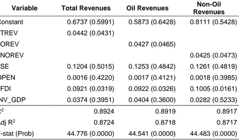
(21) Isiaka Akande Raifu and Abiodun Najeem Raheem / European Journal of Government and Economics 7(1), 60-84.. Table 7. Sensitivity/Diagnostic Tests Test. Total Revenues Model. Oil Revenues Model. Non-Oil Revenues Model. Jacque-Bera. 0.8229 (0.6627). 0.4279 (0.8074). 1.9677 (0.3739). Serial Correlation LM Test. 0.9637 (0.3994). 1.1147 (0.3486). 0.5051 (0.6122). ARCH Heteroscedasticity Test. 0.6841 (0.4152). 0.6807 (0.4163). 0.0992 (0.7551). Linearity Test. 0.0424 (0.8390). 1.20E-05 (0.9973). 0.8867 (0.3588). Source: Authors’ computation using EVIEWS 9 software Note: Probability values that signify the level of significance in parentheses.. Table 8. Robustness Check Results. Dependent Variable: Industrial Production Index. Variable. Total Revenues. Constant. 0.6737 (0.5991). LTREV. 0.0442 (0.0431). LOREV. Oil Revenues 0.5873 (0.6428). Non-Oil Revenues 0.8111 (0.5428). 0.0427 (0.0465). LNOREV. 0.0425 (0.0473). LSE. 0.1204 (0.5015). 0.1253 (0.4842). 0.1261 (0.4819). OPEN. 0.0016 (0.4220). 0.0017 (0.4121). 0.0018 (0.3985). LFDI. 0.0921 (0.0319). 0.0922 (0.0326). 0.1005 (0.0161). INV_GDP. 0.0374 (0.3951). 0.0404 (0.3600). 0.0282 (0.5233). 0.8924. 0.8919. 0.8917. R2 Adj. R2. F-stat (Prob). 0.8724. 0.8718. 0.8717. 44.776 (0.0000). 44.541 (0.0000). 44.483 (0.0000). Source: Authors’ computation using EVIEWS 9 software. Note: Probability values that signify the level of significance in parentheses.. 4.3.7. Robustness Check. In addition to assessing the impact of government revenues on economic growth proxied by real GDP and using the ARDL estimation approach, we test consistency of our findings above by using other means of economic indicator and estimation techniques. In this case, we used industrial production index (IPI) as a proxy for economic performance and OLS as a method of. 80.
(22) Isiaka Akande Raifu and Abiodun Najeem Raheem / European Journal of Government and Economics 7(1), 60-84.. estimation. 12 The results obtained from this exercise, however, are not different from that obtained using real GDP as a proxy for economic growth and the ARDL estimation method. Specifically, the results in Table 8 show that total revenues, oil revenues and non-oil revenues are positively and significantly linked with the industrial production index. It therefore implies that government revenues are indispensable to the sustenance of the Nigerian economy.. 5. Conclusion and Policy Recommendations The dynamic relationship between government revenues and economic growth has been examined in this study using the Ng-Perron unit root test technique, the Johansen cointegrated approach and the autoregressive distribution lag method. The results reveal that all revenues considered (total revenue, oil revenue and non-oil revenue) have positive effects on economic growth in both the short-run and long-run. However, it is discovered that economic growth is more responsive to oil revenues than non-oil revenues. This explains in part the rationale for economic problem whenever there is revenue shortage, occasioned most of the time by a declining oil price in the international market. Based on the results above, it is recommended that the revenues accrued to government should be frugally channelled to the critical sectors of the economy for rapid and sustainable economic growth. Specifically, government should make a concerted effort to ensure that accrued revenues are invested in the infrastructural facilities such as electricity, good roads, health care, pipe-borne water and tourism that will improve the environment and encourage economic activities. During the oil boom particularly when the oil price increases in the international market and revenues are accrued to the government, the latter should set aside money for rainy days so as to avoid the current socioeconomic crisis in the country which is caused by lack of funds. This can be achieved by keeping excess oil revenue in a special account which will be solidly backed by the law that will prevent exuberant spending. Examples of this revenue management can be adopted from other oil-producing countries such as Norway, South Arabia and the United Arab Emirates, which have been able to manage their oil revenues successfully. The saved money can be used to reflate the economy during economic recession in the future. Above all, the other sectors of the economy should be improved upon or made attractive for foreign investors so that more revenues that will serve as shock absorbers against oil price volatility can be generated.. References. Adel, Shakeeb M, (2015) 'Effects of oil and non-oil exports on the economic growth of Syria', Academic Journal of Economic Studies, Vol. 1, No. 2, pp. 69-78. 12. By definition, the industrial production index is an economic indicator used to measure the amount of output produced by different manufacturing industries in the economy while OLS is the method used in economics or statistics to estimate unknown parameters in a linear regression which could be simple regression or multiple regression. 81.
(23) Isiaka Akande Raifu and Abiodun Najeem Raheem / European Journal of Government and Economics 7(1), 60-84.. Aghion, Philippe and Howitt, Peter (1992) 'A model of growth through creative destruction' Econometrica, 60:323–351. https://doi.org/10.2307/2951599 Ahmad, Ahmad H. and Masan Salem (2015) 'Dynamic relationship between oil revenue, government spending and economic growth' International Journal of Business and Economic Development, Vol 3, No.2 Barro, Robert (991) 'Economic growth in a cross section of countries', Quarterly Journal of Economics, 106(2):407–43 Ang, James B. (2008) 'A survey of recent developments in the literature of finance and growth', Journal. of. Economic. Surveys,. 22(3):536–576.. https://doi.org/10.1111/j.1467-. 6419.2007.00542.x Ayinde, Kayode; Kuranga, John and Lukman Adewale F. (2015) 'Modelling Nigerian government expenditure, revenues and economic growth: Co-integration, error correction mechanism and combined estimators analysis approach', Asian Economic and Financial Review, 5(6):858-867. https://doi.org/10.18488/journal.aefr/2015.5.6/102.6.858.867 Baghestani, Hamid and McNown Robert (1994) 'Do revenues or expenditures respond to budgetary. disequilibria?'. Southern. Economic. Journal,. 61,. (2),. 311-322.. https://doi.org/10.2307/1059979 Barro, Robert. J. and Lee Jong-Wha (1994) 'Sources of economic growth', Carnegie-Rochester Conference Series on Public Policy 40:1-46. https://doi.org/10.1016/0167-2231(94)90002-7 Barro, Robert and Lee Jong-Wha (2010) 'A New Data Set of Educational Attainment in the World', National Bureau of Economic Research Working Paper No. 15902, Massachusetts. Boarini, Romanian; Asa Johansson and Macro Mira d'Ercode (2006) 'Alternative Measures of Wellbeing', OECD Social, Employment and Migration Working Paper 33. Buchanan, James M. and Wagner Richard W. 1978) 'Dialogues concerning fiscal religion' Journal of Monetary Economics, 4,627-636. https://doi.org/10.1016/0304-3932(78)90056-9 Cass, David (1965) 'Optimum growth in an aggregative model of capital accumulation' Review of Economic Studies 32, 233–240. https://doi.org/10.2307/2295827 Cohen, Daniel and Soto Marcelo (2007) 'Growth and human capital: Good data, good results' Journal of Economic Growth, 12:51–76. https://doi.org/10.1007/s10887-007-9011-5 Dreger, Christian and Rahmani Termur (2014) 'The Impact of Oil Revenues on the Iranian Economy and the Gulf States' Discussion Paper. Engen, Eric and Skinner Jonathan (1996) 'Taxation and economic growth', National Tax Journal, Vol.49, No. 4, pp. 617-642. https://doi.org/10.3386/w5826 Friedman, Milton (1978) 'The Limitation of Tax Limitation' Policy Review, 7-14. Grossman, Gene M. and Helpman Elhanan (1991) Innovation and Growth in the Global Economy. Cambridge, MA: MIT Press Hanushek, Eric A. and Woessmann Ludger (2009) Do Better Schools Lead to More Growth? Cognitive Skills, Economic Outcomes, and Causation NBER Working Paper No. 14633, National Bureau of Economic Research, Massachusetts Hamdi, Helmi and Sbia Rashid (2013) 'Dynamic relationships between oil revenues, government spending and economic growth in an oil-dependent economy' Journal Economic. 82.
(24) Isiaka Akande Raifu and Abiodun Najeem Raheem / European Journal of Government and Economics 7(1), 60-84.. Modelling 35, 118-125, http://dx.doi.org/10.1257/aer.20110236. Ibeh, Francisca Ujunwa (2013) 'The Impact of Oil Revenues on the Economic Growth in Nigeria' Caristas University. Jubrin, Success Musa; Blessing Success Ejura and Ifurueze M.S.K. (2014) 'Impact of petroleum profit tax on economic development of Nigeria' British Journal of Economics, Finance and Management Sciences, Vol. 5 (2), PP 60-70. Jones, Charles I. and Klenow Peter J. (2016) 'Beyond GDP? Welfare across countries and time', America Economies Review, 106(9), 2426-2457. https://doi.org/10.1257/aer.20110236 Jones, Ebieri; Ihundinihu John Uzoma. U. and Nwaiwu, J. N. (2015) 'Total revenue and economic growth in Nigeria: empirical evidence' Journal of Emerging Trends in Economics and Management Sciences (JETEMS), 6(1): 40-46 Tuffour, Joseph K (2013) 'Foreign aid, domestic revenues and economic growth in Ghana', Journal of Economics and Sustainable Development I (Online) Vol.4, No.8, www.iiste.org Kabir, Maryam (2016) 'Long-run relationship between oil revenues and economic growth in Nigeria' Archives of Business Research, 4(2), 37U47 Keynes, John Maynard (1936) (1964) The General Theory of Employment, Interest, and Money, New York: Harcourt-Brace & World, Inc. Koopmans, Tjalling C. (1965) 'On the concept of optimal economic growth: In the economic approach to development planning', Amsterdam: Elsevier. Levine, Ross and Zervos Sara (1998) 'Stock markets, banks and economic growth', American Economic Review, 88: 537–558 Levine, Ross (1997) 'Financial development and economic growth: Views and agenda', Journal of Economic Literature, XXXV:688–726 Lucas, Robert E. Jr. (1988) 'On the mechanics of economic development', Journal of Monetary Economics 22, 3–42. https://doi.org/10.1016/0304-3932(88)90168-7 Abata, Matthew A. (2014) 'The impact of tax revenues on Nigerian economy: Case of federal board of inland revenues', Journal of Policy and Development Studies, Vol. 9, No. 1 November 2014, Website: www.arabianjbmr.com/JPDS_index.php Meltzer, Allan H. and Richard Scott.F. (1981) 'A rational theory of size of government', Journal of Political Economy, 89, 914-927. https://doi.org/10.1086/261013 Mirrlees, James A (1971) 'An exploration in the theory of optimal income taxation' Review of Economic Studies 38, 175-208. https://doi.org/10.2307/2296779 Musgrave, Richard (1966) 'Principles of budget determination', in H. Cameron and W. Henderson (eds.), Public Finance Selected Reading. New York: Random House. Pg. 15-27 North, Douglass C. (1990) Institutions, Institutional Change and Economic Performance. Cambridge University Press, Cambridge. https://doi.org/10.1017/CBO9780511808678 Odularu, Gbadebo O. (2008) Crude oil and the Nigerian economic performance: oil and gas Business, http://www.ogbus.ru/eng Okafor, Regina G. (2012) 'Tax revenues generation and Nigerian economic development', European Journal of Business and Management ISSN 2222-1905 (Paper) ISSN 2222-2839. 83.
(25) Isiaka Akande Raifu and Abiodun Najeem Raheem / European Journal of Government and Economics 7(1), 60-84.. (Online) Vol. 4, No.19, 2012, www.iiste.org Peacock, Alan T. and Wiseman Jack (1979) 'Approaches to the analysis of government expenditure. growth',. Public. Finance. Review,. 7,. 3-23.. https://doi.org/10.1177/109114217900700101 Ramsey, Frank (1927) 'A contribution to the theory of taxation', Economic Journal, 37, 47-61. https://doi.org/10.2307/2222721 Ricardo, David (1820), 'Funding system' in Sraffa, P. (ed.) (1951) The Works and Correspondence of David Ricardo, Sraffa, Piero. (ed.) (1951), Cambridge University Press. Romer, Paul M. (1986) 'Increasing returns and long run growth', Journal of Political Economy, 94, 1002–1037. https://doi.org/10.1086/261420 Romer, Paul. M. (1990) 'Endogenous Technological Change' Journal of Political Economy, 98, S71–S102. https://doi.org/10.1086/261725 Singh, Ajit (1997) 'Financial liberalisation, stock markets and economic development', Economic Journal, 107: 771–782. https://doi.org/10.1111/j.1468-0297.1997.tb00042.x Slemrod, Joel (1990) 'Optimal Taxation and optimal tax systems' Journal of Economic Perspectives, 4(1), p158. https://doi.org/10.1257/jep.4.1.157 Solow, Robert M. (1956) 'A contribution to the theory of economic growth' Quarterly Journal of Economics, 70, 65–94. https://doi.org/10.2307/1884513 Ude, Damian Kalu and Agodi, Joy E. (2014) 'Investigation of the impact of non-oil revenues on economic growth in Nigeria', International Journal of Science and Research (IJSR), ISSN (Online): Volume 3 Issue 11, pp. 2571-2577 UNDP, (1990). Human Development Report. New York: Oxford University Press. Victor, Ushahemba Ijirshar (2015) 'The empirical analysis of oil revenues and industrial growth in Nigeria', African Journal of Business Management, Vol. 9(16), pp. 599- 607. https://doi.org/10.5897/AJBM2015.7801 Wagner, Adolph (1893) Grundlegung der politischen Okonomie. Leipzig: C. F. Winter.. 84.
(26)
Figure


+7


Documento similar
Therefore, it will be shown that there is a closed and necessary interdependency of digital integration and servitization in the case of agri-food sector to answer the
Carmignani(2003) found that the effect of fragmentation on growth is negative. In this study, the relation between political instability and economic growth in countries will
1) Our first conclusion is that Industry and Foreign Trade have an important role as causes that explain at a greater extent economic growth and development. In the case of
(2011) used the quantile regression methodology to explore the relationship between government size and economic growth for 24 Organisation for Economic Cooperation and
Recommendations. Several strategies have been adopted by the government to tackle the debt overhang problem of Nigeria. Examples of these are the embargo on new loans, maximum
Globalization does have a negative effect on economic growth, and although a positive effect of openness on growth is observed in the short-run, both increasing openness
Analyzing the impact of institutional factors, capital accumulation (human and physical), foreign investment, economic growth and other indicators of economic development, it
This study finds evidence that after the global financial crisis, economic growth in EU15 and Eurozone groups became more sensitive to capital flows compared to the pre-crisis period..
