Master Erasmus Mundus in
Mediterranean Forestry and Natural Resources
(MEDFOR)
Quercus suber
L. and
Quercus ilex
L. in
Spain. Updating the Provenance
Regions Maps and Calculating
Conservation Indicators for their Genetic
Resources.
Student: Leonardo Antunes Salgado Santos
Co-advisors: Ricardo Alía Miranda
José M. Garcia del Barrio
INDEX
RESUMEN ... 4
ABSTRACT ... 4
1. INTRODUCTION... 6
1.1. REGION OF PROVENANCE OF FOREST TREES... 6
1.2. THE SPECIES AND THEIR REGIONS OF PROVENANCE ... 7
1.3. CONSERVATION INDICATORS OF THE GENETIC RESOURCES ... 8
2. OBJECTIVES ... 9
3. MATERIAL AND METHODS... 9
3.1. DATA ACQUISITION AND PREPARATION ... 9
3.2. DATA ANALYSIS ... 11
3.3. MFE MAP UPDATING ... 11
4. RESULTS ... 12
4.1. QUERCUS SUBER ... 12
4.2. QUERCUS ILEX ... 17
5. DISCUSSION ... 22
6. CONCLUSIONS... 24
7. AKNOWLEDGEMENTS ... 25
RESUMEN
Las regiones de procedencia de las especies forestales, es un sistema utilizado en España y en otros países que proporciona orientación para la selección y comercialización de materiales forestales de reproducción (MFR), donde se tienen en cuenta tanto las diferencias ambientales como la variabilidad genética de las poblaciones arbóreas. Además, en el sentido de la conservación de los recursos genéticos de FRM, existen estrategias importantes para la manipulación y preservación de la capacidad de adaptación de las especies y poblaciones, como son los materiales de base (MB) y las unidades de conservación genética (UCG). El objetivo de esta investigación fue analizar y actualizar la información de los mapas de procedencia de Quercus suber L. y Quercus ilex L. en España, utilizando la información del más reciente Mapa Forestal Español (MFE50) como fuente sobre la distribución de estas especies en el país. Se investigó, además, los MB identificados, seleccionados y las UCG de ambas especies, para realizar una comparación con el MFE50 y las RP. Finalmente, el objetivo central de este trabajo se enmarcó en la incorporación de la información de origen de los rodales forestales desde el mapa RP al MFE50, mediante la creación de un nuevo atributo en la base de datos. Como resultado, se encontró que el mapa de RP fue considerablemente diferente en comparación con el MFE50, presentando un incremento en el área total de la distribución de especies en el país. Se evidenció que muchas áreas del MFE50 no están presentes en el mapa de PR y su ubicación no es exacta en municipios englobados por el Sistema de RP, por lo anterior, se recomienda incorporar y actualizar. El 35% de los MB y las UCG para las dos especies no corresponden a masas forestales en el MFE50, lo que supone la necesidad de una comprobación de campo de cara a la ubicación de estos rodales que tienen una importancia ecológica significativa. Fue posible concluir que los datos disponibles en las fuentes oficiales no son precisos a todas las escalas y deben ser revisados para proporcionar datos e información apropiados respecto a los RP, los MB y las UCG.
Palabras clave: Región de Procedencia, Mapa Forestal Español, actualización, Material de Base, Unidades de Conservación Genética.
ABSTRACT
by this system, therefore should be incorporated and updated. Many important problems were found when analysing the maps. Furthermore, when analysing the MBs and GCUs for the two species, the location of more than thirty percent of them did not correspond to any forest stands in the MFE50 map, what supposes the necessity of a field verification on face to the location of these stands that have a seminal ecological value. It was possible to conclude that the data available in the official sources are not accurate at all scales and should be revised to provide appropriate data and information regarding RPs, MBs and UCGs.
1. INTRODUCTION
1.1. Region of provenance of forest trees
Commonly, tree species that present a wide distribution range hold great levels of standing genetic diversity (Alberto et al. 2013). The Mediterranean region represents a biodiversity hotspot, where tree species are characterised by high genetic diversity within and between populations (Fady-Welterlen 2005). Many of the tree species that are present in the Mediterranean basin are genetically diverse in terms of its latitudinal and longitudinal distribution (Atkinson, Rokas, and Stone 2007). It is also to be considered that in this region the high variability respect to microclimates, geography and abiotic factors can lead to a speciation through local adaptation (Fady and Conord 2010).
When it comes to forest management practices that takes into account intra-specific variability, there is a demand for guidance on the selection of appropriated forest reproductive material and the region these materials can be deployed from their natural environment (Bower, Clair, and Erickson 2014). The genetic differences between populations characteristics, especially those related to grow, adaptation and yield, are highly important for the commercialization of reproductive forest materials (FRM). In this sense, a regionalization is established for the FRM market (European Directive 95/105) According to previous studies that analysed the adaptive capacity of tree species and populations, it was found that this characteristic is best understandable when taking into account its genetic variability and the phenotypic plasticity (Chevin, Lande, and Mace 2010; Fady et al. 2016). Although there is a lack of data on genetic variation for many native plant species, the use of a system of Regions of Provenances (or Seed Zones) is the primary guideline for seed movement and, within these geographically delimited regions, seeds of a plant species can be transferred and planted with low risk of maladaptation (Bower, Clair, and Erickson 2014).
Regions of Provenances (RP) are defined as ecologically homogeneous areas in the distribution of a species and, therefore, meant to group populations that are genetically similar and prone to be locally adapted, differing in their productivity and consequently in their impact on local economies, serving as a perfect guideline to help forest management as they serve as appropriate management units.
It is well known that species ecotypic variation exists, and the adoption of an RP system helps to secure that plant materials are adapted to the local habitat, a key aspect to consider when making a restoration or revegetation planning (Johnson et al. 2004). Furthermore, it also helps to maintain the populations’ capacity to adapt and respond to changes in the environment by preserving their integrity of natural genetic structure (Bower, Clair, and Erickson 2014). For these reasons, especially under a changing environment, the importance of forest genetic diversity is broadly recognised and should not be ignored when developing guidelines and indicators for forest management (Fady et al. 2016).
In Spain, the Regions of Provenance were defined for those species that a certification system is applicable in order to commercialize their reproductive material. The Spanish law follows the EU and OCDE scheme regarding the regulation of plant material commercialization and regions of provenance, defining it as being a zone or a group of them, delimited for a species or subspecies, that are under homogenous ecological conditions, in which seed sources or stands present similar genetic or phenotypic characteristics, taking into account limits for altitude when appropriate (RD289/2003 Art. 2.f.).
specie is present . On the other hand, the defined as “divisive method” was based on the division of the complete territory in a limited number of regions (57 regions of provenances) ecologically uniform. This regionalisation has been applied to 39 species or genera, and the delineation were adjusted to the administrative limits (Regiones de procedencia n.d.).
1.2. The species and their Regions of Provenance
Quercus suber L. cork oak as common name (“Alcornoque” in Spanish), is a widely
distributed tree species in the occidental Mediterranean region. In Spain, its distribution is predominant in the southwest of the country and it ranges from Cádiz to Salamanca and, to a lesser extent, in the province of Girona, in the northeast of the country (Heredia and Gil 2006). According to the same authors, the species only started to gain more commercial value and attention in the XX century, when it started to be replanted after centuries of overexploitation for firewood and charcoal production. It is currently most cultivated for its thick and characteristic bark that can be extracted for the production of cork used as raw material for many industrial purposes. In the Iberian Peninsula, more than 90% of cork stands are located in private lands, making it difficult to create and to develop strategies and plans to improve its conservation status, as it depends on the forest owner’s goodwill to allow the progress of the forest (Martín Albertos, Díaz-Fernández, and de Miguel 1998).
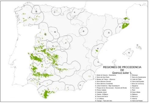
The delineation of the Regions of Provenances for cork oak in Spain consist on nine regions of wide use and seventeen Provenances of Restricted Area (Diaz Fernández et al, 1995, Martín et al, 1998, Alia et al, 2009), taking into account the ecological variation and geographical differentiation (Figure 1). The Provenances of Restricted Area are represented by letters and were created for the small forest that are present outside the main area of distribution of the species. Moreover, these regions correspond to the small regions with low economic interest for the commercial seed production but with a high ecological value
By using a variety of molecular markers, it was possible to identify groups with different genetic structures in the Iberian Peninsula. The utilization of molecular markers allows the reconstruction of the evolutionary history of the species, through the identification of demographic and historical processes of the different populations. In general terms, the neutral diversity markers are intended to provide the differences between central populations (southwest and central “dehesas” of the Iberian Peninsula) and marginal populations (cork oak stands of the east of the peninsula) (Heredia and Gil 2006).
Quercus ilex L., holm oak or holly oak as common name (“encina” in Spanish), is
the Mediterranean species that have been mostly used since the Ancient World mainly for firewood charcoal and animal feeding. Its importance has been higher for the population than cork oak, and in this sense has been favored. The consequence is the historical fragmentation and reduction of the area occupied by the cork oak (Heredia and Gil 2006). Holm oak distribution area extends to all the countries in the Mediterranean Basin and in Spain it appears in all the provinces, except the Canary Islands. It is considered the most characteristic species of the Mediterranean forests due to its wide distribution range in many different lithologic and climatic environments. This implies that it can appear as a dominant or secondary species in the majority of the peninsular territory, except in extremely dry environments with low soil fertility (Ramírez-Valiente et al. 2018). The climatic conditions and its uses have determined the characteristics of the forest of this species. In the littoral it presents in dense forest stands and inland it appears as open forests, frequently in the form of savannah-type ecosystem, known as “dehesas” in Spanish. (Alía et al. 2009).
For the delineation of the Regions of Provenances for holm oak it has been considered the climatic similarity and the geographic contiguity that can be seen in Figure 2. There are seventeen regions of wide use and eleven Provenances of Restricted Area for this species (Jiménez et al, 1996, Martín et al, 1998, Alía et al. 2009).
Figure 2: Regions of Provenance of Quercus ilex L. in Spain (Alía et al. 2009).
1.3. Conservation Indicators of the Genetic Resources
corresponding to the different admission, selection and characterization forms, and the location maps of the different units of the Catalogue are found in paper files and in the Silvadat database, developed for the management of the Catalogue (REGISTRO Y CATÁLOGO NACIONAL DE MATERIALES DE BASE n.d.).
The creation of a National Registry of Genetic Conservation Units is included in the Spanish Strategy for the Conservation and Sustainable Use of Forest Genetic Resources (MIMAM, 2006) as basic elements of in-situ and ex-situ conservation strategies. In general, the selection criteria for the Genetic Conservation Units (GCU) follows certain basic principles such as: to cover the entire area of distribution of the species targeted by the network, to ensure the natural origin of the populations subject to conservation, to restrict the management regarding the possibility of using reproductive materials not coming from the population, to give preference to the selection of units in the State lands to ensure the viability of conservation, and if possible, include a mention of the unit in the forest management plan (García del Barrio et al, 2018). The National Network of in situ conservation must cover all the spatial genetic variation of the species, as well as the most frequent alleles of each population. Therefore, it is necessary to consider the sampling of populations for each species and the size of the sample within each population. In the first case, the regions of origin of the species must be the starting point for the choice of the desired number (goal) of populations to be conserved. This number must be agreed upon by the National Committee for the Improvement and Conservation of Genetic Resources at the proposal of the National Plan for the Conservation of Genetic Resources. As a basic criterion, it is proposed to take as a reference the number of RPs of the species and prioritize the identification of genetic conservation units that include several species. Finally, it is proposed to act under the concept of MBPS to build this network (INIA 2009).
2. OBJECTIVES
The aim of this study is, through the analysis and comparison of the current maps of the regions of provenances and the latest update Spanish Forest Map (MFE) provided by the Ministry of Agriculture, Fisheries and Food (MAPAMA), to analyse the changes that the current RP’s map of Spain might have suffered and to provide a new and updated Spanish Forest Map (MFE50), with information on the origins of stands and the RP for two different tree species: Quercus ilex and Quercus suber. Furthermore, to calculate for the given species indicators for the development of programmes of conservation and use of the forest genetic resources.
Our specific objectives are:
1) Compare the forest stands in the two maps (Regions of Provenance and Spanish Forest Map) and test their equivalences
2) Assign to the maps a field corresponding to the origin of the stands that will be associated to the new updates of the Spanish Forest Map and the Forest Inventory. 3) Analyse the number of Basic Materials and Conservation Units for the two species in each one of their Regions of Provenances and confirm their location in a given forest stand in the MFE50.
3. MATERIAL AND METHODS
3.1. Data acquisition and preparation
two layers from the RP’s map has been used; one that contains the information of the limits of the several RPs for each species (RP_diss) (see ANNEX 1 and ANNEX 2), which matches with the limits of the municipalities, and a second one that is composed by polygons that corresponds to the forest stands in which the presence of the species is dominant (RP_aut) (ANNEXES 3 and 4). After the collection of the maps and selection of the layers, an operation to change the coordinate reference system (CRS) was needed in order to set all the maps in the same and current used CRS in the territory of Spain, which is EPSG:25830 - ETRS89 / UTM zone 30N.The original CRS of these maps was ED50, used at the time these maps were prepared, and if not changed before it can cause a displacement of the polygons and errors in the analysis. Afterwards, by unifying these two layers, we were able to generate the maps of the limits of Regions of Provenances with information on the forest area and its distribution in which Q. suber and Q. ilex are present. The second step of this work consisted first on the collection of the most updated Spanish Forest Map (MFE50) produced in 2015 and provided by the Ministry of Agriculture, Fisheries and Food. This map contains information on the ecology and structure of the thousands of forests stands around Spain. Regarding the tree forest species, up to three different species are contemplated, each one with its state of development. In order to extract the material that corresponded to the two tree species considered in this work from the MFE50, it was used the information represented on the table of attributes in the field SPX to infer about the presence of each species in each area. These fields correspond to the presence of a maximum of three species (SP1, SP2 and SP3) in which their presence is indicated by the code of the species in one of their fields. The specie we are going to work with are represented by the code “45” for Q. ilex
and “46” for Q. suber. This step enabled us to produce two different maps (ANNEXES 5 and 6), each one of them corresponding to the most updated forest map for each one of the species.
In order to compare the changes in the forest area, its new distribution range and update the maps, we unified the maps produced in the first step - the unification of the current maps of the limits of the region of provenances and its forest distribution, provided by CIFOR-INIA – with the maps produced in the second step – the maps extracted from the most updated Spanish Forest Map for each species.
3.2. Data analysis
The analysis was conducted by exporting the final table of attributes of the final maps to the software R, where we calculated the current area, locations and statistics of the maps as well as the changes in area. With R we also created a new table of attributes with new fields that was later incorporated to the MFE and can be used in the upcoming National Forest Inventories. The scrips used in order to run the analysis can be seen in ANNEX 9 AND ANNEX 10
We firstly calculated the total area of the original maps (MFE50 and RP_aut) as well as the area of the forest area in each of the regions of provenances. This was made by grouping the polygons of the MFE50 that overlapped with the RP_diss map in the same region of provenance and summing up their areas. Some of these polygons felt outside a region of provenance, which made us create a category “NO”, that corresponds to “no region of provenance assigned”, making it possible to infer about the area of the MFE50 that is currently outside a RP.
Afterwards, by comparing the two maps, we firstly identified the vectors of the MFE50 that were not overlapping with the current species distribution of the region of provenance’s map (RP_aut). As a result, we could obtain two classes of polygons – noRP and RP – which corresponds to polygons with no overlapping and polygons with overlapping respectively. Similarly, by analysing the overlapping and the previous and current areas of the vectors we identified the polygons which had its area reduced (RP_aut
(red)) and the ones that completed disappeared (RP_aut(des)) after the union operation.
Thus, with the identification of these vectors it was possible to calculate the total area of the RP_aut that have been lost or gained in comparison with to the most updated MFE50 for each species in each region of provenance.
Furthermore, in order to investigate about the area of dominance of the species we identified the polygons in which the species were dominant in the final combined map. The area where the species is dominant was assigned by inspecting the field “FIRST_DOMI” in the RP_aut map, which the code “D” represents that the species is dominant, and the field “SP1” in the MFE map, which the code “46” represented the presence of the species as the most important in the area.
As a result, we could calculate the total area, the number of polygons and area of the initial and final maps and the different categories of polygons created (MFE(noRP),
RP_aut (red) and RP_aut(des)) and compare this statistics with the to the ones where the
species is dominant in the two original maps.
In addition, it was inspected the number of polygons that disappeared and reduced (RP_aut (red) and RP_aut(des)) considering the cartographic source from where the
information was acquired and also the dominance of the species, in order to evaluate if there was any relationship between mismatching and cartographic source and dominance. Finally, by importing the table of attributes from the unions of the final map with BMs and GCU to R, we were able to calculate the number of Genetic Conservation Units and Basic Materials in each of the regions of provenances as well as the ones that did not match with any forest stand of the MFE50. The scrip to this last step can be found in ANNEX 3.
3.3. MFE map updating
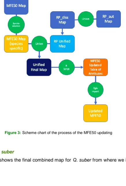
As a result of the combination of the maps of the RP and the MFE, it was generated a final map with a larger number of polygons as this operation split the polygons where they do not perfectly overlap but maintain the information of both maps in overlapping areas. This step aimed to re-extract and re-unify the polygons of the MFE from the unified map although maintaining the information regarding the origin of the species that is present in the RP map. This step was done simultaneously with the other data analysis and the details of this operation can be found in the script present in ANNEX 1 and 2 in the “Fase 3: Actualización de Mapas”. After the elaboration of the new table of attributes using R and the corresponding script, the last step was to incorporate this new table to the MFE map using Qgis. The new table of attributes that was incorporated to the MFE50 contained three fields: “id”, “area” and “origen”. The “id” of the new table created corresponded to the field “idFF2015” of the MFE50 original map table of attributes and using a join operation we could unify this two tables and inspect errors with the “area” field. A scheme chart showing the steps of the MFE50 updating is showed in Figure 3.
Figure 3: Scheme chart of the process of the MFE50 updating
4. RESULTS
4.1. Quercus suber
Figure 4: Unified final map for Q. suber.
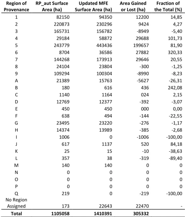
The analysis of the forested area by regions of provenances for Q. suber shows how the forested area of this species is distributed in each of them (Figure 5). The forested area of cork oak was taken from the most updated MFE and it is important to point out that restricted area regions “I”, “N”, “O” and “P”, corresponding respectively to Sierra de Carrascoy, Mallorca, Menorca and Almeria, do not have correspondence in the MFE that could justify the maintenance of the provenance regions early delimited. This may be due to the reduced extension of Q. suber patches that could have not been detected at MFE scale. This is a seminal evidence that highlights the need to periodically contrast the different forest cartographic sources available. On the other hand, in terms of its original forest area and total area of the region, Sierra Morena Ocidental (RP 5), and Sierra de San Pedro, represented by (RP 2), are the ones with the largest forested area, both of them together representing almost 40% of the total area inhabited by the species.
Figure 5: Total area forested with Q. suber by Provenance Region based on MFE data
forest area was null and they did not have any increment in the forest area after the unification with the most updated MFE, meaning these regions still do not present forest areas in which Q. suber appears as one of the three main species. Furthermore, regions of Sierra de Carrascoy and Sierra de Prades, represented by the letters “I” and “Q” respectively, do not present in the MFE any forest area where the species was present, meaning although they presented forests in the RP’s map, the most updated MFE do not show any forest area in neither of these regions. Another region that had the cork oak woodland drastically changed when comparing the two maps is the region of Pinet, represented by “L”, decreasing its area by almost 90% from the RP map to the MFE50 map. In opposite, regions of Litoral Onubense – Bajo Guadalquivir and Cuenca de Navia, represented respectively by (RP6) and “B”, showed the most increment in forest area, increasing their areas by 3,2 and 2,4 times when compared with their area in the RP map. Finally, there are some Q. suber forest area that have not been assigned yet to any provenance region, most of them detected in the latest update of the MFE.
Table 1: Total reduced or gained area after the unifications of the regions of provenances with the most updated MFE for Q. suber.
Region of
Provenance RP_aut Surface Area (ha) Surface Area (ha) Updated MFE Area Gained or Lost (ha) the Total (%) Fraction of
1 82150 94350 12200 14,85
2 220873 230296 9424 4,27
3 165731 156782 -8949 -5,40
4 29184 58872 29688 101,73
5 243779 443436 199657 81,90
6 8704 36586 27882 320,33
7 144268 173913 29646 20,55
8 24104 23804 -300 -1,25
9 109294 100304 -8990 -8,23
A 21389 15763 -5627 -26,31
B 180 616 436 242,08
C 1140 1164 024 2,15
D 12769 12377 -392 -3,07
E 450 450 000 0,00
F 638 494 -144 -22,55
G 23495 23220 -276 -1,17
H 14374 13989 -385 -2,68
I 1006 0 -1006 -100,00
J 617 1137 520 84,18
K 25 15 -10 -38,63
L 357 38 -319 -89,40
M 140 140 0 0
N 0 0 0 0
O 0 0 0 0
P 0 0 0 0
Q 219 0 -219 -100,00
No Region
Assigned 173 22643 22470 -
The total area and the area where the species is dominant in the initial MFE50 (MFE(i)) and on the updated region of provenance’s map are the same (Table 2). This result was expected, and it shows that there were almost no errors when running the data analysis as the updated map should be the same as the most updated MFE. When unifying the different maps, polygons tend to split where vectors overlap and, as a result, it produces an updated map with a significant higher number of polygons when compared to the initial maps. The number of polygons that felt outside any region of provenance (noRP) and the area their represent are relatively low compared to the total number of polygons and total area of the updated region of provenance map, representing 0,73% and 1,19 % of the totals respectively. The disappeared number of polygons are also relatively low, 1,64% of the total, and their respective area accounts for 1,32% of the original area from the updated map. The polygons that have been reduced represent a more significant amount of the total, being them 10,90% of the total number of polygons and 18,28% of the total area. The area where the species is dominant decreased in about 9 percent when comparing the updated map and the original RP map. Its respective area that felt outside any RP was 19,19 percent of the total NoRP area, and its area inside the disappeared and reduced polygons were proportional to its total area, being 38,82 and 30,64% of the total forested area of Q. suber.
Table 2: Total number of polygons, total surface area and surface area where the species is dominant in the initial maps, the updated maps and the three categories of areas created for
Q. suber.
Maps /
Categories polygons N˚ of Fraction of Total (%) Total Surface Area (ha) Fraction of Total (%) Dominance (ha) Surface of Fraction of Total (%)
MFE(i) 26741 1410391 536373 38,03
RP_aut(i) 8337 1093695 515188 47,11
MFE(upd) 48723 1410391 536373 38,03
MFE(noRP) 357 0,73 16826 1,19 3228 19,19
RP_aut(des) 799 1,64 18578 1,32 7213 38,82
RP_aut(red) 5311 10,90 257809 18,28 78998 30,64
(i) = initial map – before union, (upd) = updated map – after union, (noRP) = forest surface outside the RP_diss map, (des) = disappeared area, (red) = reduced area
Table 3: Total number of polygons according to each cartographic source and dominance of
Q. suber and its corresponding number of disappeared and reduced polygons.
Cartographic Source
/ Dominance N˚ of Polygons RP(des) (%) RP(red)
Fraction of Total (%)
AND25 11171 514 4,60 2423 21,7
IFN 121 18 14,88 24 19,8
MFE50 20868 240 1,15 2810 13,5
MFRT 374 26 6,95 54 14,4
Others 1 1 100,00 0 0,0
Dominant 18302 531 2,90 3045 16,6
Non-dominant 14233 268 1,88 2266 15,9
AND25 = Andalucía25 , IFN = Forest National Inventory, MFE50 = most updated Spanish Forest Map, MFRT = Ruiz de la Torre forest map
Table 4 presents the results of the analysis of the Conservation Indicators of the Genetic Resources for cork oak. Firstly, it is important to point out that the regions “I”, “N”, “O” and “P”, where there is no forested area detected, do not present any Identified or Selected BMs as well as conservation units for Q. suber. The number of Identified Base Materials is higher in the region RP 3 and RP 7, that correspond respectively to Montes de Toledo – Villuercas and Parque de los Alcornocales – Serranía de Ronda. These two regions collectively include a total of sixty-three out of the one-hundred-and-seventy-seven Identified BM, and five of them are outside any RP. A total of one-hundred-and-seventy-seventy-five Identified BM felt outside of any forest area, the majority of them in the region RP 3. This mismatch may be due to an imprecise location of the BM source.
Region RP 7 also presents a high number of Selected Base Materials, only behind Sierra Morena Ocidental region, represented by the RP 5. None of the regions represented by letters comprise a Selected BM. Sixteen of this selected BMs felt outside any forested area, the majority of them in the regions RP 2 and RP 5.
Table 4: Number of Base Materials and Genetic Conservation Units according to each RP for Q. suber.
Region of
Provenance Identified BM N˚ of Source- Identifies BMN˚ of Source(noMFE)
-N˚ of
Selected BM N˚ of BMSelected (noMFE)
N˚ of
GCU GCUN˚ of (noMFE)
1 11 3 7 1 1 NE
2 4 2 24 5 1 NE
3 33 20 8 1 1 NE
4 7 6 2 NE 1 1
5 14 7 36 6 1 NE
6 1 1 2 1 1 1
7 30 6 33 2 1 NE
8 3 NE 3 NE 1 NE
9 12 NE 3 NE 1 NE
A 6 3 NE NE 1 1
B 1 1 NE NE NE NE
C 3 1 NE NE 1 NE
D 13 3 NE NE 1 NE
E NE NE NE NE 1 NE
F 4 4 NE NE 1 1
G 9 6 NE NE 1 NE
H 14 6 NE NE 1 NE
I NE NE NE NE NE NE
J 1 1 NE NE 1 NE
K 1 1 NE NE 1 1
L 2 2 NE NE 1 1
M 3 2 NE NE 1 1
N NE NE NE NE NE NE
O NE NE NE NE NE NE
P NE NE NE NE NE NE
Q NE NE NE NE NE NE
No Region
Assigned 5 NE NE NE 1 NE
Total 177 75 118 16 21 7
(noMFE) = located outside a MFE forest stand, NE = non-existent
4.2. Quercus ilex
Figure 6: Unified final map for Q. ilex.
The region Extremadurense RP 11 is by far the one that gained the largest amount of forest area after the unification when compared to the other regions, increasing its surface in about 285 thousand ha (Table 5). Although in net amounts it represents a vast area, when taking into consideration that this region is the largest RP and with the most forested area, this value only accounts for an increment of 8,12 % in relation to the its initial forested area. In proportional terms the RP that suffered the greatest change in area was Sierra Nevada - Filabres (RP 16), increasing its area by more than eighty-six percent of its initial forest surface, followed by the region of Sierras Béticas Valencianas (“J”), that decreased its woodlands by more than 46%. In terms of total change in forests surface in Spain, we can observe a loss of around 225 thousand ha of forests with Q. ilex, which represents a change of only 2,77% of the total area of occurrence in the country.
Table 5: Total reduced or gained area after the unifications of the regions of provenances with the most updated MFE for Q. ilex.
Region of Provenance RP_aut Surface Area (ha) Updated MFE Surface Area (ha) Area Gained or Lost (ha)
Fraction of the Total(%)
1 501292 491996 -9296 -1,85
2 273610 271801 -1809 -0,66
3 211793 225725 13932 6,58
4 493431 469090 -24341 -4,93
5 355714 343223 -12491 -3,51
6 88939 86376 -2563 -2,88
7 157812 155950 -1862 -1,18
8 194505 187123 -7382 -3,80
9 382707 381968 -739 -0,19
10 786140 681418 -104721 -13,32
11 3508540 3793569 285029 8,12
12 427219 393823 -33396 -7,82
13 93784 122084 28300 30,18
14 129098 165720 36621 28,37
15 145452 193136 47685 32,78
16 60576 112737 52161 86,11
17 60831 57871 -2960 -4,87
A 50383 52141 1758 3,49
B 5092 4684 -408 -8,01
C 20588 17792 -2796 -13,58
D 22198 22506 308 1,39
E 6777 6571 -205 -3,03
F 14330 13529 -800 -5,59
G 6720 9157 2436 36,25
H 2193 2663 470 21,44
I 29625 21923 -7701 -26,00
J 92751 49639 -43112 -46,48
K 15901 16220 319 2,01
No Region
Assigned 406 13110 12703 -
When analyzing the results for Q. ilex, for the same reason as for Q. suber, the number of polygons also increased after the unification of the maps. In this case, there was found a small difference in the total area of the initial MFE and the updated MFE, that corresponds to an error of around 0,02%. This error is directly proportional to the area covered by the original maps and the number of divisions suffered by the polygons after unifying the maps. This is caused as the values of area tend to be an approximation and the decimals of each polygon accumulates a total error that when summing their values individually resulted in this final value. When comparing the original map of the regions of provenance with the updated MFE, the area increased in around 225 thousand ha. The results of the analysis provided by Table 6 presents the results considering the total area and the total number of polygons as being the ones presented by the updated MFE. The number of polygons and the area of the MFE(i) that felt outside the area covered by the RP map was relatively low, corresponding approximately to 0,26% of the total number of polygons and 0,09% of the total area. For the number of disappeared polygons and its corresponding area, the analysis shows they were also low, differing from the values found for the number of reduced polygons and its corresponding area, that represented 10,47 and 13,21% of the total. Finally, the area where the species is dominant also increased after the unification and only a 0,01% of this area did not correspond to any area of the RP map.
Table 6: Total number of polygons, total surface area and surface area where the species is dominant in the initial maps, the updated maps and the three categories of areas created for
Q. ilex.
Maps /
Categories polygons N˚ of Fraction of total (%) Total surface area (ha) Fraction of total (%) dominance (ha) Area of Fraction of total (%)
MFE(i) 188338 8361335 5704302 68,22
RP_aut(i) 67827 8138358 5657280 69,51
MFE(upd) 303231 8363547 5704895 68,21
MFE(noRP) 498 0,16 7240 0,09 780 10,78
RP_aut(des) 5755 1,90 53656 0,64 30783 57,37
RP_aut(red) 31735 10,47 1104728 13,21 517652 46,86
(i) = initial map – before union, (upd) = updated map – after union, (noRP) = forest surface outside the RP_diss map, (des) = disappeared area, (red) = reduced area
Table 7: Total number of polygons according to each cartographic source and dominance of Q. ilex and its corresponding number of disappeared and reduced
polygons.
Cartographic Source
/ Dominance PolygonsN˚ of RP(des) (%) RP(red)
Fraction of Total (%)
AND25 54230 4076 7,52 13400 24,71
IFN 2883 35 1,21 225 7,80
MF_RIOJA 2583 45 1,74 651 25,20
MFE50 167603 1473 0,88 16890 10,08
MFRT 6674 126 1,89 569 8,53
Dominant 156812 4468 2,85 21601 13,78
Non-dominant 77162 1287 1,67 10134 13,13
AND25 = Andalucía25 , IFN = Forest National Inventory, MFE50 = most updated Spanish Forest Map, MFRT = Ruiz de la Torre forest map
Table 8: Number of Basic Materials and Genetic Conservation Units in each RP for Q. ilex Region of
Provenance Identified MB N˚ of Source- N˚ of SourceMB (noMFE) -Identified NGCU ˚ of N(noMFE) ˚ of GCU
1 31 9 2 1
2 52 7 1 1
3 80 39 1 NE
4 22 6 1 1
5 19 3 1 NE
6 2 NE 1 NE
7 62 10 1 1
8 16 3 1 1
9 12 2 1 NE
10 131 46 1 NE
11 133 37 1 NE
12 30 13 1 NE
13 19 6 1 1
14 10 2 1 NE
15 26 4 1 NE
16 8 NE 1 NE
17 17 7 NE NE
A 1 1 1 NE
B 3 2 1 1
C 7 4 1 NE
D 4 NE 1 NE
E 5 1 1 NE
F 2 1 1 1
G 1 NE 1 NE
H NE NE 1 1
I 4 1 1 NE
J 32 21 1 NE
K 1 1 NE NE
Total 730 226 27 9
(noMFE) = located outside a MFE forest stand, NE = non-existent
5. DISCUSSION
With the results of this work, it was possible to infer about many aspects related to the current system of the regions of provenances in Spain, especially for the studied species;
Q. suber and Q. ilex. By using the MFE50 as the latest data-source for the current species
in the south-west of the country, was responsible for the greater increase in forest area of this species, gaining about 285 thousand ha of forests. Additionally, both species expanded their distribution range out of their limits of the RP_diss map, meaning new forest stands of holm and cork oak are now located in municipalities that before were not part of any RP. These stands need to be incorporated in a RP based on its location and edaphoclimatic characteristics.
Another important outcome of this work was taken by the analysis of the number of polygons that disappeared or reduced and its respective area. The disappeared polygons are related to areas where the forest does not exist in the MFE50 while the diminished ones are related to polygons that did not overlap completely well. In both cases the loss of forest area was mainly caused by miss-overlapping, which can be related to cartographic errors, misidentification or mislabelling and not actually a change in forest area. When we studied these aspects in respect to the cartographic source, in both cases the polygons extracted from Andalucía autonomous community (AND25) presented a high number of disappeared as well as reduced polygons. This could also indicate an error caused by a displacement of the polygons when overlapping with the MFE50, which could mean that vectors from this source might have suffered any kind of modification when incorporated to the RP_aut map.
When analysing the surface area where the species is dominant, we can notice that
Q. suber experienced a greater change when comparing the RP_aut and MFE50 maps,
gaining almost ten percent more area of dominance in the latest map. However, the area of dominance for Q. ilex almost did not change, being 69,51% of the total area of the RP_aut map and 68,22 in the MFE50 map. This can also be explained when investigating the area where the species is dominant that is located outside any RP, which reached almost 20% of the total area outside any RP, while for Q. ilex this value was only about 10%. For both species, still considering the area where the species is dominant, the area related to the disappeared polygons tended to be slightly higher in relative terms than the area related to the reduced polygons, meaning that removed forest stands are more related to stands where the species are dominant. For Q. ilex, more than 57% of the disappeared area was forest stands where this species was dominant, which indicates a positive relationship between both aspects. Similarly, in both cases, the number of disappeared polygons where the species were dominant tended to be slightly higher when compared to the number of disappeared polygons where the species were non-dominant, indicating also a positive relationship between these two factors. Nevertheless, the number of reduced polygons did not show a significant difference between areas of dominance and non-dominance for the two species.
The Genetic Conservation Units analysis for Q. suber also showed some problems with its distribution and locations. Even though region of Cuenca de Navia (B) is the only RP without a GCU, besides the ones without forest area, many others RPs have their GCUs mismatching any forest area of the, which is the case of Sierra Morena Oriental (4), Litoral Onubense (RP 6), Galicia-El Bierzo (A), Sierra de Guadarrama (F), País Basco (K), Pinet (L) y Duero Medio (M). Coincidently some of these regions (RP 6, K and L) also had all their BMs location not in MFE forest stand and it is important to confirm and revise this information on the field to guarantee if these problems are related to a cartographic error or if the forest stand have been actually removed from the area. The results for Q. ilex also highlighted some problems related to the GCUs. Again, one RP do not have any GCU in their area, which is the case of Mallorca (RP 17), and a total of eight regions have their GCU in a location that do not coincide with the MFE50 map, which is the case of regions Cuenca Central del Duero (RP 2), Prepirineo (RP 4), Sierras de Ávila y Segovia RP˚ 7), Sur de Guadarrama (RP 8), Sierra de Cádiz-Ronda (RP 13), Asturias (B), Monegros (F), Sierras Almerienses (H). Some of these mismatch cases would be related to the accuracy of the coordinates collected from the bibliography on studies with genetic markers of this species. In any case, field work will be necessary for establishing the location and dimension of the forest stands that could be designed as GCUs.
6. CONCLUSIONS
With the main outcomes of this study it was possible to conclude that exists some unresolved questions regarding the updating of information. The analysis shows that the current data available are not satisfactory coupled. With the first part of this study we could notice that the RP_aut map and the MFE50 present some significative differences and this could be due to updating mistakes in-between forest inventories, misidentification, cartographic errors or actually a change in the species distribution area, therefore these mismatches are areas that should be revised in the field. Moreover, the system of the Regions of Provenances in Spain should also be revised, not only for the studied species relevant in this work but also for other species that had their distribution range modified in last few years. It is clear that not only forest areas disappeared from the RP map but also many new forest areas are now present in the MFE50, especially in locations that were not part of the system of RP. After the confirmation that these are new areas in which the species is present but with no RP assigned to them, they should then be incorporated in the RP map throughout an evaluation of its location and its edaphoclimatic characteristics. In the case of Q. suber, the regions “I”, “N”, “O”, “P” and “Q” should be given special attention for the fact that they do not present any forest area located in the MFE50 and an inspection has to be done to confirm this situation. The second part of this study revealed important aspects related to the Conservation Indicators of the Forest Genetic Resources. Besides the fact that some of the RPs do not present any source-identified Basic Material, many of the RPs have all BMs located in areas that do not coincide with a forest stand from the MFE50 map. This is similar when considering the Genetic Conservation Units. Furthermore, some regions do not present any GCU and also have a BM located out of a forest area, which is the case of or region Cuenca de Navia (“B”) for Q. suber and Menorca (“K”) for Q. ilex and a special attention should be given to them, as their location is known to be situated in autochthonous forest stands.
7. AKNOWLEDGEMENTS
8. REFERENCES
Alberto, Florian J. et al. 2013. “Potential for Evolutionary Responses to Climate
Change - Evidence from Tree Populations.”
Global Change Biology
19(6):
1645–61. http://www.ncbi.nlm.nih.gov/pubmed/23505261 (May 29, 2019).
Alía, R., García del Barrio, J. M., Iglesias Sauce, S., Mancha Núñez, J. A., de
Miguel y del Ángel, J., Nicolás Peragón, J. L., Pérez Martín, F.,Sánchez de
Ron, D. (2009). Regiones de procedencia de especies forestales en
España.Organismo Autónomo Parques Nacionales. Madrid
Atkinson, Rachel J., Antonis Rokas, and Graham N. Stone. 2007. “Longitudinal
Patterns in Species Richness and Genetic Diversity in European Oaks and
Oak Gallwasps.” In
Phylogeography of Southern European Refugia
,
Dordrecht: Springer Netherlands, 127–51.
http://link.springer.com/10.1007/1-4020-4904-8_4 (May 30, 2019).
Bower, Andrew D., J. Bradley St. Clair, and Vicky Erickson. 2014. “Generalized
Provisional Seed Zones for Native Plants.”
Ecological Applications
24(5):
913–19. http://doi.wiley.com/10.1890/13-0285.1 (May 29, 2019).
Chevin, Luis-Miguel, Russell Lande, and Georgina M. Mace. 2010. “Adaptation,
Plasticity, and Extinction in a Changing Environment: Towards a Predictive
Theory” ed. Joel G. Kingsolver.
PLoS Biology
8(4): e1000357.
http://dx.plos.org/10.1371/journal.pbio.1000357 (May 30, 2019).
Díaz-Fernández, PM, Jiménez, P, Catalán, G,Martín, S, GIl, L.1995. Regiones de
Procedencia de
Quercus suber
L. ICONA. Madrid.
Fady-Welterlen, Bruno. 2005. “Is There Really More Biodiversity in
Mediterranean Forest Ecosystems?”
TAXON
54(4): 905–10.
https://onlinelibrary.wiley.com/doi/abs/10.2307/25065477 (May 30, 2019).
Fady, Bruno et al. 2016. “Forests and Global Change: What Can Genetics
Contribute to the Major Forest Management and Policy Challenges of the
Twenty-First Century?”
Regional Environmental Change
16(4): 927–39.
http://link.springer.com/10.1007/s10113-015-0843-9 (May 30, 2019).
Fady, Bruno, and Cyrille Conord. 2010. “Macroecological Patterns of Species
and Genetic Diversity in Vascular Plants of the Mediterranean Basin.”
Diversity and Distributions
16(1): 53–64.
http://doi.wiley.com/10.1111/j.1472-4642.2009.00621.x (May 30, 2019).
García del Barrio, JM, Auñón, F, Martínez Fernández, J, Sánchez de Ron, D,
Alía, R. 2018. Las Unidades de Conservación de Recursos Genéticos
Forestales en el marco de la Estrategia Española para la Conservación y el
Uso Sostenible de los Recursos Genéticos Forestales Foresta 70, 66-70
Heredia, U. López de, and L. Gil. 2006. “La Diversidad En Las Especies
Forestales: Un Cambio de Escala. El Ejemplo Del Alcornoque.”
Diversity
2(2): 1–9.
INIA. 2009. “Unidades de Conservación Genética: Criterios Para La Aprobación
de Las Unidades y Su Identificación, Seguimiento y Gestión.”
http://www.inia.es/gcontrec/pub/CRITERIOS_UCRGFs_270109_123659229
8906.pdf.
Jiménez, P, Díaz-Fernández, PM, Martín, S, Gil, L. 1996. Regiones de
Procedencia de
Quercus ilex
L. ICONA. Madrid.
https://www.fs.usda.gov/treesearch/pubs/25517 (May 29, 2019).
Martín Albertos, Sonia, Pedro M. Díaz-Fernández, and Jesús de Miguel. 1998.
“Regiones de Procedencia de Las Especies Forestales Españolas. Géneros
Abies, Fagus, Pinus y Quercus.” Organismo Autónomo Parques Nacionales.
Madrid.
MIMAM. 2006.
Estrategia de Conservación y uso sostenible de los recursos
genéticos forestales
. DGB. Madrid 81 pp.
Ramírez-Valiente, José-Alberto et al. 2018. “Increased Root Investment Can
Explain the Higher Survival of Seedlings of ‘Mesic’ Quercus Suber than
‘Xeric’ Quercus Ilex in Sandy Soils during a Summer Drought.”
Tree
Physiology
39(1): 64–75.
https://academic.oup.com/treephys/advance-article/doi/10.1093/treephys/tpy084/5067533 (July 3, 2019).
“Regiones de Procedencia.”
https://www.mapa.gob.es/es/desarrollo-
rural/temas/politica-forestal/recursos-geneticos-forestales/rgf_regiones_procedencia.aspx (May 29, 2019).
“REGISTRO Y CATÁLOGO NACIONAL DE MATERIALES DE BASE.”
ANNEX 9 – R SCRIPT FOR MAP ANALYSIS AND UPDATING FOR QUERCUS SUBER
############ ACTUALIZACIÓN MAPAS REGIONES DE PROCEDENCIA SEGUN MAPA FORESTAL ESPAÑOL######
################################# Librerias ##############################################
library(foreign) #importar dbf
library(rgdal) library(sp) library(dplyr)
library(openxlsx)#requiere instalar Rtools en el ordenador
########################################################################################## #Establecer directorio
setwd("C:/")
##################### Fase 1: explorar datos cartografia inicial #########################
tablas<-list.files(pattern = ".dbf") tablas
########## Mapa de las Regiones de Procedencia
RP_diss <-read.dbf("Quercuessuber_diss.dbf") names(RP_diss)
levels(RP_diss$REGION_46)
RP_diss$REGION_46 <- factor(RP_diss$REGION_46,
levels = c( "1", "2", "3", "4", "5", "6", "7", "8", "9", "A", "B", "C", "D", "E", "F", "G", "H", "I", "J", "K", "L", "M", "N", "O", "P", "Q", "No"))
RP_diss$REGION_46[is.na(RP_diss$REGION_46)] <- "No" View(RP_diss)
########## Mapa Forestal Español Especie objetivo
MFE_Sp<-read.dbf("Species_dist_46.dbf") names(MFE_Sp)
######### Mapa Regiones de Procedencia autóctonas
RP_Sp_aut<-read.dbf("QuercussuberRP.dbf") names(RP_Sp_aut)
######## Mapa RP autóctonas con Cod_RP
RP_Sp_cod<-read.dbf("RP_Qsuber_cod.dbf") names(RP_Sp_cod)
# Ver qué regiones hay y añadir valor "no" para evitar problemas con NA no explícitos
levels(RP_Sp_cod$REGION_46)
RP_Sp_cod$REGION_46 <- factor(RP_Sp_cod$REGION_46, levels = c( "1", "2", "3", "4", "5", "6", "7", "8", "9", "A", "B", "C", "D", "E", "F", "G", "H", "I", "J", "K", "L", "M", "N", "O", "P", "Q", "No"))
View(RP_Sp_cod)
# Captura datos iniciales: núm polígonos, Superficie total, superficie sp dominante
Mapa_nombre_i <- c("MFE(i)", "RPaut(i)")
Num_pol_i<-c(nrow(data.frame(MFE_Sp)), nrow(data.frame(RP_Sp_aut))) Sup_tot_i<-c(sum(MFE_Sp$Shape_Area),sum(RP_Sp_aut$Shape_Area))
#Extraer polígonos con la sp dominante
MFE_Dom<-subset(MFE_Sp, SP1=="46")
RP_aut_Dom<- subset(RP_Sp_aut, FIRST_DOMI=="D")
Sup_Dom_i<-c(sum(MFE_Dom$Shape_Area), sum(RP_aut_Dom$Shape_Area))
############# Fase2: Importar datos Unión de mapas MFE con RP según escenarios #################
# Importo datos según escenarios en bruto definidos en GIS
MFE_RP<-read.dbf("Qsuber_MF_RP.dbf") names(MFE_RP)
View(MFE_RP)
# Renombrar variables para usar script genérico
MFE_RP <- MFE_RP %>% rename(FID_MFE ="FID_Specie", Region = "REGION_46", FID_RP = "FID_Quercu", Escenario = "SCOPE",
Dominancia = "FIRST_DOMI", FID_RPaut = "FID_Quer_1") names(MFE_RP)
####
# Ver qué regiones hay y añadir valor "no" para evitar problemas con NA no explícitos
levels(MFE_RP$Region)
MFE_RP$Region <- factor(MFE_RP$Region,
levels = c( "1", "2", "3", "4", "5", "6", "7", "8", "9", "A", "B", "C", "D", "E", "F", "G", "H", "I", "J", "K", "L", "M", "N", "O", "P", "Q", "No"))
MFE_RP$Region[is.na(MFE_RP$Region)] <- "No" View(MFE_RP)
#Lista codigo de la RP de la especie
Cod_RP<-list(unique(MFE_RP$Region)) Cod_RP
### Subset segun escenarios # MFE sin unión con RP (MFE_solo)
MFE_solo = subset(MFE_RP, Escenario == 1)
# RP sin unión con MFE (RP_solo)
RP_solo = subset(MFE_RP, Escenario ==2)
# MFE unido RP
MFE_RP_solo= subset(MFE_RP, Escenario ==3)
########## Fase 3: Actualización de mapas ################################################ # 1º Mapa MFE actualizado con RP
MFE_RP_merge = merge(MFE_solo, MFE_RP_solo, all= TRUE)
mut1<-mutate(group_by(MFE_RP_merge, FID_MFE), total_area=sum(AREA_M2))
#Extraigo polig cuya area ha aumentado
MFE_RP_act<-subset(mut1, FID_RP > -1 | total_area>AREA_M2) View(MFE_RP_act)# RP actualizado
#MFE completo con RP actualizadas
MFE_Act<-mutate(mut1, RPactual = if (FID_RP >=0 | total_area>AREA_M2) { "RP"
} else { "noRP" }) warnings() View(MFE_Act)
#Exportar a excel
write.xlsx(MFE_Act,"~/Desktop/Thesis/Results/MFE_Act_Qsuber.xlsx", asTable = FALSE)
#Paso 2
MFE_RP_act<- mutate(MFE_Act, Origen = if(Orig_num <=1.9){ "A"
} else if (RPactual == "noRP"){ "NoRP"
} else { "R" })
View(MFE_RP_act)
#Exportar a excel
write.xlsx(MFE_Act,"~/Desktop/Thesis/Results/MFE_Act_Qsuber.xlsx", asTable = FALSE)
# Versión corta
MFE_Act_exp <- data.frame(id=c(MFE_RP_act$IdFF2015),area=c(MFE_RP_act$total_area),Origen=c(MFE_RP_act$Origen)) MFE_Act_exp<- distinct(MFE_Act_exp, id, area, Origen)
View(MFE_Act_exp)
write.xlsx(MFE_Act_exp,"~/Desktop/Thesis/Results/MFE_Act_exp_Qsuber.xlsx", asTable = FALSE) summary(MFE_Act_exp$Origen)
#Error: control variación en area total MFE antes y después
E_Sup_MFE <- sum(MFE_Sp$Shape_Area) -sum(MFE_Act$AREA_M2) E_Sup_MFE
# 2º Identificacion RP poblaciones desaparecidas/disminuidas. #Unico archivo para exportar
RP_Desap<-mutate(RP_solo, RPactual = if_else (RP_solo$Shape_Area > RP_solo$AREA_M2, "RP_dism","RP_desap")) View(RP_Desap)
write.xlsx(RP_Desap,"~/Desktop/Thesis/Results/RP_Desap_Qsuber.xlsx", asTable = FALSE)
################ Analisis de resultados ####################################### ## Separo Regiones de Procedencia autóctonas y no autóctonas
# Mapa MFE Actualizado
MFE_Act
MFE_noRP <- subset (MFE_Act, RPactual == "noRP") #polígonos MFE sin RP asociada # Mapa RP desaparecidas/disminuidas
RP_dism <- subset(RP_Desap, RPactual== "RP_dism" & FID_RPaut >0) View(RP_dism)
######### Estudio de superficies #########################################
Mapa_nombre_f<- c("MFE_act", "MFE(noRP)","RP(desap)", "RP(dism)") Num_pol_f<- c(nrow(MFE_Act), nrow(MFE_noRP), nrow(RP_desap), nrow(RP_dism))
Sup_tot_f<- c(sum(MFE_Act$AREA_M2), sum(MFE_noRP$AREA_M2), sum(RP_desap$AREA_M2), sum(RP_dism$AREA_M2))
### Superficies según dominancia
RP_act_SP1 <-subset(MFE_Act, SP1==46) MFE_noRP_SP1 <-subset(MFE_noRP, SP1==46) RP_desap_SP1 <-subset(RP_desap, Dominancia == "D") RP_dism_SP1 <-subset(RP_dism, Dominancia == "D")
SUP_Dom_f <- c(sum(RP_act_SP1$AREA_M2),sum(MFE_noRP_SP1$AREA_M2), sum(RP_desap_SP1$AREA_M2),sum(RP_dism_SP1$AREA_M2))
#### Generar Data frame con resultados de superficies
Mapas<-c(Mapa_nombre_i,Mapa_nombre_f) Num_polig<-c(Num_pol_i, Num_pol_f) Sup_total<-c(Sup_tot_i, Sup_tot_f) Sup_Domin<-c(Sup_Dom_i, SUP_Dom_f) Data_analisis<-data.frame(Mapas,Num_polig, Sup_total,Sup_Domin) View(Data_analisis)
######## Estudio de poblaciones desap/dism # Segun fuente cartográfica
#Crear mapa fuentes donde solo haya FID_RPaut >-1
MFE_Act_FUENTES= subset(MFE_RP, FID_RPaut >=0) Fuentes <- data.frame(RP_des=c(summary(RP_desap$FUENTE)), RP_dis=c(summary(RP_dism$FUENTE)))
Total_Fue=c(summary(MFE_Act_FUENTES$FUENTE)) View(Fuentes)
View(Total_Fue)
# Según dominancia
Dominanc <- data.frame(RP_des=c(summary(RP_desap$Dominancia)), RP_dis=c(summary(RP_dism$Dominancia)))
Total_Dom=c(summary(MFE_RP$Dominancia)) View(Dominanc)
View(Total_Dom)
##### Exportar resultados como libro excel
wb<-createWorkbook()
addWorksheet(wb, "Superficies") writeData(wb, "Superficies", Data_analisis) addWorksheet(wb, "Fuentes")
writeData(wb, "Fuentes", Fuentes, rowNames= TRUE) addWorksheet(wb, "Dominancia")
saveWorkbook(wb, "~/Desktop/Thesis/Results/Datos_Qsuber.xlsx", overwrite = TRUE)
#####
# Superficies Por Regiones de Procedencia # MFE_Act
Reg_MFE_Act<-mutate(group_by(MFE_Act, Region), SupRP=sum(AREA_M2))
SupRP_act<-unique(data.frame(CodRP = c(Reg_MFE_Act$Region),SupMFEact=c(Reg_MFE_Act$SupRP))) View(SupRP_act)
write.xlsx(SupRP_act,"~/Desktop/Thesis/Results/SupRP_act_Qsuber.xlsx", asTable = FALSE)
#MFE(i)
MFEiRP= subset(MFE_RP, FID_MFE >=0)
Reg_MFEi<-mutate(group_by(MFEiRP, Region), SupMFEiRP=sum(AREA_M2))
SupMFEi<-unique(data.frame(CodRP = c(Reg_MFEi$Region),SupMFEi=c(Reg_MFEi$SupMFEiRP))) View(SupMFEi)
write.xlsx(SupMFEi,"~/Desktop/Thesis/Results/SupMFE(i)_Qsuber.xlsx", asTable = FALSE)
#RP(i)
Reg_RPi<-mutate(group_by(RP_diss, REGION_46), SupRPi=sum(Shape_Area))
SupRPi<-unique(data.frame(CodRP = c(Reg_RPi$REGION_46),SupRPi=c(Reg_RPi$SupRPi))) View(SupRPi)
write.xlsx(SupRPi,"~/Desktop/Thesis/Results/SupRP(i)_Qsuber.xlsx", asTable = FALSE)
#RP(i)RP
RPiRP= subset(RP_Sp_cod, FID_Autoct >=0)
Reg_RPiRP<-mutate(group_by(RPiRP, REGION_46), SupRPiRP=sum(Shape_Area))
SupRPiRP<-unique(data.frame(CodRP = c(Reg_RPiRP$REGION_46),SupRPiRP=c(Reg_RPiRP$SupRPiRP))) View(SupRPiRP)
write.xlsx(SupRPiRP,"~/Desktop/Thesis/Results/SupRP(i)RP_Qsuber.xlsx", asTable = FALSE)
#MFE_RP
Reg_MFE_RP<-mutate(group_by(MFE_RP, Region), Sup_MFE_RP=sum(AREA_M2))
SupMFE_RP<-unique(data.frame(CodRP = c(Reg_MFE_RP$Region),SupMFE_RP=c(Reg_MFE_RP$Sup_MFE_RP))) View(SupMFE_RP)
write.xlsx(SupMFE_RP,"~/Desktop/Thesis/Results/SupMFE_RP_Qsuber.xlsx", asTable = FALSE)
#RPaut_Desap
Reg_RP_Desap<-mutate(group_by(RP_desap, Region), SupRP=sum(AREA_M2))
Sup_RP_Desap<-data.frame(CodRP=c(Reg_RP_Desap$Region), SupRPDes=c(Reg_RP_Desap$SupRP)) Sup_RP_Desap<-unique(Sup_RP_Desap)
View(Sup_RP_Desap)
write.xlsx(Sup_RP_Desap,"~/Desktop/Thesis/Results/Sup_RP_Desap_Qsuber.xlsx", asTable = FALSE)
#RP_dism
Reg_RP_Dism<-mutate(group_by(RP_dism, Region), SupRP=sum(AREA_M2))
Sup_RP_Dism<-data.frame(CodRP=c(Reg_RP_Dism$Region), SupRPDis=c(Reg_RP_Dism$SupRP)) Sup_RP_Dism<-unique(Sup_RP_Dism)
View(Sup_RP_Dism)
write.xlsx(Sup_RP_Dism,"~/Desktop/Thesis/Results/Sup_RP_Dis_Qsuber.xlsx", asTable = FALSE)
###### Sup x RP
Sup_RP<- data.frame(MFE_Act =c(unique(Reg_MFE_Act$SupRP)), RP_Desap =c(unique(Reg_RP_Desap$SupRP)), RP_Dism=c(unique(Reg_RP_Dism$SupRP)))
##### Num poligonos x RP
RP_Dism=c(summary(RP_dism$Region))) View(Npol_data)
ANNEX 10 -
R SCRIPT FOR MAP ANALYSIS FOR QUERCUS ILEX############ ACTUALIZACIÓN MAPAS REGIONES DE PROCEDENCIA SEGUN MAPA FORESTAL ESPAÑOL######
################################# Librerias ##############################################
library(foreign) #importar dbf
library(rgdal) library(sp) library(dplyr)
library(openxlsx)#requiere instalar Rtools en el ordenador
########################################################################################## #Establecer directorio
setwd("C:/Users/User/Desktop")
#getwd()
##################### Fase 1: explorar datos cartografia inicial ######################### #Explorar directorio
tablas<-list.files(pattern = ".dbf") tablas
########## Mapa de las Regiones de Procedencia
RP_diss <-read.dbf("Qilex_diss.dbf") names(RP_diss)
levels(RP_diss$Region45)
RP_diss$Region45 <- factor(RP_diss$Region45,
levels = c( "1", "2", "3", "4", "5", "6", "7", "8", "9", "10", "11", "12", "13", "14", "15", "16", "17", "A", "B", "C", "D", "E", "F", "G", "H", "I", "J", "K", "No"))
RP_diss$Region45[is.na(RP_diss$Region45)] <- "No" View(RP_diss)
########## Mapa Forestal Español Especie objetivo
MFE_Sp<-read.dbf("Species_dist_45.dbf") names(MFE_Sp)
######### Mapa Regiones de Procedencia autóctonas
RP_Sp_aut<-read.dbf("QuercusilexRP.dbf") names(RP_Sp_aut)
######## Mapa RP autóctonas con Cod_RP
RP_Sp_cod<-read.dbf("RP_Qilex_cod.dbf") names(RP_Sp_cod)
# Ver qué regiones hay y añadir valor "no" para evitar problemas con NA no explícitos
levels(RP_Sp_cod$Region45)
RP_Sp_cod$Region45 <- factor(RP_Sp_cod$Region45,
levels = c( "1", "2", "3", "4", "5", "6", "7", "8", "9", "10", "11", "12", "13", "14", "15", "16", "17", "A", "B", "C", "D", "E", "F", "G", "H", "I", "J", "K", "No"))
# Captura datos iniciales: núm polígonos, Superficie total, superficie sp dominante
Mapa_nombre_i <- c("MFE(i)", "RPaut(i)")
Num_pol_i<-c(nrow(data.frame(MFE_Sp)), nrow(data.frame(RP_Sp_aut))) Sup_tot_i<-c(sum(MFE_Sp$Shape_Area),sum(RP_Sp_aut$Shape_Area))
#Extraer polígonos con la sp dominante
MFE_Dom<-subset(MFE_Sp, SP1=="45")
RP_aut_Dom<- subset(RP_Sp_aut, FIRST_DOMI=="D")
Sup_Dom_i<-c(sum(MFE_Dom$Shape_Area), sum(RP_aut_Dom$Shape_Area))
############# Fase2: Importar datos Unión de mapas MFE con RP según escenarios #################
# Importo datos según escenarios en bruto definidos en GIS
MFE_RP<-read.dbf("MFE_RP_Qilex.dbf") names(MFE_RP)
View(MFE_RP)
# Renombrar variables para usar script genérico
MFE_RP <- MFE_RP %>% rename(FID_MFE ="FID_Specie", Region = "Region45", FID_RP = "FID_Quercu", Escenario = "SCOPE",
Dominancia = "FIRST_DOMI", FID_RPaut = "FID_Quer_1") names(MFE_RP)
####
# Ver qué regiones hay y añadir valor "no" para evitar problemas con NA no explícitos
levels(MFE_RP$Region)
MFE_RP$Region <- factor(MFE_RP$Region,
levels = c( "1", "2", "3", "4", "5", "6", "7", "8", "9", "10", "11", "12", "13", "14", "15", "16", "17", "A", "B", "C", "D", "E", "F", "G", "H", "I", "J", "K", "No"))
MFE_RP$Region[is.na(MFE_RP$Region)] <- "No" View(MFE_RP)
#Lista codigo de la RP de la especie
Cod_RP<-list(unique(MFE_RP$Region)) Cod_RP
#####Generar un campo binario para hacer la union de la tabla al mapa
### Subset segun escenarios # MFE sin unión con RP (MFE_solo)
MFE_solo = subset(MFE_RP, Escenario == 1)
# RP sin unión con MFE (RP_solo)
RP_solo = subset(MFE_RP, Escenario ==2)
# MFE unido RP
MFE_RP_solo= subset(MFE_RP, Escenario ==3)
########## Fase 3: Actualización de mapas ################################################ # 1º Mapa MFE actualizado con RP
#sumo areas mismo FID_MFE
mut1<-mutate(group_by(MFE_RP_merge, FID_MFE), total_area=sum(AREA_M2))
#Extraigo polig cuya area ha aumentado
MFE_RP_act<-subset(mut1, FID_RP > -1 | total_area>AREA_M2) View(MFE_RP_act)# RP actualizado
#MFE completo con RP actualizadas
MFE_Act<-mutate(mut1, RPactual = if (FID_RP >=0 | total_area>AREA_M2) { "RP"
} else { "noRP" }) warnings() View(MFE_Act)
#Exportar a excel
write.xlsx(MFE_Act,"~/Desktop/Thesis/Results/MFE_Act_Qilex.xlsx", asTable = FALSE)
#Paso 2
MFE_RP_act<- mutate(MFE_Act, Origen = if(Orig_num <=1.9){ "A"
} else if (RPactual == "noRP"){ "NoRP"
} else { "R" })
View(MFE_RP_act)
#Exportar a excel
write.xlsx(MFE_Act,"~/Desktop/Thesis/Results/MFE_Act_ilex.xlsx", asTable = FALSE)
# Versión corta
MFE_Act_exp <- data.frame(id=c(MFE_RP_act$IdFF2015),area=c(MFE_RP_act$total_area),Origen=c(MFE_RP_act$Origen)) MFE_Act_exp<- distinct(MFE_Act_exp, id, area, Origen)
View(MFE_Act_exp)
write.xlsx(MFE_Act_exp,"~/Desktop/Thesis/Results/MFE_Act_exp_Qilex.xlsx", asTable = FALSE) summary(MFE_Act_exp$Origen)
#Error: control variación en area total MFE antes y después
E_Sup_MFE <- sum(MFE_Sp$Shape_Area) -sum(MFE_Act$AREA_M2) E_Sup_MFE
#2º Identificacion RP poblaciones desaparecidas/disminuidas. #Unico archivo para exportar
RP_Desap<-mutate(RP_solo, RPactual = if_else (RP_solo$Shape_Area > RP_solo$AREA_M2, "RP_dism","RP_desap")) View(RP_Desap)
write.xlsx(RP_Desap,"~/Desktop/Thesis/Results/RP_Desap_Qilex.xlsx", asTable = FALSE)
################ Analisis de resultados ####################################### ## Separo Regiones de Procedencia autóctonas y no autóctonas
# Mapa MFE Actualizado
MFE_Act
MFE_noRP <- subset (MFE_Act, RPactual == "noRP") #polígonos MFE sin RP asociada # Mapa RP desaparecidas/disminuidas