Phenomenology of symmetry breaking from extra dimensions

Texto completo

(1)Journal of High Energy Physics. Related content. Phenomenology of symmetry breaking from extra dimensions To cite this article: Jorge Alfaro et al JHEP01(2007)005. - Scalar dark matter in an extra dimension inspired model Roberto Lineros and Fabio Pereira dos Santos - Extended gauge symmetries and extra dimensions at the large hadron collider A Meyer - Climate change – a challenge for the arctic indigenous peoples – the Inuit response Aqqaluk Lynge. View the article online for updates and enhancements.. Recent citations - Effective field theory for magnetic compactifications Wilfried Buchmuller et al - One-loop effective potential in M_{4}×T^{2} with and without ’t Hooft flux A. Faedo et al - Flavor structure from magnetic fluxes and non-Abelian Wilson lines Hiroyuki Abe et al. This content was downloaded from IP address 146.155.157.160 on 10/05/2018 at 16:36.

(2) Published by Institute of Physics Publishing for SISSA Received: June 16, Revised: November 3, Accepted: November 25, Published: January 4,. 2006 2006 2006 2007. Phenomenology of symmetry breaking from extra dimensions. Facultad de Fı́sica, Pontificia Universidad Católica de Chile, Casilla 306, Santiago 22, Chile E-mail: jalfaro@uc.cl. Alicia Broncano Max Planck Institute for Physics, Föhringer Ring 6, 80805 Munich, Germany E-mail: broncano@mppmu.mpg.de. Maria Belen Gavela, Stefano Rigolin and Matteo Salvatori Departamento de Fı́sica Teórica and Instituto de Fı́sica Teórica, Universidad Autónoma de Madrid, Cantoblanco, E-28049 Madrid, Spain E-mail: belen.gavela@uam.es, stefano.rigolin@uam.es, matteo.salvatori@uam.es. Abstract: Motivated by the electroweak hierarchy problem, we consider theories with two extra dimensions in which the four-dimensional scalar fields are components of gauge boson in full space. We explore the Nielsen-Olesen instability for SU(N ) on a torus, in the presence of a magnetic background. A field theory approach is developed, computing explicitly the minimum of the complete effective potential, including tri-linear and quartic couplings and determining the symmetries of the stable vacua. We also develop appropriate gauge-fixing terms when both Kaluza-Klein and Landau levels are present and interacting, discussing the interplay between the possible six and four dimensional choices. The equivalence between coordinate dependent and constant Scherk-Schwarz boundary conditions —associated to either continuous or discrete Wilson lines— is analyzed. Keywords: Higgs Physics, Field Theories in Higher Dimensions, Flux compactifications, Spontaneous Symmetry Breaking.. c SISSA 2007 °. http://jhep.sissa.it/archive/papers/jhep012007005 /jhep012007005 .pdf. JHEP01(2007)005. Jorge Alfaro.

(3) Contents 1. Introduction. 1. 2. Vacuum energy 2.1 Trivial ’t Hooft flux: m = 0 2.2 Non-trivial ’t Hooft flux: m 6= 0. 4 8 9. effective Lagrangian theory The 6-dimensional SU(N ) Lagrangian The 6-dimensional SU(2) Lagrangian The effective 4-dimensional SU(2) Lagrangian The Rξ4D gauge. 11 11 13 14 17. 4. The minimum of the 4-dimensional potential 4.1 Non-trivial ’t Hooft flux: m = 1, k = 0 4.2 Trivial ’t Hooft flux: m = 0, k = 1. 19 20 24. 5. Conclusions and outlook. 28. A. Landau levels. 30. B. Integrals. 32. 1. Introduction Data indicate that the mass of the Higgs boson is of the order of the electroweak scale, v ∼ O(100)GeV. Such a mass is unnaturally light if there is new physics beyond the Standard Model (SM) and at a higher scale to which the Higgs boson is sensitive. Generically, the Higgs mass is not protected by any symmetries and thus gets corrections which are quadratically dependent on the new physics scale. The phenomenological success of the SM puts a lower bound on that hypothetical scale of about a few TeV [1], and it can even be as large as that at which quantum gravity effects appear, the Planck scale MPl . Different scenarios have been devised to eliminate the quadratic sensitivity of the Higgs mass to the cutoff scale, including: Higgs as a superpartner of a fermion and thus its mass is only logarithmically ultraviolet (UV) divergent (supersymmetry), or as a Goldstone boson of a spontaneously broken symmetry (technicolor [2] and little Higgs [3]), or as a component of a higher dimensional gauge multiplet (gauge-Higgs unification [4 – 7]). Independently of the precise nature assumed for the Higgs field, all these proposals require, in one way or another, the appearance of new physics at about the TeV scale. While the first two. –1–. JHEP01(2007)005. 3. The 3.1 3.2 3.3 3.4.

(4) • Compactification on orbifold [10], in which the extra dimensions are compactified on flat manifolds with singular points. • Compactification with a background field, either a scalar field (domain wall scenarios) [11], or gauge - and eventually gravity - backgrounds with non trivial field strength (flux compactification) [7]. The idea of obtaining chiral fermions in presence of abelian gauge and gravitational backgrounds was first proposed by Ranjbar-Daemi, Salam and Strathdee [7], on a 6D space-time with the two extra dimensions compactified on a sphere. This seminal idea was also retaken in string theory, more concretely in the heterotic string constructions [12]. The avenue explored in this work falls in this category: flux compactification, that is, compactification in the presence of a gauge background with constant field strength. In this class of models, the mass splitting between the two chiralities is proportional to the field-strength of the stable background. That field strength vanishes on a two torus T 2 for simply connected groups such as SU(N ), precluding chirality in them. It may be non-zero instead for non-simply connected groups. A simple example would be to consider a U(N ) theory on T 2 . As it is well known, the presence of a stable magnetic background associated with the abelian subgroup U(1) ∈ U(N ) induces chirality. Furthermore, it affects the non-abelian subgroup SU(N ) ∈ U(N ), giving rise to a non-trivial t’ Hooft non-abelian flux [13]. The latter induces rich symmetry breaking patterns. Notice that an analysis of SU(N ) is interesting in itself as regards the Higgs mechanism, as the Higgs field needs to have a non-abelian gauge parenthood in extra dimensions. Chirality from a gauge background can be seen as an hyperfine splitting induced by the field strength. A field theory treatment implies to solve the system in terms of fields with are charged or neutral with respect to the background, that is, in terms of Landau and Kaluza-Klein levels, respectively. It is interesting to develop the tools for such a field. –2–. JHEP01(2007)005. approaches are being intensely studied, in practice they tend to be afflicted by rather severe fine-tuning requirements when confronted with present data [8]. In this work, we concentrate on the last and less explored possibility [9]. We thus consider theories formulated in more than four space-time dimensions, with the extra dimensions compactified on tori of generic length L, such that v ≪ 1/L ≪ MPl . The idea is that a single higher dimensional gauge field gives rise to the four-dimensional (4D) fields: the gauge bosons, from the ordinary space-time components, and the scalars, from the extra ones; the Higgs field should then be identified among the scalars. The essential point is that, although the 6D gauge symmetry is broken by compactification, it remains locally unbroken. Any local - sensitive to the UV physics - mass term for the scalars is then forbidden and the Higgs mass would then have a non-local - UV finite origin. Chiral fermions are an essential ingredient to achieve realistic 4D effective models from higher-dimensional theories. This requires the introduction of new ingredients in the above scenario. Two main mechanisms have been explored for chirality:.

(5) –3–. JHEP01(2007)005. theory analysis, as they will be required to analyze the symmetry breaking patterns of general non-simply connected groups. A historical field theory example of a theory involving both Kaluza-Klein and Landau levels is the analysis of the so-called Nielsen-Olesen instability[14]. They studied a scenario within only the four usual flat dimensions, in order to justify confinement in QCD. A SU(2) gauge theory in four dimensions was considered, with a background with constant field strength, that lived only on two of them and pointed to a fixed direction in the adjoint representation. They found that it resulted in an effective 2-dimensional U(1) ∈ SU(2) invariant theory, including a scalar potential with charged (Landau like) and neutral (Kaluza-Klein like) fields. In the absence of such background, the lightest two charged “scalars” would be degenerate. In its presence hyperfine splitting follows automatically, though, with those two scalars acquiring squared-masses which are opposite in sign. One of the masses is tachyonic and thus may induce spontaneous symmetry breaking “for free”: the U(1) symmetry may be there but hidden. Such phenomenon is called in the literature Nielsen-Olesen instability. The meaning of the background and the subsequent instability, in the context of four infinite dimensions, is still a very controversial problem in the literature [15]. In the present work, we solve the Nielsen-Olesen instability for a SU(N ) gauge theory on M4 × T 2 . That is, we analyze the symmetry breaking induced by the presence of a background on the torus, which has constant field strength. The latter is assumed to point along a fixed direction of the adjoint representation and to be a function of the ’t Hooft non-abelian flux. Notice, indeed, that although a constant field-strength is a solution of the equations of the motion, it is not necessarily a minimum of the action and may give rise to the presence of tachyonic degrees of freedom: the Nielsen-Olesen instability. It is intriguing to consider whether the Nielsen-Olesen mechanism can be implemented for the purpose of electroweak symmetry breaking. Instead of enlarging the system so as to cancel ab initio any possible tachyonic term [16], we explore here how a stable vacuum is reached from the initial configuration and we determine its remaining symmetries, for the simple toy model in consideration. Our target is to understand from the field theory point of view the resulting fourdimensional scalar and vector sector and their symmetries. The field theory tools developed in this work will be useful and necessary in the future, when considering general non-simply connected gauge groups and/or higher dimensional (extra-dimensional) manifold. Explicit field theory analysis of the minima of the effective four-dimensional Lagrangian in the presence of backgrounds have been attempted in the literature [14, 17] for SU(2), although in a rather incomplete way, due to the technical difficulties associated to handling simultaneously Kaluza-Klein and Landau levels in interaction. In contrast, we will take into account the complete effective 4D potential for the case of SU(2), including all trilinear and quartic interaction terms. This will require to find a gauge-fixing Lagrangian appropriate when interacting towers of Kaluza-Klein and Landau levels are present, a tool not previously developed in the literature. As it will be shown, the six-dimensional Rξ gauge does not correspond to the four-dimensional one. Furthermore, it will be technically necessary to solve integrals involving two, three and four Kaluza-Klein and Landau levels:.

(6) 2. Vacuum energy Consider a 6D SU(N ) gauge theory, with generators λa defined by Tr[λa λb ] = δab /2 and [λa , λb ] = if abc λc . The Yang Mills Lagrangian reads 1 1 N , L6 = − Tr[FM N FM N ] = − FaM N FM a 2 4. –4–. (2.1). JHEP01(2007)005. this will be done analitically for all modes. In the present case, they will allow us to compute the four-dimensional potential, find its minima and determine then the spectra and their symmetries. These technical results could be useful in more general scenarios than those considered here. For example, it has been suggested that unstable flux configurations can be associated with unstable intersecting branes configurations [18]. In this context, our field theory approach can be seen as a classical approximation of a D-brane decay via open-string tachyon condensation [19]. Were SU(N ) the interesting gauge group, the field theory treatment described above would have been unnecessary, as pure theoretical arguments allow to argue the symmetries of the stable vacua. On T 2 , a background with constant field strength requires coordinate-dependent boundary conditions for the fields. For the particular case of the gauge group SU(N ), they are gauge equivalent to constant boundary conditions [20, 21]. The symmetries of the four-dimensional spectra can thus be inferred. The vacuum symmetries depend essentially on whether trivial or non-trivial ‘t Hooft fluxes are present, which translates then on whether the constant boundary conditions correspond to continuos or discrete Wilson lines. While much literature is dedicated to the case of continuos Wilson lines, one of the novel ingredients of this paper is the phenomenological analysis of the pattern of gauge symmetry breaking and the spectrum of four-dimensional gauge and scalar excitations, for the general case of SU(N ) and discrete Wilson lines. The results will be shown to be consistent with those obtained from the field theory analysis of the effective Lagrangian, for the case of SU(2), further supporting the consistency of the field theory approach developed in this work. In section 2, general theoretical arguments prove the existence of absolute minima, for SU(N ). Boundary conditions depending on the extra coordinates are shown to be equivalent to constant ones and the expected symmetry breaking patterns for the stable vacua are determined. In section 3 the problem is reformulated in terms of the 6D SU(N ) Lagrangian. Next we obtain the complete effective four-dimensional Lagrangian out of the explicit integration of the 6D Lagrangian over the torus surface, for the SU(2) case; appropriate gauge-fixing conditions are proposed and developed in detail as well. In section 4 the stable minima of the complete four-dimensional potential and the resulting physical spectra is identified, for the SU(2) case. The last step of this procedure is done numerically and the results are then compared with the symmetry breaking patterns expected from the general theoretical analysis developed in section 2. In section 5 we conclude. The appendices contain supplementary arguments and develop further technical tools..

(7) where FaM N = ∂M AaN − ∂N AaM + gf abc AbM AcN ,. (2.2). and AaM are the gauge fields in the adjoint representation of the group. Throughout the paper, Greek (Latin) indices will denote the ordinary (extra) coordinates. The two extra dimensions are compactified on an orthogonal torus T 2 , with compactification lengths l1 , l2 , and area A = l1 l2 . In what follows, we will denote by x the four Minkowski coordinates and by y the two extra coordinates. We assume a constant field strength pointing to an arbitrary direction in gauge space. We also assume 4D Poincaré invariance. In accordance with it, the background can only be of the form BM = (0, Bia (y)). The gauge fields can then be parametrized in terms of a , and the fluctuations Aa , that classical background, BM M (2.3). allowing to decompose the total field strength as a FaM N (x, y) = GaM N + FM N (x, y) ,. (2.4). with GM N given by Gaµν = 0 ,. Gaµi = 0 ,. Gaij = ∂i Bja − ∂i Bja + gf abc Bib Bjc .. (2.5). In what follows, Bi (y) and Gij will be denoted imposed background and field strength, respectively, which do not necessarily coincide with those of a true -stable- vacuum configuration. The latter will be instead dubbed total. To live on a torus implies to specify boundary conditions, which describe how fields transform under translations by l1 and l2 . Let Ti be the embedding of such translations in gauge space. Upon their action, gauge fields in the adjoint representation can vary at most by a gauge transformation, AM (x, y + li ) = Ti (y) AM (x, y) Ti† (y) +. i Ti (y) ∂M Ti† (y) . g. (2.6). Translations Ti must, in general, commute up to an element of the center of the group, m. T2−1 (y1 , y2 ) T1−1 (y1 , y2 + l2 ) T2 (y1 + l1 , y2 ) T1 (y1 , y2 ) = e2πi(k+ N ) ,. (2.7). where k and m are integers, with m being the ’t Hooft non-abelian flux [13], a gauge invariant quantity constrained to take values between 0 and (N − 1). Given a set of Ti , the possible backgrounds Bi are constrained by eq. (2.6), implying AM (x, y + li ) = Ti (y) AM (x, y) Ti† (y) , FM N (x, y + li ) =. Ti (y) FM N (x, y) Ti† (y) ,. Bj (y + li ) = Ti (y) Bj (y) Ti† (y) + GM N = Ti (y) GM N Ti† (y) .. –5–. i Ti (y) ∂j Ti† (y) , g. (2.8) (2.9) (2.10) (2.11). JHEP01(2007)005. a (y) + AaM (x, y) , AaM (x, y) = BM.

(8) Instability For a SU(N ) theory on a two-dimensional torus, an expansion around a constant field strength corresponds to a background configuration that satisfies the equations of motion, but it is not stable. A simple argument goes as follows. Given a constant G12 , the only mass term present in the 6D Lagrangian for the 6D field excitations is −gf abc Ab1 Ac2 G12 a .. (2.12). Our aim is to identify the possible degenerate vacuum solutions consistent with Fµν Fµν = 0 and compatible with the boundary conditions. 4D Lorentz and 4D translation invariance on a flat M4 × T 2 manifold also require that, at the minimum, Fµi = 0. The third term in eq. (2.13) is positive semi-definite, Z d2 y Tr [F2ij ] ≥ 0 . (2.14) T2. For a SU(N ) gauge theory on a 2D torus, the energy is not bounded from below by any topological quantity.3 Consequently, the absolute minimum should correspond to the lower limit of the inequality eq. (2.14), implying eaij = 0, ∀ i, j, a Faij |min ≡ G. ⇒. eaij = Gaij + Fija | G min = 0 ,. (2.15). where eq. (2.4) has been used. In the above and from now on we denote with ∼ the ea = 0. quantities pertaining to the total stable vacua, which has vanishing field strength, G ij In other words, the original imposed configuration, with constant background field strength, Gaij , is not stable. In order to satisfy eq. (2.15) the scalars contained in the 4D 1. Other possible mass terms, resulting after fixing the gauge for the excitation fields, only produce symmetric terms, which cannot cancel the antisymmetric contributions in eq. (2.12). 2 This is unlike the U(N ) case, for instance, where the U(1) part is not subject to such a constraint. R R 3 Notice the difference between SU(N ) and U(N ) on T2 . In U(N ), T 2 Tr [F2ij ] ≥ (1/4) T 2 |Tr (ǫµν F µν )|2 , which may be non-zero.. –6–. JHEP01(2007)005. Because the background field strength G12 is a non-zero Lorentz constant, the anticommutativity of f abc implies then the presence in the Lagrangian of a field with negative mass, as can be seen rewriting eq. (2.12) in the diagonal basis.1 In other words, the mass matrix defined by eq. (2.12) is a traceless quantity and, for G12 6= 0, it necessarily has at least one positive and one negative mass eigenvalue.2 The instability argument for a background with constant field strength can be also discussed from a 4D point of view. The 4D Lagrangian is Z L4 = d2 y L6 T2Z 1 =− d2 y Tr [FM N FM N ] 2 T2 Z 1 d2 y Tr [Fµν Fµν + 2Fµi Fµi + Fij Fij ] . (2.13) =− 2 T2.

(9) potential, 1 V = 2. Z. d2 y Tr[Fij2 + 2 Gij Fij ] ,. (2.16). T2. will have to develop vacuum expectation values, allowing the system to evolve towards a stable vacuum. That is, it is to be expected that the system will respond to the imposed background through a pattern alike to that of 4D spontaneous symmetry breaking. Furthermore, as the total vacuum energy will correspond to Z Z 1 4 Etot = (2.17) d x d2 y Tr[F2ij |min ] = 0 , 2 T2. The true vacuum eM N = 0, as exThe true vacuum should correspond to a configuration of zero energy, G ei (y) be such a stable background configuration, whose precise form plained above. Let B ei (y) can be interpreted as the sum of the imposed background Bi (y) remains to be found. B plus that resulting from the system response. A SU(N ) gauge configuration of zero energy is a pure gauge and may be expressed by ei (y) = i U (y)∂i U † (y) , B g. (2.18). where U is a SU(N ) gauge transformation. The problem of finding the non-trivial vacuum of the theory reduces, then, to build a SU(N ) gauge transformation U (y) compatible with the boundary conditions. Substituting eq. (2.18) into eq. (2.6), it follows that U must satisfy U (y + li ) = Ti (y) U (y) Vi† ,. (2.19). where Vi are arbitrary constant elements of SU(N ), only subject to the constraint m. V1−1 V2−1 V1 V2 = e2πi(k+ N ) .. (2.20). For SU(N ) on a 2D torus, it is always possible [20, 21] to solve recursively the boundary conditions (2.19) and consequently such an U exists. Under a gauge transformation S ∈ SU(N ), the embeddings of translations transform as Ti′ (y) = S(y + li ) Ti (y)S † (y) .. (2.21). In order to catalogue the possible degenerate vacua, it is useful to work in a gauge that we will denote as 6D-background symmetric gauge: that in which the total vacuum gauge e sym = 0. Upon the gauge transformation S = U † , with U defined configuration is trivial, B M in eq. (2.19), it results Tisym = U † (y + li )Ti (y)U (y) = Vi ,. –7–. e sym = 0 . B M. (2.22). JHEP01(2007)005. the absolute minima will have to be reached from the initial imposed background through a pattern of scalar vacuum expectation values which, at the classical level, do not contribute to the cosmological constant, which thus remains being zero..

(10) In this gauge the background is then zero and the constant matrices Vi coincide with the boundary conditions. To classify the classical degenerate minima is then tantamount to classify the possible constant matrices Vi . The symmetries of the vacuum correspond to those generators commuting with all Vi . Vi can be parametrized as a a. Vi ≡ e2πiαi λ ,. (2.23). with αai being arbitrary constants only subject to the consistency condition (2.20). Two main cases can occur depending on whether the value of m in eq. (2.7) is equal to zero or not. Notice that:. • For m = 1, on the contrary, as the Vi do not commute, such a transformation to periodic boundary conditions is not achievable. 2.1 Trivial ’t Hooft flux: m = 0 The name reminds that, in this case, the embedding of translations in gauge space commute and all classical vacuum solutions are degenerate in energy with the trivial vacuum, which is SU(N ) symmetric. For m = 0, the Vi constant matrices commute, constraining the possible λa in eq. (2.23) to belong to the (N −1) generators of the Cartan subalgebra. The vacua are thus characterized by 2(N − 1) real continuous parameters αai , 0 ≤ αai < 1. These αia are non-integrable phases, which only arise in a topologically non-trivial space and cannot be gauged-away. Their values must be dynamically determined at the quantum level: only at this level the degeneracy among the infinity of classical vacua is removed [5]. The solution with αai = 0 is the trivial, SU(N ) symmetric, one. For non-zero αai values, the residual gauge symmetries are those associated with the generators that commute with Vi . As V1 and V2 commute, the rank of SU(N ) cannot be lowered [22] and thus the maximal symmetry breaking pattern that can be achieved is SU(N ) −→ U(1)N −1 .. (2.24). The spectrum of the 4D fields corresponding to the Cartan subalgebra is that of an ordinary Kaluza-Klein (KK) tower, · 2 ¸ n22 2 2 n1 Mn1 ,n2 = 4π + 2 , n1 , n2 ∈ Z , (2.25) l12 l2 whereas for the rest of the fields, that is, fields corresponding to generators that do not commute with all Vi , the spectrum is expected to be of the form # " PN −1 a a PN −1 a a 2 (n2 + a=1 q α2 /2 )2 2 2 (n1 + a=1 q α1 /2 ) + , (2.26) Mn1 ,n2 = 4π l12 l22. –8–. JHEP01(2007)005. • For m = 0, as the embeddings of translations Vi commute, it is possible to perform a non-periodic gauge transformation leading to gauge fields which transform “periodically”, while the boundary conditions are reabsorbed in the vacuum expectation values of scalar fields (Hosotani mechanism)..

(11) where q a are the field charges, expressed in units of the charge of the fundamental representation. These type of spectra are characteristic of Scherk-Schwarz symmetry breaking scenarios [23, 25, 5, 24]. In the simplest case of SU(2), that will be of interest for us in the following sections, the two Vi matrices may be chosen4 to be for instance V1 = eπiα1 σ3 and V2 = eπiα2 σ3 . The mass spectrum for the fields A3M coincides with the KK spectrum (2.25), whereas for fields which do not belong to the Cartan subalgebra is is given by · ¸ 2 (n2 ± α2 )2 2 2 (n1 ± α1 ) Mn1 ,n2 = 4π + , (2.27) l12 l22 as q a = 2 for fields in the adjoint representation. There are no massless modes in this sector, for non-zero αi . The expected symmetry breaking pattern is thus (2.28). 2.2 Non-trivial ’t Hooft flux: m 6= 0 In this case, all solutions exhibit symmetry breaking, even at the classical level. The embeddings of translations in gauge space do not commute, eq. (2.7), and the same holds then for the constant matrices Vi [13, 26, 27]. In consequence, the symmetry breaking pattern lowers the rank of the group [28]. Furthermore, the consistency condition in eq. (2.7), entails now the quantization of the αi parameters defining Vi . Indeed, it is always possible to choose such Vi of the form [29, 30]: ( V1 = P s1 Qt1 , (2.29) V2 = P s2 Qt2 1. N−1. where P ≡ eiπ(N −1)/N diag(1, e2πi N , . . . , e2πi N ), Qij ≡ eiπ(N −1)/N δij−1 , satisfying P N = QN = eiπ(N −1) and P Q = e2πi/N Q P . The parameters si , ti are integers that assume values between 0 and N − 1 and that have to satisfy the consistency condition s 1 t2 − s 2 t1 = m .. (2.30). Consider for instance the first choice in eq. (2.29). It follows that ( V1N = eiπ(s1 +t1 )(N −1) 1 V2N = eiπ(s2 +t2 )(N −1) 1 ,. (2.31). implying that the non-integrable phases in eq. (2.23) are not free parameters, but quantized ones even at the classical level. Let’s define K1 = g.c.d. (m, N ) and K2 = g.c.d.(s1 , s2 , t1 , t2 , N ). Using eq. (2.30), it is possible to prove that K2 ≤ K1 and that K1 /K2 ∈ Z. In terms of these two parameters, the residual symmetry group has dimension (K1 K2 − 1), consistent with the following gauge symmetry breaking pattern [21]: K1. K1. SU(N ) → SU(K2 ) K2 × U(1) K2 4. −1. .. (2.32). The direction a = 3 is only a possible choice; obviously the choice of gauge direction in the parametrization is arbitrary. It bears no relationship with the gauge direction chosen for the imposed background.. –9–. JHEP01(2007)005. SU(2) −→ U(1) ..

(12) For K1 = 1 (which implies K2 = 1), SU(N ) is thus completely broken. It can be shown that the mass spectrum is arranged along towers of fields [21] whose masses can be expressed as · ¸ 2 a (n2 + β2a /N )2 a 2 2 (n1 + β1 /N ) (Mn1 ,n2 ) = 4π + , (2.33) l12 l22 with quantized parameters βia , as a consequence of eq. (2.31), βia = 0,. . . ,N − 1. Some gauge fields can thus be massless: for K1 > 1, there are (K1 K2 − 1) massless modes; otherwise, if K1 = 1 both βia cannot be simultaneously zero and no massless modes remain. In summary, these type of spectra are characteristic of constant discrete Scherk-Schwarz boundary condition scenarios [32, 31]: they are alike to the Scherk-Schwarz patterns obtained for m = 0, albeit with the parameters βi quantized.. As K1 = K2 = 1, eq. (2.32) entails that the expected symmetry breaking pattern is SU(2) −→ ∅ , even at the classical level. Three towers of fields result, with masses given by " #  2 2  (n + 1/2) n 1   4π 2 + 22  2  l l2  1       " #   2 2 (n + 1/2) (n + 1/2) 1 2 + Mn21 ,n2 = 4π 2  l12 l22       # "     n21 (n2 + 1/2)2  2  + .  4π l12 l22. (2.35). These expressions allow no zero modes and thus the SU(2) gauge symmetry is indeed completely broken.5 To conclude this section, we have seen that for SU(N ) on a 2D torus, the y-dependent boundary conditions are equivalent to constant Scherk-Schwarz boundary conditions (Vi ). For the case of trivial-’t Hooft flux, m = 0, the treatment shows them to be equivalent to boundary conditions associated to continuous Wilson lines, while for m 6= 0 they are equivalent to boundary conditions associated to discrete Wilson lines. 5. With the particular choice in eq. (2.34) the three towers in eq. (2.35) would correspond to the gauge directions a = 1, 2, 3, respectively.. – 10 –. JHEP01(2007)005. As an illustration, let us particularize again to the SU(2) case. The only possible nonzero value of m is then m = 1, for which a possible choice for the P and Q matrices is P = iσ3 and Q = iσ1 , with Vi given by ( ( V1 = iσ3 V1 = iσ1 or . (2.34) V2 = iσ1 V2 = iσ3.

(13) 3. The effective Lagrangian theory In the rest of the paper, we will analyze the pattern of symmetry breaking within a completely different approach: the identification of the minimum of the effective 4D potential, after integrating the initial 6D Lagrangian -with a constant background field strength- over the extra dimensions. To find and verify explicitly the form of the true vacuum, solving the Nielsen-Olesen instability on the torus, we will obtain the 4D scalar potential and minimize it. After some general considerations for SU(N ), we will treat in full detail the SU(2) case and compare the resulting spectra with those predicted in the previous section. 3.1 The 6-dimensional SU(N ) Lagrangian. 1 (4) (3) (2) (1) (0) a 2 LY M = − (GaM N + FM N ) = LA + LA + LA + LA + LA , 4. (3.1). where the Lagrangian terms corresponding to i = 0, 1, 2, 3, 4 fluctuation fields are, explicitly, 1 (0) N LA = − GaM N GM a 4 1 (1) LA = − GaM N (D M AN a − D N AM a )] 2 1 (2) N LA = − [DM AaN DM AN a − DM AaN D N AM a + gf abc GaM N AM b Ac ] 2 1 (3) LA = − gf abc (D M AN a − DN AM a )AbM AcN 2 1 (4) N LA = − g2 f abc f amn AbM AcN AM m An . 4. (3.2) (3.3) (3.4) (3.5) (3.6). The form of GM N was given in eq. (2.5), while a a a abc b FM AM AcN , N = DM AN − DN AM + gf. (3.7). with DM being the imposed-background covariant derivative, c DM AaN ≡ ∂M AaN − gf abc AbN BM ,. (3.8). [DM , DN ] = −i g GM N .. (3.9). satisfying. (1). Notice that classically LA = 0, as the imposed background satisfies the stationarity condition given by the equations of motion, D a M GM N = 0, although we will see below this it is not a stable vacuum configuration. A possible choice for the imposed background, compatible with constant GM N , is Bi (y) = −ǫij. m ´ yj 2π ³ k+ λ̂ , g N A. – 11 –. (3.10). JHEP01(2007)005. The Yang-Mills Lagrangian eq. (2.1) can be rewritten in terms of the imposed background and its fluctuations as.

(14) where λ̂ denotes an arbitrary direction in gauge space, leading to m 4π(k + N ) 2 (3.11) λ̂ ≡ H λ̂ . G12 = gA g The quantity H so defined can be interpreted as a quantized abelian magnetic flux over the torus surface (up to some factors): Z Z 1 1 2 d2 y (∂1 B2 − ∂2 B1 ) = d2 y G12 = H λ̂ . (3.12) A T2 A T2 g. The above choice for Bi is consistent with the following embeddings of translations: m ) ǫij πi(k+ N. Ti (y) = e. yj lj. λ̂. ,. (3.13). H H a zq , Dz̄a = ∂z + z q a with [Dza , Dz̄a ] = H q a . (3.15) 2 2 The non-commutativity of the imposed-background covariant derivatives, acting on charged fields, illustrates that translations of arbitrary length along the two extra dimensions do not commute. In order to determine the physical spectrum, all terms in the Lagrangian in eqs.. (3.2)–(3.6) will have to be considered. Dza = ∂z −. Total background Were the Lagrangian formally expanded instead around an hypothetical total minimum eM (y), eq. (2.15), and its fluctuations,6 the corresponding G eM N would with background B vanish, eM , D eN ] = 0 , eM N = i [D (3.16) G g. e M given by with D. c e M AaN ≡ ∂M AaN − gf abc AbN B eM D .. (3.17). No tachyonic mass would be present then in the Lagrangian and, to extract the physical spectrum, it would be enough to consider only terms with two fluctuation fields, 1 e (2) a eM N a e M AaN D e N AM a ] . LeA ≡ − [D −D (3.18) M AN D A 2 Below we will explicitly explore the dynamical evolution of the system from the imposed eM (y), in the SU(2) case. background BM (y) to the total stable one, B 6. AaM is used throughout the paper to generically denote excitations with respect to the background included in any definition of the covariant derivative.. – 12 –. JHEP01(2007)005. which satisfy the conditions in eq. (2.7), when λ̂ is chosen as the SU(N ) generator of the Cartan subalgebra of the form λ̂ = diag(1, 1, . . . , 1 − N ). The boundary conditions for the fluctuation fields can be most conveniently expressed √ choosing the bases in Poincaré space defined by z(z) ≡ (y1 ± iy2 )/ 2 and Aaz(z) ≡ (Aa1 ∓ √ iAa2 )/ 2 and in gauge space by [λa , λ̂] = q a λa . In these bases, ( m y2 a i π(k+ N )l q 2 AaM (y1 + l1 , y2 ) = e AaM (y1 , y2 ) (3.14) m y1 a −i π(k+ ) q N l1 AaM (y1 , y2 + l2 ) = e AaM (y1 , y2 ) ,.

(15) 3.2 The 6-dimensional SU(2) Lagrangian We particularize now the discussion to a SU(2) gauge theory, with generators λa = σ a /2, where a = 1, 2, 3 and σ a denote the Pauli matrices. The commutativity condition for the embeddings of translations in gauge space, eq. (2.7), reduces now to the values ±1, as m can take only two values, m = 0, 1, while k keeps being an arbitrary integer. A possible choice for the imposed background is one pointing towards the third gauge direction, i.e. λ̂ = σ3 /2, whose replacement in eqs. (3.10), (3.14), defines the background and boundary conditions for this case. The gauge indices for fields in the adjoint representation are a = +, −, 3, with ( ( + λ+ = √12 (λ1 + iλ2 ) AM = √12 (A1M − iA2M ) and , (3.19) 1 2 √1 λ− = √12 (λ1 − iλ2 ) A− M = 2 (AM + iAM ). L6D = Lµν + Lij + Lµ i ,. (3.20). where 1 a µν Lµν = − Fµν Fa 4. (3.21). ¢ 1£ ¤ ¡ + − (∂z A3z )2 + (∂z A3z )2 − 2 (∂z Az3 )(∂z A3z ) (3.22) Lij = 2 H Az− A+ z − Az Az + 2 ¤ £ − + + − − − + + (Dz A+ z )(Dz Az ) + (Dz Az )(Dz Az ) − (Dz Az )(Dz Az ) − (Dz Az )(Dz Az ) · ¸ ¢ ¡ + − + − 2 2 1 3 3 − + + − −g (A A − Az Az ) + Az Az̄ Az Az + Az Az 2 z z ¤ ¡ + − ¢¡ £ ¢ + − −g2 A3z A3z Az+ A− Dz̄ A3z − Dz Az̄3 z + h.c. + ig Az Az − Az Az ¢ ¤ ¢¡ £¡ − Dz̄ A− +ig A3z Az+ − A3z̄ A+ z z − Dz Az − h.c. , µ 3 3 + − + − 3 µ + − + − Lµi = g2 (A+ µ A− (2Az̄ Az + Az Az + Az Az ) + Aµ A3 (Az Az + Az Az ) ¤ £ µ + − − ¤ £ − A3µ Aµ+ (A3z Az− + A3z̄ A− z ) + h.c. − A+ Aµ Az Az + h.c. ). (3.23). µ − + + 3 µ +ig[(∂µ A3z − Dz A3µ )(Aµ− Az+ − Aµ+ A− z ) + (∂µ Az − Dz Aµ )(A3 Az − Az̄ A− ). µ + µ 3 − +(∂µ A− z − Dz Aµ )(A+ Az̄ − A3 Az ) − h.c.]. + − − − + 3 3 3 +∂µ A+ µ (Dz Az + Dz̄ Az ) + ∂µ Aµ (Dz Az + Dz̄ Az ) + ∂µ Aµ (Dz Az̄ + Dz̄ Az ) .. From the 4D point of view, Lµν , Lij and Lµi will generate - after fixing the gauge - the pure gauge Lagrangian, the scalar potential and the gauge invariant kinetic terms of the scalar sector, respectively. Notice the term 2H Az− A+ z in Lij : it corresponds to a negative mass + squared for the Az field, which pinpoints the instability of the theory expanded around a false vacuum.. – 13 –. JHEP01(2007)005. where M = µ, z, z. For those fields, the charges with respect to the imposed background are q a = +2, −2, 0, in units of the charge of the fundamental representation, qf = 1/2. Consider the various components of the Yang-Mills Lagrangian, eqs. (3.2)–(3.6), for the particular case of SU(2). Working in the basis of eq. (3.19), the Lagrangian without gauge fixing terms can now be explicitly expanded as.

(16) Gauge fixing Lagrangian: the Rξ6D gauge The structure of the Lµi term suggests immediately a certain gauge choice compatible with the boundary conditions, that we will call the Rξ6D gauge. Among all terms in the 6D (2). Lagrangian containing two fluctuation fields, i.e. LA , the only 4D derivative interaction of the Aµ is of the form −Aµa ∂µ (Dz Aaz + Dz Aaz ) ,. (3.24). and it appears in the last row of Lµi . These terms are cancelled by the following choice for the gauge-fixing Lagrangian Lg.f. 6ξ = −. (3.25). A warning is pertinent here. Not all terms which lead to 4D mixed terms (bilinears involving 4D derivatives of gauge fields and scalar fields) will be eliminated through this gauge choice. Additional 4D mixed terms may result from the cubic couplings appearing in the third and fourth rows of Lµi , if some 4D scalars take vacuum expectation values due to the instability of the present expansion of the Lagrangian. In other words, the naive Rξ6D gauge defined above does not match a proper 4D Rξ gauge. We will come back to this point later on, in subsection 3.4. 3.3 The effective 4-dimensional SU(2) Lagrangian The 4D Lagrangian, L4D =. Z. d2 y L(x, y) ,. (3.26). T2. a (r). will describe the physics of 4D fields, AM (x), defined from AaM (x, y) ≡. X. a (r). AM (x)f a(r) (y) ,. (3.27). r. with the extra-dimensional wave functions f a(r) satisfying the boundary conditions ( m y2 a iπ(k+ N )l q 2 f a(r) (y1 + l1 , y2 ) = e f a(r) (y1 , y2 ) , y. −iπ(k+ m ) 1 qa N l. f a(r) (y1 , y2 + l2 ) = e. 1. f a(r) (y1 , y2 ) ,. (3.28). and r referring to the infinite towers of 4D modes. Depending on their gauge charge, fields are neutral (a = 3) or charged (a = ±) with respect to the imposed background, and may be arranged in 4D KK towers (r = n1 , n2 ) for the former and Landau levels (r = j) for the latter. The shape of the extra-dimensional wave functions depends exclusively on the boundary conditions, encoded in the covariant derivative. That is, the wave functions depend on the gauge index (whether neutral or charged with respect to the background), but do not depend on its Lorentz index (whether 4D vectors or scalars).. – 14 –. JHEP01(2007)005. 1 X [∂µ Aµa − ξ (Dz Aaz̄ + Dz̄ Aaz )]2 . 2ξ a.

(17) Neutral fields For neutral fields, the covariant derivatives Di reduce to ordinary (commuting) derivatives. 3 (n ,n ) For the 4D vectors Aµ 1 2 (x), the following masses result (∂z ∂z + ∂z ∂z )f 3 (n1 ,n2 ) (y) = m23 (n1 ,n2 ) f 3 (n1 ,n2 ) (y) , where m23 (n1 ,n2 ). ≡ 4π. 2. µ. n21 n22 + 2 l12 l2. ¶. ,. (3.29). (3.30). while the eigenfunctions are given by f. 3(n1 ,n2 ). ” “ y y n1 l 1 +n2 l 2 1. 2. .. (3.31). The mode Aµ (x) remains massless at this level, as it would for a residual U(1) symmetry. For neutral scalar fields, the quadratic mass terms in the Rξ6D gauge, eqs. (3.22) and (3.25), lead to the following 4D Lagrangian after integration over the extra dimensions, ½ ¾ ∞ ¡ 4D ¢neutral 1 X 2 (−n1 ,−n2 ) (n1 ,n2 ) (−n1 ,−n2 ) (n1 ,n2 ) m A (x)A (x)+ξa (x)a (x) , =− Lij 2 2n ,n =−∞ 3 (n1 ,n2 ) 1. 2. where A(n1 ,n2 ) (x) and a(n1 ,n2 ) (x) are the mass eigenstates, ´ −i ³ 3 (−n1 ,−n2 ) a(n1 ,n2 ) (x) ≡ √ eiθ(n1 ,n2 ) A3z (n1 ,n2 ) (x) + e−iθ(n1 ,n2 ) Az (x) , 2 ³ ´ 1 3 (−n1 ,−n2 ) (x) − eiθ(n1 ,n2 ) Az3 (n1 ,n2 ) (x) , A(n1 ,n2 ) (x) ≡ √ e−iθ(n1 ,n2 ) Az̄ 2 ³ ´ with eiθ(n1 ,n2 ) ≡ m3(n2π,n ) nl11 + i nl22 . 1. (3.32) (3.33). 2. In the absence of instability, A(n1 ,n2 ) (x) would be the physical neutral scalar fields, 3 (n ,n ) while a(n1 ,n2 ) (x) would play the role of pseudo-Goldstone bosons, eaten by the Aµ 1 2 (x) to acquire mass. Notice that indeed the quantity Dz A3z̄ + Dz̄ A3z appearing in the gauge fixing condition, eq. (3.25), can be expressed in terms of the scalars a(n1 ,n2 ) alone: Dz Az̄3 + Dz̄ A3z = −. ∞ X. m3(n1 ,n2 ) a(n1 ,n2 ) (x) f (n1 ,n2 ) (y) .. (3.34). n1 ,n2 =−∞. Notice as well that it does not exist a pseudo-Goldstone boson with n1 = n2 = 0, which 3 (0,0) is consistent with the fact that Aµ has not received, at this level, a contribution to its mass. Charged fields To determine the Landau energy levels, define as usual creation and destruction operators a and a† , for charges q ± = ±2, (+). i a+ ≡ − √2H Dz. a†+. ≡. i − √2H. ,. (+) Dz ,. a− ≡. a†−. – 15 –. ≡. √i 2H √i 2H. (−). Dz. ,. (−) Dz ,. (3.35). JHEP01(2007)005. 3 (0,0). 1 2πi (y) = √ e A.

(18) which satisfy commutation relations h. i a± , a†± = 1 .. (3.36) ± (j). Defining as well the number operator ĵ(±) = a†(±) a(±) , it results that charged fields AM (x) get at least partial contributions to their masses from the term −(Dza Dz̄a + Dz̄a Dza ) f a(j) (y) = m2a (j) f a(j) (y) ,. (3.37). with a = ± and mass eigenvalues given by 4π(k + A. m2± (j) ≡ 2H(2j + 1) =. m 2). (2j + 1) ,. (3.38). f. + (j,ρ). (x, y) =. µ ×. 2d l13 l2. ¶1. ∞ X. 4. (−i)j iπ d yl 1 yl 2 1 2 × p e 2j j!. − lπd (y2 +nl2 + l. e. 1 2. ρl2 2 ) d. (3.39) y. 2πi(d n+ρ) l 1. e. 1. n=−∞. Hj,ρ. "r. 2πd l1 l2. µ. ρl2 y2 + nl2 + d. ¶#. are derived explicitly in appendix A. ´∗ ³ (j,ρ) (j,ρ) (j,ρ) (j,ρ) (x, y) . Obviously, f + (x, y) = f + and f − The opposite-charge field is f − satisfy the boundary conditions in eq. (3.28). The quantity d in eq. (3.39) is defined by d ≡ q (k +. m ), N. (3.40). and signals degeneracy. Notice the index ρ: generically, the tower of Landau levels may be defined by another quantum number [33] in addition to j. ρ sweeps over these extra degrees of freedom, 0 ≤ ρ ≤ d − 1,. (3.41). and its possible values signal degenerate energy levels, as the latter are independent of ρ, see eq. (3.38) above. For a field of given charge q (i.e, q = 2 and q = 1 for fields in the adjoint and fundamental representation of SU(2), respectively), the degree of degeneracy is given by d. As discussed in appendix A, d is necessarily an integer, which for SU(2) reduces to either d = qk or d = q(k + 12 ), depending on the value of m.. – 16 –. JHEP01(2007)005. where j integer ≥ 0. That is, for charged fields the commutator in eq. (3.9) does not vanish and in consequence no zero eigenvalues are expected. In other words, while neutral fields can be simultaneously at rest with respect to the two extra dimensions, charged fields cannot, as a charged particle in a magnetic field moves. The energy levels are Landau levels. Notice as well that the mass scale is set by the torus area, the ’t Hooft non-abelian flux m and the integer k, while it is independent of the 6D coupling constant g. The associated extra-dimensional wave functions,.

(19) ±(j,ρ). While 4D charged vectors Aµ get only mass contributions from eq. (3.38) above, charged scalars receive further contributions from quadratic terms in eq. (3.22). Working in the Rξ6D gauge, eq. (3.25), and, after diagonalizing the system, we obtain ( ∞ d−1 X X ¡ 4D ¢charged ∗ ∗ (2j + 1)Hj,ρ (x) Hj,ρ (x) 2H H0,ρ (x)H0,ρ (x) − 2H = Lij 2 ρ=0. j=1. −ξ 2H. ∞ X. (2j +. ). 1)h∗j,ρ (x) hj,ρ (x). j=0. .. (3.42). This Lagrangian has been written in terms of the following mass eigenfunctions: − (0,ρ). H0,ρ (x) = −Az. (x) ,. q. q. (3.43). j+1 j where cj ≡ cos θj = 2j+1 and sj ≡ sin θj = 2j+1 , with j ≥ 1. H0,ρ (x) denotes the 4D field (or fields, when ρ takes several values) with negative mass(es) −2H and h0,ρ (x) + (0,ρ) its unphysical scalar partner(s), eaten -at this level- by the Aµ (x) field(s) to become 7 massive. In the absence of the instability induced by the negative mass, Hj,ρ (x) would be the physical charged scalar fields, while hj,ρ (x) would play the role of pseudo-Goldstone bosons, + (j,ρ) eaten by the Aµ (x) fields to acquire mass. Indeed, the gauge fixing condition can be expanded as. Dz A− z. +. Dz̄ A− z. =i. d−1 X ∞ X ρ=0 j=1. m±j hj,ρ (x) f −(j,ρ) (y) .. (3.44). Notice as well that this result holds for any value of j, including j = 0, since Aµ ± (0,ρ) (x) has taken a contribution to its mass after compactification, as a consequence of its interaction with the imposed background. The Lagrangian exhibits thus a behavior that could correspond to the breaking SU(2) → U(1), although the presence of the tachyon H0,ρ (x) signals that the true vacuum remains to be found. The remaining analysis can be technically simplified working in the Rξ6D gauge with ξ = ∞: the would-be goldstone fields a(x) and h(x) disappear then from the analysis, and results will be given for this case. However, before proceeding to it, let us briefly discuss another gauge-fixing choice, alternative to that used above. 3.4 The Rξ4D gauge An appropriate gauge choice, also compatible with the boundary conditions, is ´i2 ³ 1 Xh µ a a e e ∂ A − ξ , D A + D A Lg.f. = − µ a z z̄ z̄ z 4ξ 2ξ a 7. (3.45). The tachyon H0,ρ could also be correctly denoted H−1,ρ , as a j = −1 state, extending the definition given for the Hj,ρ fields. We have refrained from doing so, though, with the aim of beautifying the notation.. – 17 –. JHEP01(2007)005. − (1,ρ) (x) , h0,ρ (x) = Az − (j+1,ρ) Hj,ρ (x) = −sj Az (x) + cj Az− (j−1,ρ) (x) , − (j+1,ρ) (x) + sj Az− (j−1,ρ) (x) , hj,ρ (x) = cj Az.

(20) e i is the total covariant derivative defined in eq. (3.17), corresponding to a where now D stable background. Notice the analogy with the analysis in the previous subsections in terms of the Rξ6D gauge, eq. (3.25). The choice in eq. (3.45) guarantees the elimination of all 4D scalar-gauge crossed terms stemming from the last three rows of Lµi , eq. (3.23), including those resulting after spontaneous symmetry breaking. It is then a true Rξ gauge from the four-dimensional point of view. In this gauge, it is trivial to formally identify the terms in the 6D Lagrangian which will give rise to the masses of the different type of 4D fields: gauge bosons and their replica, physical scalars and “would be” goldstone bosons: 1. Gauge boson masses will result from (3.46). where a, b are the indices in the adjoint representation. 2. Physical, ξ-independent, scalar masses will stem from. ´2 1 ³e a e z̄ Aa Dz Az̄ − D z 2 Ã ! e z̄ D e z̄ D e z̄ D ez 1 −D a a = − (Az , Az̄ ) ez D e z̄ −D ezD ez 2 D. Lscal mass = −. ab. Ã. Abz Az̄b. !. .. (3.47). ez , D e z̄ ] = 0 (see eq. (3.16)), the eigenvalues of this matricial equation Because [D produce the following mass contributions to scalar fields: h i 2 ezD e z̄ + D e z̄ D ez , = 12 D ∆Mphysical (3.48) 2 = 0. ∆Mgoldstone Comparison with eq. (3.46) shows that it is generically expected to find a scalar partner for each 4D gauge boson, degenerate in mass. 3. Finally, the ξ-dependent scalar masses will result from, ´2 ξ ³e a e z̄ Aaz Dz Az̄ + D 2 Ã ! e z̄ D e z̄ D e z̄ D ez 1 D = (Aaz , Aaz̄ ) ez D e z̄ D ezD ez 2 D. Lξmass = −. ab. Ã. Abz Abz̄. !. .. (3.49). e z and D e z̄ commute, the eigenvalues of Lξmass will result in Once again, because D mass contributions i ξ he e 2 e z̄ D ez , Dz Dz̄ + D ∆Mgoldstone = 2 2 ∆Mphysical = 0 . (3.50). – 18 –. JHEP01(2007)005. i 1 a he e e e D D + D D A Aµ b , Lgauge = − z z̄ z̄ z mass 2 µ ab.

(21) The coincidence between the eigenvalues expected for the gauge and “would be” goldstone boson masses is a characteristic of hidden non-abelian symmetries. The larger degeneracy among the three sectors -gauge, physical scalars and unphysical scalars- is related to the fact that total field strength of the stable vacuum is zero. In consequence the coordinate dependent conditions are equivalent to constant ones, as shown in section 2, which discriminate among gauge charges, not among Lorentz indices. In the next section, we will follow the dynamical evolution of the system towards a stable vacuum, determining the minimum of the 4D potential and obtaining the physical spectra in both the Rξ4D and Rξ6D gauges.. 4. The minimum of the 4-dimensional potential. 3 F12 (x, y)|min = −G312 =. 4π m 2H = (k + ) , g gA 2. (4.1). so as to cancel the contribution of the imposed background. That is, the following value. – 19 –. JHEP01(2007)005. Below, we will obtain the effective 4D potential for SU(2), minimize it and find the physical spectra. The results will be compared with the theoretical expectations developed in section 2. We have first integrated the 6D Lagrangian, eqs. (3.21)–(3.23), plus the gauge-fixing term, eq. (3.25) or eq. (3.45), over the 2D torus surface, obtaining in this way all effective 4D couplings among the towers of states. In ordinary compactifications, i.e. without background with constant field strength, a good understanding of the 4D light spectrum only requires to consider the lightest KK states and their self-interactions. With the inclusion of such background, this is no more the case due to the simultaneous presence of KK and Landau levels. Cubic and quartic terms link a given neutral (KK) field to an infinity of charged (Landau) levels, and viceversa. Previous analysis of scenarios with background with constant field strength, such as the original Nielsen and Olesen one [14], as well as subsequent studies [17], have typically included only quartic interactions of the lowest 4D charged level (i.e. the tachyon), with at most the addition of the tower of only one type of replica. However, we will show that it is necessary to consider many modes and all types of interaction between KK and Landau levels, for a true understanding of the system. For quadratic terms, the integration over the torus reduces to the use of the orthogonality relations for the bases of extra-dimensional wave functions. The inclusion of cubic and quartic interactions requires the evaluation of integrals with three and four extradimensional wave functions. We have solved them analytically in the general case. The results can be found in appendix B, together with the completeness relationships linking them. The latter have been checked as well numerically up to a precision better than 10−6 . We have then proceeded to look for the minima of the potential. Let us previously recall the theoretical expectations. As the true vacuum should have total zero energy, see eq. (2.17), the stable minimum of the SU(2) 4D potential should correspond to a dynamical reaction of the system of the form.

(22) for the minimum of the 4D potential is expected (see eq. (2.16)): Z 1 8π 2 m 3 3 V |min = dy [(F12 (x, y))2 + 2 G312 F12 (x, y)] |min = − 2 (k + )2 . 2 T2 g A 2. (4.2). We analyze below whether the minimum of our 4D effective potential does converge towards such values. Three comments on the procedure are pertinent: 1. The determination of the set of vacuum expectation values that minimizes the potential can only be done numerically. Starting with the inclusion of only the lightest fields of the KK and Landau towers, heavier replicas of both types will be successively added and the corresponding minimum determined at each step. The total number of neutral and charged replica to be included in the analysis is determined requiring that the minimum of the potential reaches an asymptotically stable regime.. 3. In order to keep as low as possible the degeneracy of states, while analyzing the two possible non-trivial setups, the numerical results will be confined to two cases: a) m = 0 , k = 1 and b) m = 1 , k = 0. Furthermore, all numerical results presented below correspond to an isotropic torus,8 l1 = l2 . 4.1 Non-trivial ’t Hooft flux: m = 1, k = 0 This case corresponds to a non-trivial ’t Hooft flux, in which the generators of the translation operators Ti anti-commute. The fields in the Landau towers are not degenerate, as d = 1 in eq. (3.40): the index ρ become thus meaningless and it will be obviated all through this Subsection. Let us illustrate with a simple argument how the system dynamically approaches the true vacuum and the need of including rather high neutral and charged modes. Consider for the moment only the charged scalar zero mode, H0 (i.e. the tachyon), the lightest neutral 3 (0,0) scalar Az and their interactions. The effective 4D potential is then simply given by: V = −2H |H0 (x)|2 +. g2 (4) 3 (0,0) I |H0 (x)|4 + |H0 (x)|2 A3z (0,0) (x) Az̄ (x) , 2 0. (4.3). (4). with I0 referring to the 4-point integral between the lightest charged states.9 One can immediately recognize in eq. (4.3) the classical mexican-hat potential, with its minimum corresponding to: < |H0 (x)|2 > =. 2H (4) g2 I0. ,. 3 (0,0). < A3z (0,0) (x) >=< Az̄. 8. (x) > = 0 .. (4.4). The anisotropic case will be considered in a future work. (4) The general definition of the 3-point and 4-point integrals is given in appendix B. Here I0 is an (4) abbreviated notation for the integral IC [0, 0, 0, 0, 0, 0, 0, 0] defined there. 9. – 20 –. JHEP01(2007)005. 2. For technical and theoretical reasons, we will present our results in the two gauges previously described: the Rξ6D gauge, for the particular case ξ = ∞, and the general Rξ4D gauge. This will allow precise checks of the gauge invariance of the results..

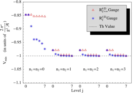
(23) -0.8 D R6Ξ=¥ Gauge. Vmin. 2 Π2 Hin units of L g2 A. -0.85. R4Ξ D Gauge Th Value. -0.9 -0.95 -1 n1 =n2 =1. n1 =n2 =2. n1 =n2 =3. -1.1 0. 7. 0. 7 0 Level j. 7. 0. 7. Figure 1: Values of the minimum of the scalar potential as heavier degrees of freedom are included. 6D Triangles (stars) represent the numerical results obtained in the Rξ=∞ (Rξ4D ) gauge. The horizontal dashed line represents the theoretically predicted value for the potential minimum, in the non-trivial ’t Hooft flux case.. In this simplified example, only the charged scalar (i.e.the tachyon) acquires a non vanishing vacuum expectation value (vev ) while the neutral fields remain unshifted. Using the (4) numerical value 1/I0 = (0.85 A), it results:10 Vmin = −. 2H2 (4). g2 I0. ∼ −0.85 ×. 2π 2 , g2 A. (4.5). which is still quite different from that predicted by eq. (4.2). Moreover, it is enough to add the interactions with either the next neutral or charged levels to observe the appearance of tadpole terms. That is, the true minimum of the system does not correspond then anymore to the vev s obtained in eq. (4.4), but all fields get new shifts instead. We found that generically all charged and neutral fields in the two towers get vev s. Figure (1) shows the dynamical approach to the true minimum by the successive addition of heavier charged modes (labelled by j = 0, . . . , 7 in the horizontal axis) and heavier 6D gauges. neutral modes (labelled with n1 = n2 = 0, . . . , 3), for both the Rξ4D and Rξ=∞ For example, the point labelled with n1 = n2 = 1 and j = 3 represents the numerical calculation where all degrees of freedom up to n1 = n2 = 1 and j = 3 are included. The graphic shows that the value of the minimum of the scalar potential does converge to the theoretically predicted value of −2π 2 /(g2 A): for n1 = n2 ≥ 1 (≥ 5 neutral complex fields) 10. (4). The dimensions of the quantities in eq. (4.4) are [H] = [I0 ] = [E 2 ] and [g] = [E −1 ].. – 21 –. JHEP01(2007)005. n1 =n2 =0. -1.05.

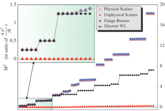
(24) 0.6 D R6Ξ=¥ gauge. M2. 4 Π2 Hin units of L A. 0.5. R4Ξ D gauge Th Value. 0.4. 0.3. 0.2. n1 =n2 =0. n1 =n2 =1. n1 =n2 =2. n1 =n2 =3. 0. 0. 7. 0. 7 0 Level j. 7. 0. 7. Figure 2: Lightest gauge mode mass. Triangles (stars) represent the numerical results obtained 6D in the Rξ=∞ (Rξ4D ) gauge. The horizontal dashed line represents the theoretically predicted value in the non-trivial ’t Hooft flux case.. and j ≥ 3 (≥ 4 charged complex fields) a precision over 1% is achieved, in both gauges; for 6D n1 = n2 = 3 and j = 7, it reaches 10−5 (10−7 ) for the Rξ=∞ (Rξ4D ) gauge. As regards the symmetries of the spectrum, the numerical results confirm that the SU(2) symmetry is completely broken. This is well illustrated by figure 2, where the lightest vector state is shown to be asymptotically massive. The horizontal dashed line represents the mass value of 0.25 (in units of 4π 2 /A), theoretically predicted in eq. (2.35). An excellent agreement is observed as well between the calculations in the two gauges after the levels up to n1 = n2 ≥ 1 and j ≥ 3 are included. We have thus explicitly proved that the SU(2) symmetry is completely broken. In figure 3 the full spectrum of the 4D vector fields is displayed, with all fields up to 6D n1 = n2 = 3 and j = 7 included in the estimation, in the Rξ4D and Rξ=∞ gauges. No visible difference can be noticed. This result is a strong numerical proof of the consistency of our effective 4D Lagrangian, and its manifest gauge invariance when a sufficient number of heavy degrees of freedom are included. Finally, figure 4 retakes the full spectrum, resulting from the diagonalization of the complete system, in the Rξ4D gauge: gauge bosons (stars), physical scalars (empty triangles) and unphysical scalars (full triangles), with the latter corresponding to the choice ξ = 0. Superimposed, the figure shows as well (black dots joined by a full line) the theoretical prediction for constant discrete Scherk-Schwarz boundary conditions, eq. (2.35). Notice that:. – 22 –. JHEP01(2007)005. 0.1.

(25) 20 D j=7, n1 =n2 =3 - R6Ξ=¥ gauge. 15. 10. 5. 0. 10. 20. 30 Modes. 40. 50. 60. Figure 3: Gauge invariance of the gauge spectrum for the non-trivial ’t Hooft flux case. Triangles 6D (stars) represent the numerical results obtained in the Rξ=∞ (Rξ4D ) gauge respectively, for n1 = n2 = 3 and j = 7.. • Each 4D vector boson has a physical scalar partner degenerate in mass, as expected in the asymptotic limit from eqs. (3.46) and (3.48). • The unphysical scalar spectrum -which constitutes half of the scalar spectrum- is identified as those fields which appear to have zero mass, as expected for “pseudogoldstone bosons” eaten by the vector fields to acquire masses.11 A slight numerical mismatch only appears for the masses of the pseudo-goldstone fields of the heavier modes, as the numerical truncation of the tower of states starts to be felt • The coincidence between the numerical results -obtained with y-dependent boundary conditions- and the spectrum predicted for constant discrete Scherk-Schwarz boundary conditions (black dots) is very good up to the first 20 modes (i.e. around M 2 ≈ 3 in the units chosen for illustration). The agreement of the overall scale, as well as the expected four-fold degeneracy of the first two massive levels and the eight-fold degeneracy of the next one, are clearly seen. Only the higher levels start to show disagreement with the theoretical formulas. This is as it should be, as the present numerical analysis was restricted to charged levels up to j = 7 and neutral ones up to n1 = n2 = 3. Indeed, the next mode non-included in the numerical analysis would 11. As stated, this numerical spectrum has been computed for ξ = 0, but it can also be viewed as corresponding to the ξ-independent contributions to the goldstone masses for any ξ, as it follows from eq. (3.48).. – 23 –. JHEP01(2007)005. M2gauge. 4 Π2 Hin units of L A. j=7, n1 =n2 =3 - R4Ξ D gauge.

(26) be j = 8, which has a squared mass M 2 ≈ 2.7. In consequence, the numerical results and the theoretical prediction start to diverge around this scale. The mode j = 8 sets the limit of validity of the present numerical analysis, while a better agreement can be reached including higher modes. We have also computed the physical spectrum in the Rξ4D gauge by another procedure: the direct substitution of the vev s obtained from the numerical minimization into the total covariant derivatives in eqs. (3.46) and (3.48). The coincidence with the numerical results shown above is so precise that it would be indistinguishable within the drawing precision. 4.2 Trivial ’t Hooft flux: m = 0, k = 1 Consider now the case of trivial ’t Hooft flux, in which the generators of the translation operators Ti commute. The simplest non-trivial configuration of this type12 corresponds to m = 0 and k = 1. A two-fold degeneracy of the charged (Landau) levels is then present, as d = 2 in eq. (3.40) and ρ = 0, 1. In consequence, due to the higher number of states, the numerical treatment is more cumbersome than in the previous Subsection. The dynamical approach to the minimum of the 4D potential can be seen in figure 5. Again it shows how the asymptotic regime is reached with the successive addition of heavier charged and neutral fields. The dashed horizontal line represents the theoretical predicted 12. That is, with lowest degeneracy.. – 24 –. JHEP01(2007)005. 4D Figure 4: Full spectrum for the non-trivial ’t Hooft flux case, in the Rξ=0 -gauge. Gauge bosons (stars), physical scalars (empty triangles) and unphysical scalars (full triangles) are shown. The minimization procedure includes all charged and neutral modes up to n1 = n2 = 3 and j = 7. Black dots joined by a full line represent the theoretically predicted masses derived in section 2.2..

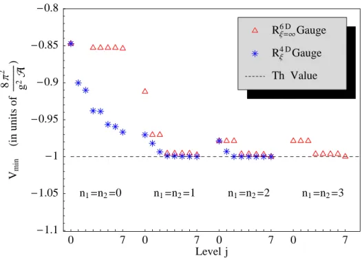
(27) -0.8 D R6Ξ=¥ Gauge. Vmin. 8 Π2 Hin units of L g2 A. -0.85. R4Ξ D Gauge Th Value. -0.9 -0.95 -1 n1 =n2 =1. n1 =n2 =2. n1 =n2 =3. -1.1 0. 7. 0. 7 0 Level j. 7. 0. 7. Figure 5: Values of the minimum of the scalar potential as heavier degrees of freedom are included. 6D Triangles (stars) represent the numerical results obtained in the Rξ=∞ (Rξ4D ) gauge. The horizontal dashed line represents the theoretically predicted value for the potential minimum, in the trivial ’t Hooft flux case.. value, −8π 2 /g2 A, as expected from eq. (4.2): for n1 = n2 ≥ 1 (≥ 5 neutral fields) and 6D gauge and in j ≥ 3 (≥ 4 charged fields) a precision over 1% is achieved, both in the Rξ=∞ 6D the Rξ4D gauge. In the best case that we could numerically evaluate for the Rξ=∞ gauge −5 (n1 = n2 = 3, j = 7), a precision of O(10 ) has been obtained. As regards the expected spectra, recall from Subsection 2.1 that all possible solutions should correspond to either unbroken SU(2) symmetry or a SU(2) → U(1) breaking patterns, all of them being degenerate in the absence of quantum corrections and fermions. All numerical results obtained here turn out to correspond to SU(2) → U(1) breaking examples. This is well illustrated by figure 6 where the mass of one (and only one) vector state is seen to vanish asymptotically, in agreement with the lightest value predicted in eq. (2.25) for αi 6= 0. That state is the 4D gauge vector boson of the unbroken U(1) symmetry. The figure also shows clearly that if only the first few light levels of the KK and Landau towers would have been considered in the analysis, the lightest state would have looked massive, suggesting a fake SU(2) → ∅ breaking pattern. Only the inclusion of higher charged and neutral levels allows to attain the asymptotic regime, unveiling then the remaining U(1) symmetry. Numerically, the agreement with the theoretical prediction starts to be satisfactory for n1 = n2 ≥ 1 and j ≥ 3, analogously to the case with non-trivial ’t Hooft flux in the previous Subsection. It is worth pointing out that the U(1) symmetry of the total stable vacuum selects,. – 25 –. JHEP01(2007)005. n1 =n2 =0. -1.05.

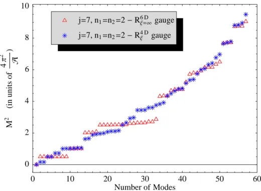
(28) 0.6 D R6Ξ=¥ gauge. R4Ξ D gauge Th Value. 0.4. n1 =n2 =0. 0.3 n1 =n2 =1. 0.2. M2. 4 Π2 Hin units of L A. 0.5. n1 =n2 =2 n1 =n2 =3. 0 0. 7. 0. 7 0 Level j. 7. 0. 7. Figure 6: Lightest gauge mode mass. Triangles (stars) represent the numerical results obtained 6D in the Rξ=∞ (Rξ4D ) gauge. The horizontal dashed line represents the theoretically predicted value in the trivial ’t Hooft flux case.. in general, a different gauge direction, in SU(2) space, than that of the imposed abelian background. In other words, it may be a different U(1) symmetry than that naively exhibited by the Lagrangian, when expanded around the imposed background. The neutral and charged towers of fields, as defined by the latter, have recombined dynamically, to select the final stable symmetric direction. Figure 7 shows two gauge spectra obtained numerically including all modes up to 6D n1 = n2 = 2 and j = 7, for the two gauges Rξ=∞ (triangles) and Rξ4D (stars). Notice the difference with the analogous figure obtained for the m = 1 case, figure 3: at first sight, one could think that the test of gauge invariance fails in the present case. This is not the case, though: the two spectra turn out to correspond to different values for the set of arbitrary parameters α1 , α2 , in eq. (2.27), which parametrize the possible ScherkSchwarz spectra. We determined the values chosen by the minimization algorithm in these examples, performing a two-parameter fit to the first 20 masses obtained from the numerical procedure. The χ2 value of the fit is extremely significant for both gauges. It resulted in 6D gauge, as can be easily the values α1 = α2 = 1/2 for the example shown in the Rξ=∞ deduced from the observed boson multiplicity. Conversely, for the Rξ4D gauge calculation, the minimization algorithm selected α1 = 0.334 and α2 = 0.219, to which it corresponds the observed lower multiplicity of degenerate fields. Examples corresponding to other values have also been obtained, although not illustrated here. The existence of different spectra for the same symmetry breaking pattern is generic of Scherk-Schwarz compactification at. – 26 –. JHEP01(2007)005. 0.1.

(29) 10 D j=7, n1 =n2 =2 - R6Ξ=¥ gauge. j=7, n1 =n2 =2 - R4Ξ D gauge. 6. 4. M2. 4 Π2 Hin units of L A. 8. 0 0. 10. 20. 30 40 Number of Modes. 50. 60. Figure 7: Gauge boson spectra for the trivial ’t Hooft flux case. Triangles (stars) represent the 6D numerical results obtained in the Rξ=∞ (Rξ4D ) gauge respectively, for n1 = n2 = 2 and j = 7. In this example, the two spectra turn out to correspond to different sets of (α1 , α2 ) values: (1/2, 1/2) (triangles) and (0.33, 0.22) (stars).. the classical level. In figure 8 we retake the gauge (stars), physical scalar (empty triangles) and unphysical scalar ( full triangles) spectra, in the Rξ4D gauge, for the same αi values than in the previous figure, and with the unphysical scalar masses computed for ξ = 0. Due to the degeneracy of the Landau levels, the numerical analysis could only be performed including modes up to n1 = n2 = 2 and j = 7. The masses of the unphysical scalar degrees of freedom tend, as before, to vanish -as they should- as the asymptotic regime is approached. For the heavier modes, a slight numerical mismatch appears between the masses of the vector fields and those of their physical scalar partners. A corresponding tiny mass for the unphysical scalar partners is also observed. This discrepancy is again consequence of the truncation error. Apart form this subtlety, physical scalar and gauge masses are in excellent agreement. Moreover, the agreement between the numerical spectra and the theoretically predicted one - typical of Scherk-Schwarz breaking and represented in figure 8 with black dots joined by a full line - is very good up to the first 40 modes (i.e.around M 2 ≈ 4 in the units chosen). This scale sets the validity limit for the present numerical analysis of our lowenergy effective 4D theory. A better agreement above this scale could be obtained adding higher modes. Once again, the mass of the next non-included mode, the j = 8 mode, is M 2 ≈ 5.4 and coincides with the scale at which the numerical masses and the theoretical predicted ones start to diverge.. – 27 –. JHEP01(2007)005. 2.

(30) Finally, we have also computed the physical spectrum in the Rξ4D gauge by another procedure: the direct substitution of the vev s obtained from the numerical minimization into the total covariant derivatives in eqs. (3.46) and (3.48). The coincidence with the numerical results shown above is so precise that it would be indistinguishable within the drawing precision. In summary, in this section we have thus explicitly shown, for the 6D SU(2) gauge group compactified on a 2D torus, that a stable vacuum of zero energy is reached, out of the initial unstable configuration. To solve the system with y-dependent boundary conditions has been shown to be tantamount to solve it with constant boundary conditions. For the case of non-trivial ’t Hooft flux, the pattern of symmetry breaking obtained is SU(2) −→ ∅ and it corresponds to Scherk-Schwarz symmetry breaking with discrete Wilson lines. For trivial ’t Hooft flux, the patterns found correspond to SU(2) −→ U(1) and are equivalent to Scherk-Schwarz symmetry breaking with continuous Wilson lines.. 5. Conclusions and outlook Boundary conditions depending upon the extra coordinates are equivalent to constant ones, for SU(N ) on a two-dimensional torus. For trivial ’t Hooft flux, they are equivalent to constant Scherk-Schwarz boundary conditions, associated to continuous Wilson lines. For. – 28 –. JHEP01(2007)005. Figure 8: Numerical results for the trivial ’t Hooft flux case, in the Rξ4D -gauge. Gauge bosons (stars), physical scalars (empty triangles) and unphysical scalars (stars) are shown. The minimization procedure includes all the charged and neutral modes up to n1 = n2 = 2 and j = 7. Black dots joined by a full line represent the theoretically predicted masses derived in section 2.1, for the case α1 = 0.33, α2 = 0.22..

(31) Acknowledgments We are indebted for very interesting discussions to E. Alvarez, J. Barbon, J. Bellorı́n,. – 29 –. JHEP01(2007)005. the case of non-trivial ’t Hooft flux, the coordinate-dependent boundary conditions can be traded instead by constant Scherk-Schwarz boundary conditions, associated to discrete Wilson lines, resulting always in symmetry breaking. One of the novel features of this work is the study of the phenomenological implications of this last scenario, studying the pattern of gauge symmetry breaking and the spectrum of the four-dimensional vector and scalar excitations. Chirality cannot be implemented within a SU(N ) background and will require to consider in the future non-simply connected groups. For them, the equivalence between coordinate-dependent and constant boundary conditions does not hold in general. A fieldtheory treatment of the system subject to coordinate dependent boundary conditions is then necessary to solve the details of the four-dimensional spectrum. We start this approach in the present work by treating also explicitly the case of SU(2) on a torus with background. We have explicitally solved the Nielsen-Olesen instability on the two dimensional torus. For the obtention of the four-dimensional effective Lagrangian, all couplings have been taken into account, including all quartic and cubic terms mixing Kaluza-Klein and Landau levels. Those terms are shown to be essential in the determination of the stable minimum of the potential and its symmetries. The corresponding integrals over the extra-dimensional space have been obtained analytically for all modes, for the first time. Furthermore, we have defined gauge-fixing Lagrangians, appropiate when both Kaluza-Klein and Landau levels are simultaneously present and interacting. We found that the naive Rξ gauge defined in six dimensions is then not equivalent to the Rξ gauge in four dimensions. The computations have been performed in different possible gauge choices and the issue has been clarified in depth. These technical tools will be necessary when groups other than SU(N ) will be considered. The system is seen to evolve dynamically from the unstable background configuration towards a stable and non-trivial background of zero energy. This happens through an infinite chain of vacuum expectation values of the four-dimensional scalar fields. The resulting spectra do show explicitly the symmetries expected from the theoretical analysis mentioned above, for the case of SU(N ) with constant boundary conditions. It turns out that for each four-dimensional gauge boson there exists a scalar partner degenerate in mass, both for trivial and non-trivial ‘t Hooft fluxes. This is one of the important phenomenological drawbacks that the approach has to face. The scenario has to be enlarged then, for instance including more than just one scale in the theory. Indeed, a motivation for the present work was the hypothetical identification of the Higgs field as a component of a gauge boson in full space, which would make its mass insensitive to ultraviolet contributions, unlike in the Standard Model. To find a realistic pattern of electroweak symmetry breaking, which matches the spectra found in nature, remains a non-trivial issue..