Modelado en dinámica de fluidos computacional (CFD) de transporte de masa en materiales porosos
76
0
0
Texto completo
(2) TFG REALIZADO EN PROGRAMA DE INTERCAMBIO. TÍTULO:. CFD modeling of mass transport in porous materials. ALUMNO:. Miguel Hernández Blanco. FECHA:. 12.07.2017. CENTRO:. Institut für Energietechnik, Professur für Technische Thermodynamik. TUTOR:. Prof. Dr. Cornelia Breitkopf.
(3) Resumen La difusión y la adsorción son fenómenos complejos que ocurren durante las reacciones catalíticas de forma acoplada y en función del tiempo. Estos procesos pueden ser estudiados mediante un análisis microcinético. Un método para realizar este análisis es el uso de un aparato de Respuesta por Frecuencia (FR). El objetivo de este proyecto es la creación de un modelo, utilizando el software de simulación COMSOL Multiphysics, que recree un experimento FR en el que un gas es comprimido y expandido periódicamente para favorecer la difusión y adsorción en un material poroso. Diferentes variables han de tenerse en cuenta, centrándose este proyecto en la simulación del material poroso – el catalizador – y los procesos de transporte de masa, además del correcto cálculo de campos de presión y velocidad, y transferencia de calor. Finalmente, se presenta un estudio de los resultados de la evolución del experimento, obtenidos del modelo computacional final.. Palabras Clave Difusión – Adsorción – Material poroso – Respuesta por Frecuencia – COMSOL Multiphysics. Abstract Diffusion and adsorption are complex phenomena which occur during catalytic reactions as coupled and time dependent processes. These processes can be studied by realizing a microkinetic analysis. One method to achieve this is by using a Frequency Response (FR) apparatus. The objective of this project is the creation of a model – using the simulation software COMSOL Multiphysics – which recreates a FR experiment in which a gas is periodically compressed and expanded to favor diffusion and adsorption in a porous material. Several variables are to be taken into account, being this project focused on the simulation of the porous material – the catalyst – and the processes of mass transport, as well as on the correct calculation of pressure and velocity fields, and heat transfer. To conclude, a study of the results of the evolution of the experiment, obtained from the final computational model, is presented.. Keywords Diffusion – Adsorption – Porous material – Frequency Response – COMSOL Multiphysics.
(4) Fakultät Maschinenwesen Institut für Energietechnik, Professur für Technische Thermodynamik. CFD modeling of mass transport in porous materials Bachelor Thesis. Miguel Hernández Blanco Betreuender Hochschullehrer: Prof. Dr. Cornelia Breitkopf Bearbeitungszeitraum: 03.2017 – 07.2017.
(5) Table of Contents Table of Figures............................................................................................................................................. II List of Tables ............................................................................................................................................... III Abbreviations and Symbols......................................................................................................................... IV 1 Introduction ................................................................................................................................................ 1 2 Objectives ................................................................................................................................................... 2 3 Theory ........................................................................................................................................................ 3 3.1 Laminar Flow ...................................................................................................................................... 3 3.2 Heat Transfer ....................................................................................................................................... 4 3.3 Transport of Diluted Species in Porous Media.................................................................................... 5 4 Frequency Response Method ..................................................................................................................... 8 5 Experimental Setup .................................................................................................................................. 10 6 Computational Setup using COMSOL Multiphysics ............................................................................... 12 6.1 Definition of Parameters ................................................................................................................... 12 6.2 Simulation of the Frequency Response Input .................................................................................... 14 7 Geometry .................................................................................................................................................. 17 8 Materials ................................................................................................................................................... 22 9 Interfaces .................................................................................................................................................. 26 9.1 Laminar Flow 1 ................................................................................................................................. 26 9.2 Laminar Flow 2 ................................................................................................................................. 31 9.3 Moving Mesh .................................................................................................................................... 34 9.4 Heat Transfer in Solids ...................................................................................................................... 38 9.5 Transport of Diluted Species in Porous Media.................................................................................. 41 10 Mesh ....................................................................................................................................................... 47 11 Simulation Study Settings ...................................................................................................................... 53 12 Results .................................................................................................................................................... 55 12.1 Simplification of the Geometry ....................................................................................................... 55 12.2 Concentration of the Inner Fluid in the Porous Material ................................................................. 57 12.3 Pressure Response affected by Mass Transport .............................................................................. 62 13 Summary and Conclusions ..................................................................................................................... 65 14 Bibliography ........................................................................................................................................... 66 I.
(6) Table of Figures Figure 1: Fundamental concept of frequency response analysis. Taken from [4]. ........................................ 8 Figure 2: Experimental setup for Frequency Response ............................................................................... 10 Figure 3: Detailed view to volume modulation unit of FR.......................................................................... 11 Figure 4: Main parameters of the sinusoidal function of displacement....................................................... 14 Figure 5: Sinusoidal function of displacement, wave (x) ............................................................................ 15 Figure 6: Main parameters of the square function of displacement ............................................................ 16 Figure 7: Square function of displacement, wave (x) .................................................................................. 16 Figure 8: Interior geometry of the model .................................................................................................... 18 Figure 9: Complete previous geometry of the model .................................................................................. 19 Figure 10: Detail of the new geometry ........................................................................................................ 20 Figure 11: Complete current geometry of the model .................................................................................. 20 Figure 12: ‘Add Material’ window.............................................................................................................. 22 Figure 13: Carbon dioxide domains ............................................................................................................ 23 Figure 14: Air domains................................................................................................................................ 23 Figure 15: Steel AISI 4340 domains ........................................................................................................... 24 Figure 16: Glass domain.............................................................................................................................. 24 Figure 17: Material Contents table for the Zeolite 5A ................................................................................ 25 Figure 18: Zeolite 5A domain ..................................................................................................................... 25 Figure 19: ‘Add Physics’ window ............................................................................................................... 26 Figure 20: Laminar Flow 1 domains ........................................................................................................... 27 Figure 21: Laminar Flow 1 reference values ............................................................................................... 27 Figure 22: Laminar Flow 1 model inputs and fluid properties .................................................................... 28 Figure 23: ‘No Slip Wall’ boundaries ......................................................................................................... 28 Figure 24: Example of the settings of a Linear Extrusion ........................................................................... 29 Figure 25: Example of the settings of a ‘Moving Wall’ in Laminar Flow 1 ............................................... 30 Figure 26: Settings and selected boundary of the ‘Pointwise Constraint’ ................................................... 31 Figure 27: ‘Laminar Flow 2’ domains......................................................................................................... 32 Figure 28: Laminar Flow 2 model inputs and fluid properties .................................................................... 32 Figure 29: Example of the settings of a ‘Moving Wall’ in Laminar Flow 2 ............................................... 33 Figure 30: Settings and selected boundaries of ‘Open Boundary’ in Laminar Flow 2 ............................... 34 Figure 31: ‘Moving Mesh’ domains ............................................................................................................ 35 Figure 32: Settings and selected boundaries of Prescribed Mesh Displacement 1...................................... 36 Figure 33: Settings and selected boundaries of Prescribed Mesh Displacement 2...................................... 37 Figure 34: Settings and selected boundaries of Prescribed Mesh Displacement 3...................................... 37 Figure 35: ‘Solid’ node domains ................................................................................................................. 38 Figure 36: ‘Thermal Insulation’ boundary .................................................................................................. 39 Figure 37: Settings and selected boundaries of ‘Open Boundary’ in Heat Transfer ................................... 39 Figure 38: ‘Thin Thermally Resistive Layer’ boundaries ........................................................................... 41 Figure 39: ‘Transport of Diluted Species’ domain ...................................................................................... 42 Figure 40: Selection of ‘Adsorption’ in the Transport Mechanisms section ............................................... 42 Figure 41: ‘Matrix properties’ settings ........................................................................................................ 43 Figure 42: ‘Diffusion’ settings .................................................................................................................... 43 II.
(7) Figure 43: ‘Adsorption’ settings.................................................................................................................. 44 Figure 44: ‘No Flux’ boundaries ................................................................................................................. 45 Figure 45: Settings and selected boundary of ‘Inflow’ ............................................................................... 46 Figure 46: Free Triangular Mesh in the main heat exchange zone domains ............................................... 47 Figure 47: Free Triangular Mesh settings ................................................................................................... 48 Figure 48: Results comparison for velocity of the outer fluid. Former vs. new geometry and mesh. Smoother evolution of the results in the second case. ................................................................................. 49 Figure 49: Free Quad Mesh domains .......................................................................................................... 50 Figure 50: Free Quad Mesh settings ............................................................................................................ 50 Figure 51: Free Triangular Mesh in the reactor domains ............................................................................ 51 Figure 52: Former vs. new mesh comparison in the reactor ....................................................................... 51 Figure 53: Concentration results comparison. Former vs. new mesh. Smoother evolution of the results in the second case. ........................................................................................................................................... 52 Figure 54: ‘Boundary Layers’ boundaries ................................................................................................... 52 Figure 55: Selection of ‘Study 2, Stationary’ in the ‘Time Dependent Study’ settings .............................. 54 Figure 56: Comparison of the maximum temperature over time. Former vs. new geometry. The temperature peak is reached at the same time instant t=0.056 s. ................................................................. 56 Figure 57: Comparison of the graphihc results of temperature for the instant t=0.056 s. Fromer vs. new geometry. The maximum temperature is reached in both cases at the centre of the lower part of the volume-modulation unit .............................................................................................................................. 56 Figure 58: Pressure evolution in the reactor ................................................................................................ 57 Figure 59: Inner fluid concentration in the porous material. Evolution over time ...................................... 58 Figure 60: Concentration of the inner fluid in the porous material at t=0 ................................................... 59 Figure 61: Concentration of the inner fluid in the porous material at t=0.025 s ......................................... 59 Figure 62: Concentration of the inner fluid in the porous material at t=0.05 s ........................................... 60 Figure 63: Concentration of the inner fluid in the porous material at t=0.075 s ......................................... 60 Figure 64: Concentration of the inner fluid in the porous material at t=0.1 s ............................................. 61 Figure 65: Pressure graphic results for instants of maximum and minimum volume under the travel plate ..................................................................................................................................................................... 63 Figure 66: Pressure evolution in the reactor. Case with no concentration variation effect vs. case with concentration variation influence on the pressure ....................................................................................... 64. List of Tables Table 1: Parameterized variables in COMSOL Multiphysics ..................................................................... 13 Table 2: Simulation times comparison. Former vs. new geometry and mesh ............................................. 49 Table 3: Pressure in the reactor comparison for instants of maximum and minimum volume under the travel plate ................................................................................................................................................... 63. III.
(8) Abbreviations and Symbols FR. Frequency Response. spf. Laminar Flow. ale. Moving Mesh. ht. Heat Transfer in Solids. tds. Transport of Diluted Species in Porous Media. 𝑐𝑐 [ 𝑐𝑖 [. 𝑚𝑜𝑙. ]. species inflow of gas into the reactor. ]. concentration of species i in the liquid phase. 𝑚3. 𝑚𝑜𝑙 𝑚3. 𝑐𝐺,𝑖 [ 𝑐𝑃,𝑖 [. 𝑚𝑜𝑙. ]. concentration of species i in the gas phase. ]. amount of species i adsorbed or desorbed from the solid particles. 𝑚𝑜𝑙. adsorption maximum. 𝑚3. 𝑚𝑜𝑙 𝑚3. 𝑐𝑃𝑚𝑎𝑥 [ 𝐾𝑔 ] 𝑐0 [. 𝑚𝑜𝑙 ] 𝑚3. initial concentration of fluid in the porous material. 𝐽 ] (𝐾𝑔∙𝐾). specific heat capacity at constant pressure. 𝐶𝑝 [ D[. 𝑚2 ] 𝑠. Diffusion coefficient. 𝑁. volume force vector. 𝐅 [𝑚 3 ] 𝑚3. 𝐾𝐿 [𝑚𝑜𝑙]. Langmuir constant. 𝑝 [Pa]. pressure. 𝑝𝐴 [Pa]. absolute pressure of the spf interface. 𝑃𝑠𝑝𝑓 [Pa]. pressure of the spf interface. 𝑃0 [Pa]. initial pressure in the reactor. 𝑊. 𝐪 [𝑚 2 ] 𝑊. 𝐪𝐫 [ 𝑚 2 ] 𝑊. 𝑄 [𝑚3 ] 𝑊. 𝑄𝑝 [𝑚3 ]. heat flux vector heat flux by radiation heat sources work done by pressure changes. IV.
(9) 𝑊. 𝑄𝑣𝑑 [𝑚3 ] 𝐽. R [𝐾𝑔·𝐾]. viscous dissipation in the fluid universal gas constant. 𝑅𝑖 [𝑚3 ·𝑠]. 𝑚𝑜𝑙. reaction rate expression for the species i. 𝑆𝑖 [𝑚3 ·𝑠] t [s]. 𝑚𝑜𝑙. arbitrary source term for the mass balance equation. 𝑇 [K]. temperature. 𝑇0 [K]. initial temperature of gas in the reactor. 𝑚. 𝐮 [𝑠] 1. time. velocity vector. 𝛼𝑝 [𝐾]. coefficient of thermal expansion. 𝜀𝑝 [-]. porosity. Θ [-]. liquid volume fraction. 𝜇 [Pa·s]. dynamic viscosity. V.
(10) 1 Introduction Adsorption and diffusion are two complex phenomena which occur during catalytic reactions as coupled and time dependent processes. A catalyst is a substance which, when added to a reaction, increases the rate of the reaction without being consumed or produced in it. Catalysts can be homogeneous – they operate in the same phase which reactants and products have, – and heterogeneous – they operate in a different phase, usually solid [1]. Zeolites are one special type of heterogeneous catalyst. A zeolite is a porous crystalline aluminosilicate. It consists of regular arrangements of SiO4 and AlO4 tetrahedra, which form a crystal structure through shared oxygen atoms [2]. Although zeolites can be found in nature, it was not until the synthetic zeolites appeared that these porous materials started having an important role as catalysts. The molecular dimensions size of the pores of a zeolite presents a range 0.3 to 2.0 nm, being thus considered microporous materials [3]. In order to characterize zeolites, a microkinetic analysis can be made. In this microkinetic analysis, the conditions of diffusion and adsorption in catalytic reactions are studied. One of the methods to achieve this is by using a Frequency Response (FR) apparatus. The FR experiment consists of varying the volume of the system and measuring and studying the pressure response. This volume modulation compresses and expands the inner fluid towards the porous material, and favors the sorption and diffusion processes [4]. During the FR experiment many variables are to be taken into account. The main focus is to study the adsorption and diffusion processes, but other aspects such as the behavior of the fluid, the materials of which the setup is made of, or the outer gas, have an influence due to the variation of pressure, velocity fields, temperature or mass transport. In order to perform and evaluate a FR experiment, computer simulations can be used. They present several advantages, such as a significant saving of time and resources, and the possibility to recreate quite exactly the conditions of the experiment and the laboratory. It is possible to describe the experiment in this way, and in addition, this description can be later modified in order to repeat the experiment with different settings. For this project, the used simulation tool is the software COMSOL Multiphysics 5.2a.. 1.
(11) 2 Objectives The main aim of the experiment using the FR apparatus is to study the time dependent processes of adsorption and diffusion, and this study can be made recreating the real experiment with a simulation tool. Therefore, the principal objective of this project is the creation of a model using the software COMSOL Multiphysics 5.2a to simulate those coupled processes of adsorption/desorption and diffusion. This will facilitate the study and characterization of zeolites to know more about the kinetics of adsorption and diffusion, using a simulation software to reduce the study time. An existing model based on the real FR experiment was taken as a starting point for this project [5]. The goals of this current project consist of improving the previous model and implementing the interfaces and settings needed to simulate the mass transport in porous materials. It is intended for the model to become a more complete and optimized simulation, so that results can be more accurately and rapidly obtained with the computational model, and so that they can be later compared with the real experimental results. This way, one major aim is to make the model become more complete regarding the description of the porous material and the mass transport. It is also intended to make the model result in a more detailed recreation of the real experiment. This will provide the possibility to help future projects – both focused on this topic or not – as the settings of the model can be changed to have more possible uses in the future.. 2.
(12) 3 Theory In this chapter, the different equations which the software COMOSL Multiphysics solves for the simulation of this project will be discussed. The model describes the conditions of the experiment, and several interfaces need to be implemented to recreate the real processes which affect the porous material, the inner fluid, and the environment.. 3.1 Laminar Flow This interface, as well as the rest of the Single Phase Fluid Flow ones, is based on the Navier-Stokes equations, which in their general form are: The continuity equation, which represents the conservation of mass: ∂𝜌 + ∇ ∙ (𝜌𝐮) = 0 ∂t. (Eq. 1). The equation for conservation of momentum, which is a vector equation: 𝜌. ∂𝐮 + 𝜌 (𝐮 ∙ ∇)𝐮 = ∇ ∙ [− 𝑝𝐈 + 𝝉] + 𝐅 ∂t. (Eq. 2). And the equation for conservation of energy: 𝜕𝑇 𝑇 𝜕𝜌 𝜕𝑝 𝜌𝐶𝑝 ( + (𝐮 ∙ ∇)𝑇) = −(∇ ∙ 𝐪) + 𝝉: 𝐒 − | ( + (𝐮 ∙ ∇)𝑝) + 𝑄 𝜕𝑡 𝜌 𝜕𝑇 𝑝 𝜕𝑡. (Eq. 3). Being S the strain rate tensor: 1 𝐒 = (∇𝐮 + (∇𝐮)𝑇 ) 2. (Eq. 4). A Newtonian fluid presents a linear relation between stress and strain [6]. In this case, the viscous stress tensor adopts the following expression: 2 𝝉 = 2μ𝐒 − μ(∇ ∙ 𝐮)𝐈 3. 3. (Eq. 5).
(13) And more specifically, the motion equations for a single-phase fluid in the case of compressible flow are: The continuity equation for conservation of mass: ∂𝜌 + ∇ ∙ (𝜌𝐮) = 0 ∂t. And the equation for conservation of momentum: 𝜌. ∂𝐮 2 + 𝜌𝐮 ∙ ∇𝐮 = −∇𝑝 + ∇ ∙ (μ(∇𝐮 + (∇𝐮)𝑇 ) − μ((∇ ∙ 𝐮)𝐈) + 𝐅 ∂t 3. (Eq. 6). These equations can be applied to incompressible flow and compressible flow when there are variations of density and viscosity.. 3.2 Heat Transfer The interface responsible for heat transfer is based on the heat equation, which in the case of heat transfer in fluids has the following form [7]: 𝜕𝑇 𝜕𝑝 𝜌𝐶𝑝 ( + 𝐮 ∙ ∇𝑇) + ∇ ∙ (𝐪 + 𝐪𝐫 ) = 𝛼𝑝 𝑇 ( + 𝐮 ∙ ∇p) + 𝜏: ∇𝐮 + 𝑄 𝜕𝑡 𝜕𝑡. (Eq. 7). Being the coefficient of thermal expansion: 𝛼𝑝 = −. 1 𝜕𝜌 𝜌 𝜕𝑇. (Eq. 8). The terms at the right side of the equation represent the different heat sources, which are: The work done by changes of pressure which affects the temperature of the fluid:. 𝜕𝑝 𝑇 𝜕𝜌 𝜕𝑝 𝑄𝑝 = 𝛼𝑝 𝑇 ( + 𝐮 ∙ ∇𝑝) = − ( + 𝐮 ∙ ∇𝑝) 𝜕𝑡 𝜌 𝜕𝑇 𝜕𝑡. 4. (Eq. 9).
(14) The viscous dissipation in the fluid, representing the heat source coming from the transformation of kinetic energy into internal energy due to viscous stresses: 2 𝑄𝑣𝑑 = 𝜏: ∇𝐮 = μ (∇𝐮 + (∇𝐮)𝑇 − (∇ ∙ 𝐮)𝐈) : ∇𝐮 3. (Eq. 10). And finally, the last term (𝑄) represents the external heat source. In this experiment, there is no external heat source, nor difference between the initial temperature of the interior and exterior fluids. Therefore, all the generated heat appears as a consequence of the movement of the fluid, and this las term 𝑄 = 0.. 3.3 Transport of Diluted Species in Porous Media This interface solves the following equation for concentrations to describe the transport of solutes in a variably saturated porous medium, for the most general case: 𝜕 𝜕 𝜕 (𝜃𝑐𝑖 ) + (𝜌𝑏 𝑐𝑃,𝑖 ) + (𝛼𝑉 𝑐𝐺,𝑖 ) + 𝐮 ∙ ∇𝑐𝑖 = ∇ ∙ [(𝐷𝐷,𝑖 + 𝐷𝑒,𝑖 )∇𝑐𝑖 ] + 𝑅𝑖 + 𝑆𝑖 𝜕𝑡 𝜕𝑡 𝜕𝑡. (Eq. 11). The first three terms at the left side of the equation represent the accumulation of species within the liquid, solid and gas phases respectively. The forth term at the left side represents the mass transport due to convection, caused by the velocity field 𝐮. In this general form of the equation: 𝑐𝑖 describes the concentration of species i in the liquid phase. 𝑐𝑃,𝑖 represents the amount of species i adsorbed or desorbed from the solid particles. 𝑐𝐺,𝑖 describes the concentration of species i in the gas phase. The mass transport is balanced by the equation using the porosity 𝜀𝑝 , the liquid volume fraction 𝜃, the bulk density 𝜌𝑏 and the solid phase density 𝜌. In the current experiment, only adsorption of the inner gas on the solid particles of the porous material takes place, as these are the two materials present. Hence, only the term 𝑐𝑃,𝑖 is used. At the right side of the equation, the first term describes the spreading of the species caused by the mechanical mixing and diffusion. The second term is a reaction rate expression, which in this experiment will be 𝑅𝑖 = 0, as no reaction takes place. Finally, the third term, 𝑆𝑖 is an arbitrary source term.. 5.
(15) To solve the diffusion process – the movement of molecules down a concentration gradient – the equation used is Fick’s diffusion equation: 𝜕𝑐 = ∇ ∙ (𝐷∇𝑐) + 𝑅𝑖 𝜕𝑡. (Eq. 12). As no reaction takes place (𝑅 = 0), and the Diffusion coefficient 𝐷 is a constant, it can be expressed as the following: 𝜕𝑐 = 𝐷 ∇2 𝑐 𝜕𝑡. (Eq. 13). To describe the adsorption and desorption processes, adsorption isotherms are used. This process of adsorption consists of the adhesion of molecules from the inner gas to the surface of the porous material. Desorption is the opposite process. Adsorption decreases the concentration of the species in the fluid, while desorption increases it. In this project, the Langmuir isotherm is chosen to describe the amount of species sorbed, being the relation between the solid concentration, 𝑐𝑃 and the concentration in the fluid phase, 𝑐 expressed by the following equations: 𝑐𝑃 = 𝑐𝑃𝑚𝑎𝑥. 𝐾𝐿 𝑐 1 + 𝐾𝐿 𝑐. 𝜕𝑐𝑃 𝐾𝐿 𝑐𝑃𝑚𝑎𝑥 = 𝜕𝑐 (1 + 𝐾𝐿 𝑐)2. (Eq. 14). (Eq. 15). The number of molecules of the species which are being adsorbed, 𝑛+ in a differential time interval, 𝑑𝑡 are directly proportional to the pressure, 𝑝 and the number of empty sites, (𝑁 − 𝑛) which the adsorbent presents: 𝑑𝑛+ = 𝑘 + 𝑝(𝑁 − 𝑛) 𝑑𝑡. (Eq. 16). While the number of molecules which are being desorbed, 𝑛− in this differential time interval, 𝑑𝑡 is proportional to the number of molecules which have been already adsorbed, 𝑛: 𝑑𝑛− = 𝑘−𝑛 𝑑𝑡 Both 𝑘 + and 𝑘 − are positive constants. 6. (Eq. 17).
(16) Therefore, the concentration of the species being adsorbed and desorbed suffers a variation which can be expressed as the following [8]: 𝑑𝑛 = 𝑘 + 𝑝(𝑁 − 𝑛) − 𝑘 − 𝑛 𝑑𝑡. (Eq. 18). Finally, diffusion and adsorption can occur, not only independently, but also as coupled processes. This is the case studied in this project. The porous material is affected by the process of diffusion in the pore voids, and the process of adsorption on the surface. When the rates of both processes are comparable, the equations which describe the coupled processes are the following [9]: 𝜕𝑐 𝜕𝑛 + 𝜌𝑃 = 𝐷 ∇2 𝑐 𝜕𝑡 𝜕𝑡. (Eq. 19). 𝜕𝑛 = 𝑘 + 𝑝(𝑁 − 𝑛) − 𝑘 − 𝑛 𝜕𝑡. (Eq. 20). 7.
(17) 4 Frequency Response Method The Frequency Response (FR) method was originally developed by Polinski and Naphtali in 1963 [10]. Since then, this method has been used to study and measure kinetic parameters corresponding to diffusion and sorption processes occurring in chemical reactions in porous materials, such as microporous solids. The Frequency Response method permits to study coupled adsorption and diffusion processes in catalytic reactions [9]. The basic principle of the FR method consists of applying a periodic perturbation of a physical variable, for example in the form of a sine or square function, to a system in equilibrium. The response to this input is a periodic output which presents the same frequency as the input, but different amplitude and a phase shift [4] .. Figure 1: Fundamental concept of frequency response analysis. Taken from [4].. The amplitude and the phase lag of the response have a direct relation with the thermodynamic and kinetic characteristics of the system. The system could be open or closed [4]. The experiment studied in this project corresponds to the second case, a closed system. The volume modulation is the periodic input, and the studied output is the resulting variation of the pressure. When a closed system containing porous solids experiments a small fluctuation in its volume, the pressure response of the closed system offers information about the rate processes which take place in the porous materials within the system. If the volume fluctuations are small, the interpretation of the response is simpler, as the equilibrium of the system does not suffer significant perturbations [9].. 8.
(18) The calculation of the relevant constants of the studied processes is possible due to the measurement of the phase shift between the input and the output, as well as to the measurement of the amplitude of the output with respect to the amplitude of the input [11]. The results obtained with the FR method – amplitude change and phase shift – have their origin in the dynamics and capacities of the processes which make the system return to its equilibrium point. When diffusion occurs, the effective diffusivity (dynamics) and the pore volume within the porous material (capacity) are responsible for the amplitude change and phase shift of the pressure response. As it was mentioned before, the FR method allows to determine adsorption-desorption and diffusion constants simultaneously. When not only diffusion, but also the adsorption-desorption process occur, the kinetics of adsorption (dynamics) and the surface coverage changes due to the applied perturbation (capacity) have also an influence on the pressure response obtained as the output [9].. 9.
(19) 5 Experimental Setup The major components of which the experimental setup consists of are: A vacuum pump, a vacuummeasuring unit, a pressure-measuring unit, a glass reactor, a volume-modulation unit and two electromagnets. There are blocking valves, which permit to realize the volume modulation in a relatively small volume, consisting of the reactor and the pressure measuring unit.. Figure 2: Experimental setup for Frequency Response. Two of the main parts of the setup will be described and analyzed in this project: The glass reactor and the volume-modulation unit. The inner fluid flows through metal pipes which connect these two parts. The reactor is made of glass and is situated at the bottom part of the setup. It has the same diameter as the connecting tubes. It is isolated to reduce heat losses within it, and it is the part which the gas reaches the last. The volume-modulation unit consists of a magnetic travel plate moved by two identical electromagnets. The travel plate contracts and expands two bellows which move up and down, compressing and expanding the gas towards the reactor. The electromagnets permit to establish a volume modulation closely resembling a square function. The electromagnets are not included in this study because they are not in contact with the other solid parts, and thus have no direct effect on the model. Some other parts of the experiment, which are not included in this model, however play an important role in the experiment, are the following: The pressure-measuring unit measures the absolute pressure. A very exact measurement is required, as the changes in pressure are relatively small, and it must also have a high measuring frequency, due to the rapid movement of the bellows.. 10.
(20) The vacuum pump is a device used to evacuate the container before introducing the gas in it. Another function is avoiding the gas reaching its saturation pressure, once the setup is filled. Finally, the vacuum tubes and blocking valves permit to isolate specific parts of the experiment.. Figure 3: Detailed view to volume modulation unit of FR. Once the cell is evacuated, the gas is inserted and the investigation starts. The gas inlet is found at the top of the experimental setup. The gas is introduced in the system and suffers periodical compressions and expansions provoked by the bellows. The processes of diffusion and adsorption-desorption occur in the reactor situated at the lower part, where the catalyst is placed. The coefficients of the processes of diffusion and adsorption-desorption can be determined then by analyzing the changes in pressure, using the pressure-measuring unit.. 11.
(21) 6 Computational Setup using COMSOL Multiphysics The experiment requires the analysis of the behavior of fluids, when compression and expansion processes occur. This includes the heat exchange between these fluids and their surroundings [5]. Moreover, the main objective for this project consists of studying the mass transport of the inner fluid in a porous material, in this case, the zeolite. Hence, it requires the measurement of several variables like pressure, velocity, temperature or concentration. Additionally, the Frequency Response generates a volume modulation as the input for the study, which needs to be introduced into the model. This is achieved by applying a vertical movement like the one generated by the FR apparatus. The software COMOSL Multiphysics 5.2a is used to create a model in which this experiment can be simulated. The processes which occur during the experiment can be recreated using this simulation tool. The interfaces that will be used to describe the experiment as accurately as possible are: Laminar Flow, Moving Mesh, Heat Transfer and Transport of Diluted Species in Porous Media.. 6.1 Definition of Parameters The software COMSOL Multiphysics offers the possibility to parameterize variables. These parameters can be later introduced in the settings of the different interfaces, and it is also possible to change their value at any time without changing the settings of the whole model. As the measurements of every part of the experiment are available in the SolidWorks file, the measurements can be straightforward introduced as parameters to create the COMOSL model. Thus, all the geometrical dimensions and the initial conditions of the system are parameterized. This is achieved by clicking in ‘Parameters’ and introducing the information. This facilitates the creation and modification of the model. The measurements and initial conditions that are defined as parameters in the model can be seen in the next table:. 12.
(22) Table 1: Parameterized variables in COMSOL Multiphysics. Parameter. Value. Description. w_glass d_in1 d_in2 w_pipe1 len1 len2 hei_ring w_ring1 d_in3 w_ring2 w_balg1 balg_in len4 len5 d_in_balg len3 num_fin len_balg_tot len_comp w_pipe2 len6 len_balg len_fin w_joiner max_mov freq t_step P_amb T_amb rho_factor P_N2. 1[mm] 11[mm] 10.4[mm] 1.3[mm] 30[mm] 24.1[mm] 7.6[mm] 11.8[mm] 16[mm] 9[mm] 36[mm] 46[mm] 6[mm] 8[mm] 16[mm] 60.8[mm] 27 99[mm] 3[mm] 1.5[mm] 2[mm] 40.5[mm] 21[mm] 46[mm] 3[mm] 10[Hz] 0.01/freq [s] 101325[Pa] 298.15[K] 1 133[Pa]. Wall width of glass reactor Internal diameter of reactor Internal diameter of first pipe and ring Wall width first pipe Length of glass reactor Length of first pipe Height of every ring Wall width of ring 1 Internal diameter of ring 2 Wall width of ring 2 Wall width of top part of bellow Internal diameter bellow Length solid part of bellow Length joining part of bellow Internal diameter starting point of bellow Length of bigger pipe Number of fins per bellow Maximum length of bellow Length of compression Wall width of bigger pipe Length of the joining plate Height of each bellow Length of each fin Width of joining plate Maximum movement of the bellow Frequency of square waves Step time Pressure Temperature Factor for density Pressure nitrogen or carbon dioxide. 13.
(23) 6.2 Simulation of the Frequency Response Input The Frequency Response apparatus provokes a volume modulation –the input– which has an effect on the pressure –the output–, and this permits the simultaneous study of several coefficients. The FR system way to function needs, therefore, to be represented in the model. In order to achieve this, a periodical function is created to generate the volume modulation. For this study, there are two options: sinusoidal function or square function. It should be preferred to use the sinusoidal function as it is managed by the simulation tool with less convergence problems, due to the slow growth of its velocity. The program is capable of working with it having fewer errors, and in addition, the simulations using this function need less time to be completed. However, the square function implies a more accurate representation of the real movement of the bellows and the travel plate, as it is the function used by the FR system in reality. The results have in this case higher long term reliability, and can also be more easily compared to the results of the real experiment. In spite of the square function being more similar to the actual experiment, the sinusoidal function is the chosen one to work with and create the model, due to the program managing the sinusoidal function with less convergence problems, and the need of less time to run the simulations, which implies more available time to study and improve the different model settings. This input function can, nonetheless, be changed at any time. So the square function can be used to test the model, once the simulation presents good results when using the sinusoidal function.. In both cases, the function is created by right clicking on ‘Definition’, found under ‘Component’, and then selecting ‘Functions’ and ‘Waveform’. The label and name can then be modified, and the type of the waveform function can be chosen. For the sinusoidal function, having selected the ‘sine’ type, the parameters are the following:. Figure 4: Main parameters of the sinusoidal function of displacement. 14.
(24) The angular frequency of the wave is introduced as 2*π*freq, having the parameter freq the value of 10 Hz. The real experiment presents a range 0.001 to 10 Hz, and the latter value is selected as it implies the shortest simulation time with acceptable results. The amplitude consists of the distance between the middle point of the function and the lowest or highest point. The parameter max_move is defined as the total displacement of the bellow, due to this, the amplitude is introduced as half of this value (max_move*0.5).. The resulting sinusoidal function of displacement is shown on the following image:. Figure 5: Sinusoidal function of displacement, wave (x). To use a square function instead of a sinusoidal one, only the type of the waveform needs to be selected as ‘square’ instead of as ‘sine’. The parameters in this case are the following:. 15.
(25) Figure 6: Main parameters of the square function of displacement. To define the square function, some other values need to be introduced. A transition zone is necessary to avoid the square function leading to infinite values. Therefore, the ‘Smoothing’ is selected, with a transition zone size of 25*t_step. The parameter t_step depends on the frequency according to the expression t_step = 0.01/freq [s]. If the value of the frequency changes, so will the values of the time step and of the transition zone. The resulting square function of displacement is shown on the following image:. Figure 7: Square function of displacement, wave (x). 16.
(26) 7 Geometry To create the geometry of the model, the 2D axisymmetric option is selected as Space Dimension. This increases significantly the solver speed compared to a full three dimensional model. The model itself is axisymmetric, as it can be seen in the CAD model created using the software SolidWorks. The geometry from the SolidWorks file cannot be directly imported to COMSOL so it is necessary to build the geometry in COMSOL too. In order to do this, the measurements of the parts which are relevant to the simulation are taken from a section done to the SolidWorks model. As the model is axisymmetric, the geometry in COMSOL is built in the 2D layout representing the right half and having the z axis on the left side. The parts of the experiment which do not need to be represented in the model, as they do not have an influence in the results of the process, are: The pressure measuring unit; the cross joint, that connects it to the rest of the system; the electromagnetic plates, responsible for moving the plate to provoke the volume modulation; and the top pipe, which is the inner fluid inlet, as the model simulates the experiment when this fluid is already filling the interior and starts getting compressed and expanded.. The steps to create this geometry in COMOSL consist of the following: In the Geometry node several geometrical shapes are available. The first one used is ‘Rectangle’, by clicking the right button on ‘Geometry’ and selecting the ‘Rectangle’ option. The coordinates and dimensions of the different rectangles can be introduced and this way most of the geometry of the model is created. The domains under the volume modulation unit are divided into several rectangles, being some of them very small, for meshing purposes. The objective is not to have rectangle vertexes inside the geometry, so that a more regular mesh can be achieved and convergence problems can be avoided. The original model had also the bellows as part of the geometry. In order to do that, the ‘Polygon’ option of ‘Geometry’ was used. After introducing at least three coordinates of the first fin in the ‘Polygon’ settings, the option ‘Array’ can be chosen to create copies of the selected geometry. The total number of fins per bellow is 27. The number of copies, the array type (linear or rectangular) and the total displacement can be selected. Both the upper and lower bellow were created following this procedure. The current geometry presents a simplified version of the bellows, as it was proven that there is not a big difference regarding temperature and pressure evolution. In addition, the simulation time is reduced, so this previous detailed bellow geometry is not necessary. The new geometry will be further discussed.. 17.
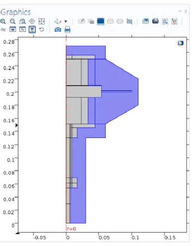
(27) Figure 8: Interior geometry of the model. As the inner gas experiments a heat exchange with the outer fluid, in this case air, the outer fluid needs to be taken into account in the model. Hence, more geometry elements are added to represent the air surrounding the system. These elements are created using the option ‘Polygon’. This air domain is an auxiliary one, which means that its size is not important as long as there is enough space for the fluid properties to develop. It is built around the outer boundaries of the experiment and covers both the lower part that remains still and the upper part, which is in contact with the volume modulation unit – the moving part of the setup.. 18.
(28) Figure 9: Complete previous geometry of the model. Once all the geometry elements have been designed, the last step is to select the option ‘Form Union’ in the ‘Geometry’ menu. It joins all the parts, so that more interfaces and simulation settings can be applied to them.. As it was commented before, the current model does not have the bellows represented like that anymore. A simplification was made to test if there were significant differences regarding the temperature and heat transfer evolution, as that area is where the main heat transfer takes place. In order to do so, instead of the detailed representation of the bellows, just a vertical line indicates the separation between the inner and outer gases. This is possible because, even though the bellows are represented in the previous model geometry, those geometrical elements do not have a physical meaning representing a material part, but just have the function to represent the separation of the fluids. To study the heat transfer with more detail, four new rectangles are created using the ‘Rectangle’ option and placed in the space formerly occupied by the bellows, so that the area remains the same.. 19.
(29) Having two rectangles at each side of the border where the main heat transfer occurs, a finer mesh can be applied in all of them, and thus have more precise results on this area.. Figure 10: Detail of the new geometry. Figure 11: Complete current geometry of the model. 20.
(30) It was confirmed that the temperature evolution does not present significant changes, and reaches its peak at the same time, and physical point, using the simplified geometry, as using the former one. Furthermore, it could be seen that the pressure evolution does not suffer changes because of this modification. Not only does this new geometry allow a finer mesh for the study, but also reduces the simulation time considerably. Due to this reason, this is the geometry which is used from now on to work on the simulation.. 21.
(31) 8 Materials The ‘Materials’ node in COMSOL Multiphysics allows to add predefined or user-defined materials, to specify material properties using model inputs, functions, values, and expressions as needed.. Figure 12: ‘Add Material’ window. The materials for each domain of the model, as well as their properties, need to be defined in order for the software to run the simulation and calculate the different variables which take part in the process. In this model, five materials are defined: The inner fluid of the experiment is Carbon dioxide. It can be selected by right clicking on the ‘Materials’ node and selecting ‘Add Material’. The ‘Add Material’ window is now open and Carbon Dioxide can be found under ‘Liquids and gases’ > ‘Gases’ > ‘Carbon dioxide’. Another possible gas to be used as the inner fluid is Nitrogen. In this case, Nitrogen would be selected following the same procedure as to select the Carbon Dioxide. This change in COMSOL Multiphysics is very easily made, and the inner fluid can be thus changed at any time if necessary. The domains corresponding to the inner fluid (Carbon dioxide) are the following:. 22.
(32) Figure 13: Carbon dioxide domains. The outer fluid is air. It can be found under ‘Add Material’>‘Liquids and gases’ > ‘Gases’ > ‘Air’. Its corresponding domains are the following:. Figure 14: Air domains. 23.
(33) The solid parts of the experiment, like the pipes or rings, are made of steel. The selected material for these domains is steel AISI 4340, found under ‘Add Material’ > ‘Liquids and gases’ > ‘Build in’ > ‘Steel AISI 4340’:. Figure 15: Steel AISI 4340 domains. The reactor wall is made of glass. It can be found under ‘Add Material’ > ‘Liquids and gases’ > ‘Build in’ > ‘Glass (quartz)’.. Figure 16: Glass domain. 24.
(34) Finally, the last material to be added is the Zeolite 5A, the porous material. It cannot be found in COMSOL’s Materials Library, so in this case the steps to follow are right clicking on ‘Geometry’ and selecting ‘Blank Material’. This option allows the user to define the properties for the new material as needed. In this case, the properties that the applied interfaces need, as well as the density and porosity of the zeolite, are manually introduced, either taken from experimental data, or from bibliography [12].. Figure 17: Material Contents table for the Zeolite 5A. This option will facilitate the selection and use of the zeolite properties when applying several interfaces. The domain corresponding to the porous material can be seen in the following image:. Figure 18: Zeolite 5A domain. 25.
(35) 9 Interfaces To incorporate the different interfaces, which COMSOL Multiphysics offers, the ‘Add Physics’ window is used. It can be opened by right clicking on ‘Component’ in the Model Builder tree and then clicking on ‘Add Physics’. Another possibility is to click directly on ‘Add Physics’ in the ‘Physics’ section of the main toolbar. The different interfaces are organized according to their scientific field.. Figure 19: ‘Add Physics’ window. The interfaces used in this model to simulate the real experiment are discussed next. These interfaces are: Laminar Flow, Moving Mesh, Heat Transfer in Solids, and Transport of Diluted Species in Porous Media.. 9.1 Laminar Flow 1 The function of the Laminar Flow (spf) interface is to compute the velocity and pressure fields for the flow of a single-phase fluid in the laminar flow regime. This interface is used twice in this model. In this first case, it is used to compute the pressure and velocity fields of the inner fluid. As it was commented in chapter 3, the laminar Flow interface solves the Navier-Stokes equations for conservation of mass (Eq. 1) and conservation of momentum (Eq. 6) [13]. This interface can be found in the ‘Add Physics window’ under ‘Fluid Flow’ > ‘Single-Phase Flow’ > ‘Laminar Flow (spf)’. It is applied to all the domains corresponding to the inner fluid, in this case, Carbon Dioxide. 26.
(36) Figure 20: Laminar Flow 1 domains. When the ‘Laminar Flow’ interface is added, the following nodes appear by default in the Model Builder: Fluid Properties, Wall (whose default boundary condition is ‘No slip’), Initial Values, and Axial Symmetry. In the ‘Laminar Flow’ settings, the option ‘Compressible Flow (Ma<0.3)’ is selected, and the reference values for temperature and pressure are introduced. Although initially COMSOL expects certain units, it is possible to introduce a numeric value in a different unit, as long as the used unit is specified using square brackets:. Figure 21: Laminar Flow 1 reference values. In the ‘Fluid Properties’ settings, the model inputs are introduced as ‘User defined’. The temperature corresponds to the initial temperature of the experiment, 298.15 K. The absolute pressure, 𝑝𝐴 is expressed by adding 1 atm to the gauge pressure obtained by the simulation, root.comp1.p. The fluid properties, such as density or dynamic viscosity, are selected to be obtained ‘From material’, which means using the properties of the material defined in the corresponding domains.. 27.
(37) Figure 22: Laminar Flow 1 model inputs and fluid properties. For the ‘Initial values’ settings, the velocity field is set up as 0, as there is no movement until the experiment starts. The initial pressure is introduced as gauge pressure, P_N2-Pamb. The initial absolute pressure of the inner gas was parameterized as P_N2, as the inner fluid of the experiment was originally nitrogen, but this initial pressure has the same value when using carbon dioxide, so the defined parameter can be used in the same way without being changed. The ‘Wall’ node permits to add several boundary conditions to describe the fluid-flow behavior. The default boundary condition is ‘No slip’, which prescribes 𝐮 = 0, meaning that the fluid is not moving at the wall. This condition applies to the separation between the inner and outer fluid – the bellows in the real experiment – as well as to the limits of the inner fluid with the not moving materials.. Figure 23: ‘No Slip Wall’ boundaries. 28.
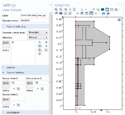
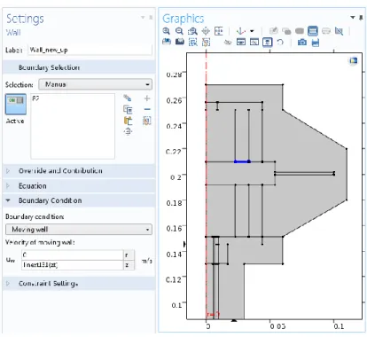
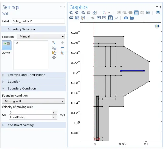
(38) The other boundary condition used is ‘Moving wall’, applied to the boundaries corresponding to the surface of the travel plate in contact with the inner fluid. This boundary condition permits to assign a velocity to the moving wall. The recreation of the movement of the travel plate, by using another interface – Moving Mesh –, will be further described in this chapter. In order to assign a velocity to these boundaries affected by the ‘Moving wall’ condition, and to represent the movement of the fluid in contact with them, it is necessary to create first ‘Linear Extrusion’ coupling operators. They can be created by right clicking on ‘Definitions’ and then selecting ‘Component Couplings’ > ‘Linear Extrusion’. One Linear Extrusion needs to be created for every boundary belonging to the volume-modulation unit representing the separation between each fluid and the solid materials. Both the boundary and its two vertexes need to be selected for each coupling.. Figure 24: Example of the settings of a Linear Extrusion. Once the Linear Extrusions are created, and back in the ‘Laminar Flow’ interface, the velocity of the travel plate can be coupled with the fluid in contact with it. To achieve this, the z axis velocity needs to be introduced for the boundaries of the travel plate with ‘Moving wall’ condition. For each of them, the velocity will be their corresponding ‘Linear extrusion’ – written as the shortcut linext – followed by ‘(zt)’ to indicate that the complete expression is a velocity:. 29.
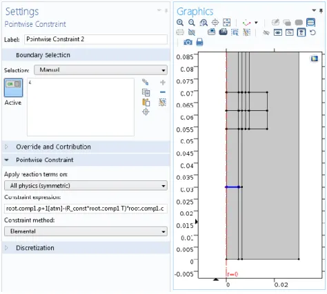
(39) Figure 25: Example of the settings of a ‘Moving Wall’ in Laminar Flow 1. Finally, the last main node used in this interface is a ‘Pointwise Constraint’. The steps to select it consist of clicking in ‘Show’ at the top of the Model Builder tree and then on ‘Advanced Physic Options’. This permits to find the ‘Pointwise Constraint’ by right clicking on ‘Laminar Flow’ and then selecting ‘Points’ > ‘Pointwise Constraint’. The ‘Pointwise Constraint’ is applied on the boundary which represents the separation between the inner fluid and the porous material, in the reactor. As it will be discussed later in this chapter, the variation of the pressure, as a result of the inner gas being compressed and expanded, favors the adsorption and desorption of the inner fluid in the porous material. As a consequence, the variation of the concentration of the inner fluid in the porous material has also an influence in the pressure of the inner gas: When the porous material adsorbs gas, the pressure in the reactor decreases, whereas when desorption occurs, the pressure in the reactor increases. In order to recreate this relation in the model, the Ideal Gas law is used to express the inner gas pressure as a function of the gas concentration in the porous material:. 𝑃=. 𝑛 𝑅𝑇=𝑐𝑅𝑇 𝑉. (Eq. 21). The ‘Pointwise Constraint’ sets equal to zero the introduced constraint expression. Therefore, to introduce as a condition that the pressure at the boundary separating the fluid and the porous material suffers a change due to the variation of concentration, the pressure of the inner fluid minus the pressure expressed as a function of the concentration is written as the constraint expression – this is the same as equalizing both expressions of the pressure, establishing that the pressure at that boundary will depend on the concentration changes. 30.
(40) In terms of the model variables, this constraint expression is written as: 𝑟𝑜𝑜𝑡. 𝑐𝑜𝑚𝑝1. 𝑝 + 1[𝑎𝑡𝑚] − (𝑅_𝑐𝑜𝑛𝑠𝑡 ∗ 𝑟𝑜𝑜𝑡. 𝑐𝑜𝑚𝑝1. 𝑇) ∗ 𝑟𝑜𝑜𝑡. 𝑐𝑜𝑚𝑝1. 𝑐. Figure 26: Settings and selected boundary of the ‘Pointwise Constraint’. Being 𝑟𝑜𝑜𝑡. 𝑐𝑜𝑚𝑝1. 𝑝 + 1[𝑎𝑡𝑚] the expression of the pressure of the inner fluid with which the program works, and (𝑅_𝑐𝑜𝑛𝑠𝑡 ∗ 𝑟𝑜𝑜𝑡. 𝑐𝑜𝑚𝑝1. 𝑇) ∗ 𝑟𝑜𝑜𝑡. 𝑐𝑜𝑚𝑝1. 𝑐 the pressure expressed as a function of the concentration variation of the gas in the porous material.. 9.2 Laminar Flow 2 A second ‘Laminar Flow’ interface is applied to the outer fluid to calculate its velocity and pressure fields during the experiment. In this case, the outer fluid is the air of the environment. The second ‘Laminar Flow’ is then applied to every domain corresponding to air:. 31.
(41) Figure 27: ‘Laminar Flow 2’ domains. The reference values and ‘Compressible Flow’ option are the same as for the inner fluid. The model inputs are also introduced in the same way, and the fluid properties are taken ‘From material’.. Figure 28: Laminar Flow 2 model inputs and fluid properties. 32.
(42) The ‘No Slip Wall’ boundary condition which appears by default has the same effect as in the previous ‘Laminar Flow’ interface, but this time form the other side. Likewise, to match the movement of the travel plate and its effect on the air, the ‘Moving Wall’ nodes are needed. The steps to couple the ‘Laminar Extrusion’ functions created under ‘Definitions’ with the ‘Moving Wall’ nodes are the same as in the first ‘Laminar Flow’ interface. The expression of velocity in the z axis is also the shortcut for the corresponding Laminar Extrusion followed by (zt):. Figure 29: Example of the settings of a ‘Moving Wall’ in Laminar Flow 2. Another boundary condition used in this interface is ‘Open Boundary’, which can be found by right clicking on ‘Fluid Flow 2’. The ‘Open Boundary’ condition describes boundaries in contact with a large volume of fluid, in this case, the air of the environment surrounding the experiment. Fluid can both enter and leave the domain on boundaries with this type of condition.. 33.
(43) All the outer boundaries of the outer fluid are selected. The boundary condition is selected as ‘Normal stress’ with a value of 0 N/m2 .. Figure 30: Settings and selected boundaries of ‘Open Boundary’ in Laminar Flow 2. 9.3 Moving Mesh The Moving Mesh (ale) interface can be used to create models where the geometry experiments shape changes provoked by physical phenomena without material being removed or added. When using this interface, the changing geometry is represented by the mesh. The Moving Mesh interface can be found in the ‘Add Physics’ window under ‘Mathematics’ > ‘Deformed Mesh’ > ‘Moving Mesh’. There is another interface under the same branch, called ‘Deformed Geometry’. This other interface is not used, as it defines a deformation of the material frame relative to the geometry frame, rather than a displacement of the spatial frame relative to the material frame. The second option is what can be applied to simulate the experiment, and it is what ‘Moving Mesh’ defines [14].. 34.
(44) The selected domains for the ‘Moving Mesh’ interface are those which represent the moving part of the model, in other words, the domains corresponding to the volume-modulation unit: The travel plate, and the domains of inner and outer fluids which are affected – compressed and expanded – by this movement in the top part:. Figure 31: ‘Moving Mesh’ domains. The default nodes which are added to the Model Builder together with the ‘Moving Mesh’ interface are: Fixed Mesh, and Prescribed Mesh Displacement. In order to add more nodes representing the different conditions, it is necessary to right click on ‘Moving Mesh’ and then select ‘Free Deformation’. The Free Deformation node constrains the mesh displacement only by the boundary conditions on the surrounding boundaries. The initial mesh displacement can be introduced, which in this case is 0 m both in the z and r directions, since there is no movement until the experiment begins. The selected domains are the same as for the ‘Moving Mesh’ interface – the moving parts. Finally, by right clicking again in ‘Moving Mesh’, the node ‘Prescribed Mesh Displacement’ can be selected. This node is used three times in this model. The ‘Prescribed Mesh Displacement’ node permits to specify the displacement of the boundaries of domains with free deformation. The spatial frame in the adjacent domain moves in accordance with the displacement.. 35.
(45) The first ‘Prescribed Mesh Displacement’ is used to represent the vertical movement of the travel plate, which is what causes the volume modulation. In order to achieve this, the wave function created in ‘Definitions’ is used. The selected boundaries are the ones representing the travel plate. The travel plate only moves in the z axis, so the prescribed z displacement is set as wave(t[1/s]) m, which means that the z displacement will behave over time following the periodic function. As the units of the displacement must be length units, the [1/s] is multiplied to the expression of time [s].. Figure 32: Settings and selected boundaries of Prescribed Mesh Displacement 1. The second ‘Prescribed Mesh Displacement’ is applied to the boundaries belonging to the symmetry axis and its function is to restrict the horizontal movement of these boundaries, having 0 m as the value of the prescribed r displacement.. 36.
(46) Figure 33: Settings and selected boundaries of Prescribed Mesh Displacement 2. To conclude, the third and last ‘Prescribed Mesh Displacement’ is applied to the outer boundaries of the volume-modulation unit to indicate that these boundaries do not have any movement. Both prescribed r and z displacements are selected as 0 m.. Figure 34: Settings and selected boundaries of Prescribed Mesh Displacement 3. 37.
(47) 9.4 Heat Transfer in Solids The Heat Transfer in Solids (ht) interface can be used to model heat transfer in solids by conduction, convection, and radiation. It can be found in the ‘Add Physics’ window under ‘Heat Transfer’ > ‘Heat Transfer in Solids’. The name of the interface is ‘Heat Transfer in Solids’, however, it can also be applied to fluids using specific nodes. The equation that this interface solves is the differential form of the Fourier’s Law (Eq. 7), and it is possible to add heat sources to represent additional contributions. The default nodes which are added to the Model Builder when ‘Heat Transfer in Solids’ is incorporated are: Solid, Thermal Insulation (the default boundary condition), Initial Values, and Axial Symmetry. Then, by right clicking on the node in the Model Builder tree or directly from the ‘Physics’ toolbar, other nodes to implement physic features, boundary conditions or heat sources can be added [15].. All the domains are selected for the ‘Heat Transfer in Solids’ interface, and the ambient temperature and ambient pressure are introduced as 293.15 K and 1 atm, respectively. The temperature at the ‘Initial Values’ node is introduced as ‘User defined’, using the already defined parameter T_amb. Then, for the ‘Solid’ node – which is renamed as ‘Heat Transfer in Solids’ – the domains corresponding to the glass reactor, the steel parts, and the porous material are selected. The absolute pressure is set as 1 atm, and the option ‘From material’ is chosen for the program to obtain the properties such as thermal conductivity, density and heat capacity at constant pressure from the information of the material defined in each of the selected domains.. Figure 35: ‘Solid’ node domains. 38.
(48) The ‘Thermal Insulation’ node indicates that there is no heat flux across the selected boundary, 𝐧 ∙ 𝐪 = 0, and hence, establishes where the domain is insulated. The ‘Thermal Insulation’ node is applied at the left bottom boundary of the model, to insulate the reactor, where the porous material is placed.. Figure 36: ‘Thermal Insulation’ boundary. For the rest of the boundaries, the node ‘Open Boundary’ is used. It works in the same way as in the ‘Laminar Flow’ interface, except that in this case the boundary condition is established as temperature, being T_amb the parameter introduced.. Figure 37: Settings and selected boundaries of ‘Open Boundary’ in Heat Transfer. 39.
(49) In order to simulate the heat transfer in fluids, another node is selected by right clicking on ‘Heat Transfer in Solids’ and then selecting ‘Fluid’. This node is used twice – one time for each fluid – and renamed as ‘Heat Transfer in Fluids 1’ and ‘Heat Transfer in Fluids 2’. For ‘Heat Transfer in Fluids 1’, the domains corresponding to the inner gas are selected. The absolute pressure is defined as root.comp1.p+1[atm] and the velocity field is coupled with the ‘Laminar Flow 1’ node by selecting ‘Velocity field (spf)’. The fluid properties used by the interface are introduced as ‘From material’ so that the program takes the properties values form the material defined in those domains. As it was commented in chapter 3, all the generated heat appears as a consequence of the movement of the fluid, so the two terms representing the heat origin are: The work done by changes of pressure which affects the temperature of the fluid (Eq. 9), and the viscous dissipation in the fluid (Eq. 10). To incorporate these effects to the model, the nodes ‘Pressure Work’ and ‘Viscous Heating’ are selected respectively. They can be found by right clicking on ‘Heat Transfer in Fluids 1’. The absolute pressure in the ‘Viscous Heating’ settings is also introduced as root.comp1.p+1[atm], and the dynamic viscosity is taken ‘From material’.. For ‘Heat Transfer in Fluids 2’, the domains corresponding to the outer gas are selected. The steps to follow are the same as for the ‘Heat Transfer in Fluids 1’ node. The absolute pressure in this case is introduced as 1[atm], which is the ambient pressure, and the properties are also taken ‘From material’. The nodes ‘Pressure Work’ and ‘Viscous Heating’ are also applied here, being the absolute pressure in the ‘viscous Heating’ settings expressed as root.comp1.p2+1[atm].. Finally, the node ‘Thin Thermally Resistive Layer’ is selected under ‘Heat Transfer in Solids’, to be applied in the boundaries where the inner and outer fluids are in contact. There is a line indicating the separation of the fluids where the bellows are placed in the real experiment. This permits to divide the space in several domains, but it is not enough to represent the resistive material between the fluids. This ‘Thin Thermally Resistive Layer’ is applied to complete it by introducing the thickness and thermal conductivity of this material, which are defined as 0.2 mm and 16 W/(mK) respectively [16].. 40.
(50) Figure 38: ‘Thin Thermally Resistive Layer’ boundaries. 9.5 Transport of Diluted Species in Porous Media The Transport of Diluted Species in Porous Media (tds) interface is used to simulate the mass transport in the porous material. The function of this interface is to calculate the species concentration and transport in free and porous media. It is the same interface as Transport of Diluted Species but presents other default nodes, such as the ‘Porous Media Transport Properties’ node. The rest of the default nodes that appear when the ‘Transport of Diluted Species in Porous Media’ interface is selected are: Axial Symmetry, No Flux, and Initial Values. More nodes can be added by right clicking on the interface in the Model Builder tree. The ‘Transport of Diluted Species in Porous Media’ interface can simulate free and porous media flow with immobile and mobile phases, and supports several processes such as diffusion, convection, dispersion, adsorption, and volatilization in porous media. It can be applied to cases in which the solid phase substrate is immobile, as well as to cases in which a gas-filling medium is also assumed to be immobile. The mass transport which can be defined with this interface can be applied to one or more diluted species or solutes which move within a fluid that fills (saturated) or partially fills (unsaturated) the voids in a solid porous medium. When the pore space is not filled with fluid, then the pore space contains an immobile gas phase [17]. 41.
(51) The domain in which this interface is applied is the domain corresponding to the porous material. Diffusion is included in the study, but to include also the adsorption and desorption processes, the option ‘Adsorption in porous media’ needs to be selected in the ‘Additional transport mechanisms’.. Figure 39: ‘Transport of Diluted Species’ domain. Figure 40: Selection of ‘Adsorption’ in the Transport Mechanisms section. The main node of the ‘Transport of Diluted Species in Porous Media’ interface is ‘Porous Media Transport Properties’. In the Settings of this node, the model inputs are defined. The velocity field is introduced as 0, as the porous material is an immobile solid, and the absolute pressure is coupled with the ‘Laminar Flow 1’ interface by selecting ‘Absolute pressure (spf)’. 42.
(52) In the ‘Matrix Properties’ section of the settings, for the Porous material the selected option is ‘Domain material’, as the porous solid – the Zeolite 5A – was already defined in that domain. The properties such as density and porosity are obtained using the ‘From material’ option, once the material has been specified.. Figure 41: ‘Matrix properties’ settings. In the ‘Diffusion’ section, carbon dioxide is selected as the fluid material, and the experimental data such as the fluid diffusion coefficient 𝐷𝐹,𝑐 is introduced as 5 ∙ 10−5 m2 /s.. Figure 42: ‘Diffusion’ settings. 43.
(53) In the ‘Adsorption’ section of the settings, the Langmuir sorption type is used, and the Langmuir constant 𝐾𝐿,𝑐 and the adsorption maximum 𝑐𝑃,𝑚𝑎𝑥,𝑐 are given the values of 1.5 m3 /mol, and 4.5 mol/kg, respectively.. Figure 43: ‘Adsorption’ settings. In the ‘Initial Values’ node, the value for the initial concentration of the fluid in the porous material needs to be introduced. The Ideal Gas law (Eq. 21) is used to calculate the initial concentration, based on the initial pressure and the initial temperature of the reactor:. 𝑐0 =. 𝑃𝑜 𝑅 ∙ 𝑇0. (Eq. 22). Thus, being the initial absolute pressure 𝑃𝑜 = 133 Pa, and the initial temperature 𝑇0 = 298.15 K, the initial gas concentration in the porous material is set to be 𝑐0 = 0.054 mol/m3.. Finally, to express the gas flowing into the reactor and its contact with the porous material, the ‘No Flux’ and ‘Inflow’ nodes are used. The ‘No Flux’ node is the default boundary condition on exterior boundaries. It represents boundaries where there is no mass flow in or out of the selected boundaries. Hence, the total flux in these boundaries is zero. This node is used to indicate that the gas only flows in the reactor from the top part, as the rest of the reactor – sides and bottom – is closed. This can be expressed in the model by applying the ‘No Flux’ node to the right and bottom boundaries of the domain corresponding to the porous material.. 44.
Figure
![Figure 1: Fundamental concept of frequency response analysis. Taken from [4].](https://thumb-us.123doks.com/thumbv2/123dok_es/2877845.548608/17.918.207.713.408.770/figure-fundamental-concept-frequency-response-analysis-taken.webp)
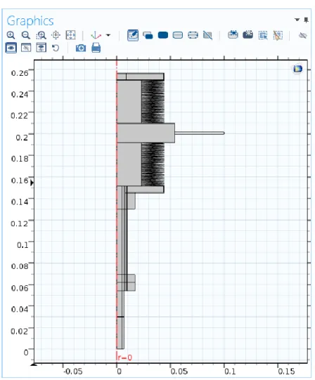
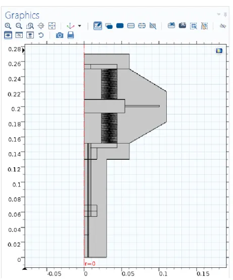
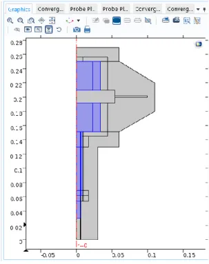
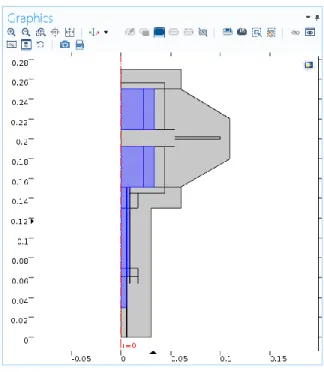
+7
Documento similar
Los objetivos principales que se querían lograr en este trabajo eran tres: el primero era desarrollar un modelo de Dinámica de Fluidos Computacional (CFD) para
MD simulations in this and previous work has allowed us to propose a relation between the nature of the interactions at the interface and the observed properties of nanofluids:
It could maybe seem somehow insubstantial to consider an actual increase in computing power produced merely by a change in representation, consid- ering that computable functions
The RT system includes the following components: the steady state detector used for model updating, the steady state process model and its associated performance model, the solver
In the previous sections we have shown how astronomical alignments and solar hierophanies – with a common interest in the solstices − were substantiated in the
Instrument Stability is a Key Challenge to measuring the Largest Angular Scales. White noise of photon limited detector
It might seem at first that the action for General Relativity (1.2) is rather arbitrary, considering the enormous freedom available in the construction of geometric scalars. How-
teriza por dos factores, que vienen a determinar la especial responsabilidad que incumbe al Tribunal de Justicia en esta materia: de un lado, la inexistencia, en el
