Characterization of arc extinction in direct current residential circuit breakers

Texto completo

(1)Instituto Tecnológico y de Estudios Superiores de Monterrey Campus Monterrey. School of Engineering and Sciences. Characterization of Arc Extinction in Direct Current Residential Circuit Breakers A thesis presented by. Julio César Bautista Cruz Submitted to the School of Engineering and Sciences in partial fulfillment of the requirements for the degree of. Master of Science In Energy Engineering. Monterrey Nuevo León. May 15th, 2018.

(2)

(3) Instituto Tecnológico y de Estudios Superiores de Monterrey Campus Monterrey School of Engineering and Sciences The committee members, hereby, certify that have read the thesis presented by Julio César Bautista Cruz and that it is fully adequate in scope and quality as a partial requirement for the degree of Master of Science in Energy Engineering.. Thesis Committee:. ____________________________________ Federico Ángel Viramontes Brown, PhD Tecnológico de Monterrey Principal Advisor. ____________________________________ Carlos Iván Rivera Solorio, PhD Tecnológico de Monterrey Committee Member. ____________________________________ José Carlos Suarez Guevara, M.SC Schneider-Electric Committee Member. ____________________________________ Efrain Gutierrez Villanueva, M.SC Schneider-Electric Committee Member. _____________________________________ Ruben Morales Melendez, PhD Dean of Graduate Studies School of Engineering and Sciences Monterrey Nuevo León. May 15th, 2018.

(4)

(5) Declaration of Authorship I, Julio César Bautista Cruz, declare that this thesis titled, “Characterization of Arc Extinction in Direct Current Residential Circuit Breakers” and the work presented in it are my own. I confirm that:     . This work was done wholly while in candidature for the degree of Master of Science at this University. Where I have consulted the published work of others, this is always clearly attributed. Where I have quoted from the work of others, the source is always given. With the exception of such quotations, this thesis is entirely my own work. I have acknowledged all main sources of help. I have given credence to the contributions of the co-authors.. ___________________________ Julio César Bautista Cruz Monterrey Nuevo León, May 2018. @2018 by Julio César Bautista Cruz All rights reserved.

(6)

(7) Dedication To Yahveh my Lord, who has given me the life and has allowed me to consummate my master's degree, providing me the cleverness, talent, resources and especially wonderful people who motivated me to move forward..

(8)

(9) Acknowledgment To Osvaldo Micheloud and Federico Viramontes for calling me to be part of the Industrial Consortium to Foster Applied Research in Mexico and for allowing me to join this great research group.. To my advisor Federico Viramontes, for his support and advice at each stage of the project, his constant motivation despite all the obstacles encountered and mainly by all the classes taught by him, always interesting, challenging and with a well-founded purpose.. To Carlos Rivera, for his advice, suggestions, collaboration on this project, and for the careful revision of the manuscript and useful discussion.. To Efraín Gutiérrez, Mauricio Diaz, José Suarez, José Valerio, of Schneider-Electric, for supporting me in different means, in addition to the resources for carrying out this research, review of the manuscript and constant motivation.. To all my professors, since each one of their teaching were vital during the development of this research..

(10)

(11) Everything I have accomplished, beyond my effort, has been the result of my patience. Julio Bautista.

(12)

(13)

(14)

(15) Contents Abstract. ................................................................................................................................... i Resumen ................................................................................................................................ iii List of Figures ......................................................................................................................... v List of Tables ......................................................................................................................... ix Lexicon .................................................................................................................................. xi 1.. 2.. CHAPTER I.................................................................................................................... 1 1.1.. Introduction .............................................................................................................. 1. 1.2.. Problem Statement ................................................................................................... 2. 1.3.. Objectives ................................................................................................................ 2. 1.4.. Justification .............................................................................................................. 2. 1.5.. Research questions ................................................................................................... 3. 1.6.. Scope and Limitations ............................................................................................. 3. 1.7.. Thesis structure ........................................................................................................ 3. CHAPTER II .................................................................................................................. 5 2.1.. Characteristics of the electric arc ............................................................................. 5. 2.2.. Low voltage circuit breakers .................................................................................... 7. Interruption in LVCB ..................................................................................................... 7 2.3.. The Limiter Circuit Breaker .................................................................................... 9. 2.3.1 Arc breaking .......................................................................................................... 9 2.3.2 Kind of breaking in established currents ............................................................. 10 2.3.3 Arc breaking with limitation................................................................................ 11 2.4.. Consequences of Arcing ........................................................................................ 11. 2.4.1 Contact Erosion ................................................................................................... 11 2.5.. Components of CB................................................................................................. 12. 2.5.1 Frame ................................................................................................................... 12 2.5.2 Contacts ............................................................................................................... 13 2.5.3 Arc Chute Assembly............................................................................................ 13 2.5.4 Operating Mechanism ......................................................................................... 14 2.5.5 Trip Unit .............................................................................................................. 14.

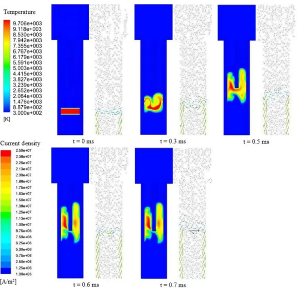
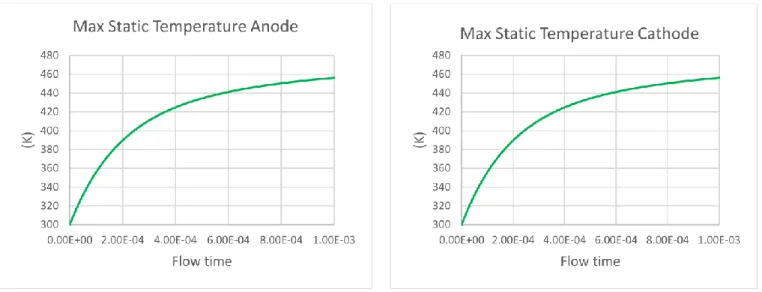
(16) 2.6.. Arc manipulation ................................................................................................... 15. 2.6.1. Open Gap ............................................................................................................ 15 2.6.2. Arc Runner ......................................................................................................... 15 2.6.3. Blowout Coils ..................................................................................................... 16 2.6.4. Puffer .................................................................................................................. 16 2.7.. Theory of Multi-physical Fields in a Fault Arc ..................................................... 17. 2.8.. Fluid Models Magnetohydrodynamic description ................................................. 19. 2.9.. Simulation tool. ...................................................................................................... 20. 2.9.1 Ansys-Fluent. ....................................................................................................... 20 2.9.2 ANSYS-Maxwell. ............................................................................................... 21 2.9.3 Altair-Flux ........................................................................................................... 22 3.. Chapter III..................................................................................................................... 25 3.1.. Methodology for simulation .................................................................................. 25. 3.2.. Description model .................................................................................................. 27. 3.2.1 Geometry model .................................................................................................. 27 3.2.2 Mesh .................................................................................................................... 27 3.2.3 Plasma properties as UDF ................................................................................... 30 3.2.4 Interfaces and boundary conditions ..................................................................... 33 3.2.5 Parametrization .................................................................................................... 35 3.3.. Software Set-up ...................................................................................................... 35. 3.3.1 Set up in MHD module........................................................................................ 35 4.. 5.. Chapter IV .................................................................................................................... 45 4.1.. Simulations cases ................................................................................................... 45. 4.2.. Case A: Justification analysis ................................................................................ 46. 4.3.. Case B: Base Model ............................................................................................... 47. 4.4.. Case C: Coupling Maxwell-Fluent ........................................................................ 47. 4.5.. Case D: Coupling Flux-Fluent ............................................................................... 48. 4.6.. Case E: Comparative analysis ................................................................................ 48. Chapter V...................................................................................................................... 49 5.1.. Case A1. Justification analysis (3DS model) ......................................................... 49. 5.2.. Case A2. Justification analysis (3DF model) ......................................................... 51. Comparison case A1 vs case A2 .................................................................................. 52.

(17) 5.3.. Case B1. Base Model (laminar regimen) ............................................................... 53. 5.4.. Case B2. Base Model (turbulent regimen) ............................................................. 60. Comparison case B1 vs case B2 ................................................................................... 67 5.5.. Case C1. Coupling Maxwell-Fluent ...................................................................... 68. 5.6.. Case D1. Coupling Flux-Fluent ............................................................................. 72. Comparison case C1 vs case D2 ................................................................................... 73 5.7.. Case E1. Comparative analysis .............................................................................. 74. Comparison case B2 vs case E1 ................................................................................... 79 6.. Chapter VI .................................................................................................................... 81. 7.. Chapter VII ................................................................................................................... 85. Bibliography ......................................................................................................................... 87 A.. Appendix A. The Physics of Electric Arc. ................................................................... 91. B.. Appendix B. The MHD module of Ansys-Fluent. ....................................................... 93. C.. Appendix C. User Define Functions (UDFs) ............................................................... 97. D.. Annex D...................................................................................................................... 101. E.. Annex E ...................................................................................................................... 107. Vita ..................................................................................................................................... 109.

(18)

(19) Characterization of Arc Extinction in Direct Current Residential Circuit Breakers By Julio César Bautista Cruz. Abstract. Break the current in a direct current (DC) network is a challenging theme, since the current does not exhibit a zero crossing point, making it difficult to interrupt. Recent researches show promising results in the development of Circuit Breakers (CB) for DC, with different configurations to achieve an artificial zero crossing. However, regardless of the method, the physical effect of switching is the formation of an electric arc, causing high levels of temperature, strong magnetic fields, current of several tens of KA, added to mechanical stress and overpressure on the walls. Due to this reason, physical phenomena should be studied to determine a suitable design. This thesis aim is to provide a methodology for the modeling and the comprehension of the physics that governs electric arc and the role of each component within the CB. To reach this, the thesis starts by understanding the arc in alternating current (AC), then proceeds to DC. A theoretical description of the electric arc is outlined, based on plasma physics. The Magneto-Hydrodynamic (MHD) model is proposed, which allows modeling a plasma as an electric fluid, allowing coupling the equations of fluid mechanics and magnetic fields. The scope of the model is the macroscopic scale of the arc dynamics as a conducting, compressible, viscid fluid, driven by electromagnetic forces and pressure gradients. Some analysis are performed in different software and a comparative analysis is accomplished. Finally, the aim of this thesis is to provide to Schneider-Electric Company the background for this kind of analysis in DC CB.. i.

(20) ii.

(21) Resumen Interrumpir el voltaje en una red de corriente directa (DC) es un tema retador, debido a que la corriente no exhibe un cruce por cero natural, lo que dificulta la interrupción. Investigaciones recientes muestran resultados prometedores en el desarrollo de Circuit Breakers (CB) para CD, con diferentes configuraciones para lograr un cruce por cero artificial. Sin embargo, independientemente del método que se use, el efecto de la interrupción es la formación de un arco eléctrico, causando incrementos de temperatura, fuertes campos magnéticos, corrientes de varias decenas de KA, sumado a los esfuerzos mecánicos provocados por la presión en las paredes. Por estas razones, estos fenómenos físicos deben estudiarse para determinar un diseño adecuado. Esta tesis tiene como finalidad proporcionar una metodología para el modelado y la comprensión de la física que rige el fenómeno de arco eléctrico y el papel de cada componente dentro del CB. Para llegar a esto, la tesis comienza explicando el fenómeno en corriente alterna (AC), y luego se procede en CD. Además, se describe la teórica del arco eléctrico basada en la física del plasma. Para esto, se propone el modelo Magneto-hidrodinámico (MHD) en ANSYS-Fluent, que permite modelar un plasma como un fluido eléctrico, permitiendo el acoplamiento de las ecuaciones de la mecánica de fluidos y los campos magnéticos. El alcance del modelo es un análisis macroscópico, viendo al arco como un fluido conductor, compresible y viscoso, impulsado por fuerzas electromagnéticas y gradientes de presión. Algunos análisis se realizan en diferentes programas y se realiza un análisis comparativo entre ellos. Finalmente, el objetivo de esta tesis es proporcionar a la compañía Schneider-Electric las bases para este tipo de estudios en Circuit Brakers de CD.. iii.

(22) iv.

(23) List of Figures Figure 2-1: Cathode fall [16] ............................................................................................................................... 5 Figure 2-2: Anode fall [16] .................................................................................................................................. 6 Figure 2-3 Double break rotary contact, Patent number: 8,159,319 B2. ........................................................... 8 Figure 2-4 the electric arc, composition of the arc column. [28] ........................................................................ 9 Figure 2-5 Arc in extinguishing condition. a- in DC. voltage b- in AC. voltage with Ur of same sign as Ua at the time of zero current [28]. .................................................................................................................................. 10 Figure 2-6 equivalent circuit in a short circuit fault. ......................................................................................... 10 Figure 2-7 Frame of a Circuit Breaker [31]. ...................................................................................................... 12 Figure 2-8 Straight through contacts and bow apart contacts [30]. ................................................................ 13 Figure 2-9 Arc chute assembly [30]. ................................................................................................................. 14 Figure 2-10 Operating mechanism, a) ON position, b) OFF position [30]. ........................................................ 14 Figure 2-11 Thermal-Magnetic trip unit [30]. ................................................................................................... 15 Figure 2-12 Assembling of arc runners [32]. ..................................................................................................... 16 Figure 2-13 Blowout coils assembling [34]. ...................................................................................................... 16 Figure 2-14 Puffer type SF6 CB, a) ON position, b) OFF position [35]. .............................................................. 17 Figure 2-15 Interaction of physical processes in the arc column [9]. ................................................................ 23 Figure 3-1 Toolbox of Fluent. ............................................................................................................................ 25 Figure 3-2 Geometry with dimensions. ............................................................................................................. 27 Figure 3-3 Overview of the full mesh (a), detailed (b). ..................................................................................... 29 Figure 3-4 Skewness of 3DF mesh. .................................................................................................................... 29 Figure 3-5 Orthogonal quality of 3DF mesh. ..................................................................................................... 29 Figure 3-6 Skewness of 3DS mesh. .................................................................................................................... 30 Figure 3-7 Orthogonal quality of 3DS mesh. ..................................................................................................... 30 Figure 3-8 Density for high temperature air [42], a) plot in TI-Nspire CX CAS software, b) plot in Excel. ........ 31 Figure 3-9 Specific Heat for high temperature air [42], a) plot in TI Nspire CX CAS software, b) plot in Excel. 31 Figure 3-10 Thermal Conductivity for high temperature air [42], a) plot in TI-Nspire CX CAS software, b) plot in Excel. ............................................................................................................................................................. 31 Figure 3-11 Viscosity for high temperature air [42], a) plot in TI-Nspire CX CAS software, b) plot in Excel. .... 32 Figure 3-12 Electric Conductivity for high temperature air [42], a) plot in TI-Nspire CX CAS software, b) plot in Excel.................................................................................................................................................................. 32 Figure 3-13 Boundary conditions on the model................................................................................................ 34 Figure 3-14 Modules of ANSYS Fluent. ............................................................................................................. 36 Figure 3-15 Set-up MHD module. ..................................................................................................................... 36 Figure 3-16 Set-up of transient simulation, P1 radiation model and turbulent analysis. ................................. 37 Figure 3-17 Compilation of plasma properties. ................................................................................................ 37 Figure 3-18 Loading material properties. ......................................................................................................... 37 Figure 3-19 Set-up cell zone condition. ............................................................................................................. 37 Figure 3-20 Configuration of limits of the simulation. ...................................................................................... 38 Figure 3-21 Advance configurations for the solution controls. ......................................................................... 38 Figure 3-22 Solution Methods Set-up Fluent. ................................................................................................... 38 Figure 3-23 Solution Controls Set-up Fluent. .................................................................................................... 38 Figure 3-24 Set-up of Run Calculation. ............................................................................................................. 39 Figure 3-25 Toolbox of Maxwell. ...................................................................................................................... 39 Figure 3-26 Assignation of each zone in the geometry .................................................................................... 39 Figure 3-27 Set-up of Magnetostatic simulation and assign of direction current in Maxwell. ......................... 40. v.

(24) Figure 3-28 Set-up Mesh length in Maxwell. .................................................................................................... 40 Figure 3-29 Configuration of Fluent conductivity coupling............................................................................... 41 Figure 3-30 Validation check of the set-up. ...................................................................................................... 41 Figure 3-31 Geometry imported from the modeler context. ............................................................................ 41 Figure 3-32 Mesh model of the CB. .................................................................................................................. 42 Figure 3-33 Configuration of the formulation model in Transient Magnetic 3D application. .......................... 42 Figure 3-34 Current applied to the model in the circuit dedicated context. ..................................................... 42 Figure 3-35 Importing material from material manager. ................................................................................. 43 Figure 3-36 Assignment terminals to solid conductors. .................................................................................... 43 Figure 3-37 Scenario to solve the MCCB extinction module model. ................................................................. 44 Figure 5-1 Arc movement, expressed by temperature for case A1. .................................................................. 50 Figure 5-2 Maximum temperature in air for case A1. ...................................................................................... 50 Figure 5-3 Arc movement, expressed by temperature for case A2. .................................................................. 51 Figure 5-4 Maximum temperature in air for case A2. ...................................................................................... 52 Figure 5-5 Arc movement, expressed by temperature and current density for case B1. .................................. 53 Figure 5-6 Maximum electric potential for case B1. ......................................................................................... 54 Figure 5-7 Maximum temperature in air for case B1. ...................................................................................... 55 Figure 5-8 Maximum temperature in Anode and Cathode for case B1. ........................................................... 56 Figure 5-9 Maximum temperature in splitter for case B1. ............................................................................... 56 Figure 5-10 Maximum radiation temperature for walls for case B1. ............................................................... 57 Figure 5-11 Maximum current density in air for case B1. ................................................................................. 58 Figure 5-12 Maximum current density at the splitter for case B1. ................................................................... 58 Figure 5-13 Maximum absolute pressure for case B1. ..................................................................................... 59 Figure 5-14 Arc movement, expressed by temperature and current density for case B2. ................................ 61 Figure 5-15 Maximum electric potential for case B2. ....................................................................................... 62 Figure 5-16 Maximum temperature in air for case B2. .................................................................................... 63 Figure 5-17 Maximum temperature in Anode and Cathode for case B2. ......................................................... 63 Figure 5-18 Maximum temperature in splitter for case B2. ............................................................................. 64 Figure 5-19 Maximum radiation temperature for walls for case B2. ............................................................... 64 Figure 5-20 Maximum current density in the air for case B2. .......................................................................... 65 Figure 5-21 Maximum current density at the splitter for case B2. ................................................................... 66 Figure 5-22 Maximum absolute pressure for case B2. ..................................................................................... 66 Figure 5-23 Arc movement, expressed by temperature (left) and current density (right) for case C1. ............ 68 Figure 5-24 Maximum temperature in Air for case C1. .................................................................................... 69 Figure 5-25 Arc movement, expressed by Magnetic Flux Density for case C1. ................................................. 70 Figure 5-26 Maximum magnetic flux density for case C1. ................................................................................ 71 Figure 5-27 Arc movement, expressed by geometry for case D1. .................................................................... 72 Figure 5-28 Maximum magnetic flux density for case D1. ............................................................................... 73 Figure 5-29 Arc movement, expressed by temperature and current density for case E1. ................................ 74 Figure 5-30 Maximum temperature in Air for case E1. .................................................................................... 75 Figure 5-31 Maximum temperature in Anode and Cathode for case E1. ......................................................... 76 Figure 5-32 Maximum current density in the air for case E1. ........................................................................... 76 Figure 5-33 Maximum current density at the splitter for case E1. ................................................................... 77 Figure 5-34 Maximum electric potential for case E1. ....................................................................................... 77 Figure 5-35 Maximum radiation temperature for walls for case E1. ............................................................... 78 Figure 5-36 Maximum absolute pressure for case E1. ...................................................................................... 79 Figure A-1 Electron trajectory in a homogeneous electric field. The trajectory is interrupted by elastic collisions with neutral atoms.[45] .................................................................................................................... 92 Figure B-1 Modules of ANSYS Fluent. ............................................................................................................... 95. vi.

(25) Figure C-1 Grid components [41]. ..................................................................................................................... 98 Figure C-2 Example of UDF codification. .......................................................................................................... 99 Figure D-1 Arc movement images from reference [9]. ................................................................................... 101 Figure D-2 Arc movement, (temperature and current density) for case B1. ................................................... 102 Figure D-3 Arc movement, (temperature and current density) for case B2. ................................................... 103 Figure D-4 Arc movement, (temperature and current density) for case C1. ................................................... 104 Figure D-5 Arc movement, (temperature and current density) for case E1. ................................................... 105. vii.

(26) viii.

(27) List of Tables Table 2-1 Minimum voltage and current in different materials ......................................................................... 6 Table 3-1 Description of the 3DF mesh ............................................................................................................. 28 Table 3-2 Description of the 3DS mesh. ............................................................................................................ 28 Table 3-3 Boundary conditions applied in the model ....................................................................................... 33 Table 4-1 Cases analyzed .................................................................................................................................. 45 Table B-1 User-Define Scalars in MHD Model .................................................................................................. 95 Table C-1 Grid nomenclature. ........................................................................................................................... 98. ix.

(28) x.

(29) Lexicon 2D. Bi-dimensional 3D. Tri-dimensional 3DF. Tridimensional analysis full 3DS. Tridimensional analysis simplified AC. Alternating current Arc chute. Series of plates in the path of that arc that split it up into smaller segments Arc column. Region where the ions and electrons circulate through a column of ionized gases and metallic vapors, this zone is considered as quasi-neutral fluid. Arc root. Short segment of the electric arc, where the arc surges from the cathode or the anode. B. Magnetic flux density CB. Circuit Breaker CFD. Computerized Fluid Dynamics. Contact. Static or dynamic elements, which allow current to flow between them. DC. Direct current Drift velocity. Average velocity that a particle, such as an electron, attains in a material due Electric arc HVCB. High Voltage Circuit Breaker. Ionization. Process by which an atom or a molecule acquires a negative or positive charge by gaining or losing electrons to form ions. J. Current density Lorentz force. Combination of electric and magnetic force on a point charge due to electromagnetic fields. LTE. Local Thermic Equilibrium. LVCB. Low Voltage Circuit Breaker. MCCB. Molded Case Circuit Breaker. MVCB. Medium Voltage Circuit Breaker P. Pressure Plasma. Fourth state of the matter, created by the ionization of a gas. T. Temperature Terminals. Extreme of the current path in the circuit breaker. Trip unit. Module of a circuit breaker that sends a signal to interrupt the current through the circuit.. xi.

(30) xii.

(31) 1. CHAPTER I 1.1.. Introduction. At present, it is well known that the growth in the generation of electric power systems, the emergence of renewable sources and the need for reliable power distribution systems have caused to reconsider the use of direct current (DC) instead of alternating current (AC). This new approach is taken because of the different benefits of the DC distribution and interconnection with renewable energy sources, control systems, train systems and construction industry, to name a few. On the other hand, DC-based systems are defenseless against faults in the transmission and distribution lines, which can lead to the destruction of electronic devices instantly [1], [2]. For this reason, it is necessary to detect faults in the network to achieve a quick interruption of high levels of currents. To make the rapid detection and interruption of current, devices known as Circuit Breakers (CB) are used, which can detect overcurrent levels and open immediately to stop the current. However, achieving this interruption in a DC line can be complicated, since the key to carry through this is an absent primordial element, which is zero crossing point. Given that this element does not exist in DC, procedures to force this artificially cross must be implemented. Fortunately for voltages at residential levels (120V in AC), the CB just must generate and maintain an arc voltage which in turn causes the arc to collapse and interrupt the current. In the case of voltages over the residential level, there are several papers referred to DCCB, which have developed different methods to switch current, some are: current injection in reverse through parallel capacitor [3]; Ballistic CB with resistors in series to distribute the arc [4]; mechanical contacts with high speed actuators [5]; interruption of arc by transverse or axial magnetic fields [6], [7]; use of inductors for automatic detection of arcs [8], to mention a few of the most recent methods used. Regardless of the method, the physical effect of switching is the formation of an electric arc within the CB, causing high levels of temperature, strong magnetic fields, current of several tens of KA, added to mechanical stress and overpressure on the walls. Due to these reasons, physical phenomena should be studied to determine a suitable design. For the purpose of this project, the electric arc will be modeling through a Computational Fluid Dynamics (CFD) software, coupling the Maxwell equations for electromagnetic fields and the Navier Stokes equations. For this coupling, the software of ANSYS (Fluent, Maxwell) and ALTAIR-FLUX will be used. Important research about arc modeling have been studying in [9], [10], [11], where the simulation processes are explained in great detail, exposing results such as voltages, currents, pressures and temperatures. In the case of [9] experimental tests are also carried out.. 1.

(32) 1.2.. Problem Statement. Currently there is a lot of information related to modeling the electric arc, however, nowhere is the simulation process that need to be followed for the correct characterization. For this reason, it is necessary to give an answer and propose the methodology to follow for the correct simulation related to the interruption of a DC short circuit fault, detailing the steps and the initial and boundary conditions in the model. The simulation must include the levels due to temperatures and pressures in the CB.. 1.3.. Objectives. The main objective here involves the simulation of the thermal and magnetic phenomena produced by the interruption process during a short circuit fault in a DC CB. Particularly objectives are intended to cover the following points:  Development of a suitable methodology to characterize the electric arc using the MHD module of Fluent.  Perform a coupling between Maxwell-Fluent and Flux-Fluent to obtain the magnetic flux density (B).  Determine the maximum values of temperature and overpressure reached within the CB. Conduct a comparison of results with [9].  Use the MHD methodology in a static model (no electrodes movement) using a simplified CB geometry. The thesis mentioned in reference [9] has been chosen as a comparison, since it offers a geometry easy to analyze, the methodology and boundary conditions are presented in detail, as well as offering simulation results together with experimental tests.. 1.4.. Justification. It is necessary to know the physics that governs the electric arc phenomenon. Also, it is expected to know the interaction of the components and meet the performance of the CB during an arc extinction, which requires the application of specialized software that allows characterizing such phenomena. This thesis proposal is made to develop a project raised by Schneider Electric Company, which previously has been tested successfully for adaptations of CB from AC to DC at medium voltage level (Compact NSX DC & DC PV model), however, now the purpose is in residential level (low voltage). Considering that nowadays they have a functional design of an AC CB (QO model), this is a standard thermal-magnetic to 15 and 20 amperes CB, which can provide overload and short-circuit protection for conductors [12]. It is expected that the results of this thesis can help to understand the electric arc phenomenon and the improvement of a DC CB at residential level.. 2.

(33) 1.5.. Research questions. 1. What is an electric arc and what are the physical properties that it presents (electrical conductivity, viscosity, density, etc.)? 2. What is a Breaker, features and components? 3. What are the consequences of arc extinction within a Breaker? 4. What are the main factors that intervene during the formation of an electric (temperatures, current levels) arc and how an electric arc can be modeled?. 1.6.. Scope and Limitations. The scope of this investigation begins by understanding the physical phenomena in CB for AC (bibliographic research), then proceed in DC, this includes equations that govern the electric arc, modeling of the magnetic forces, arc power, thermal energy and fluid flow. Once these points were covered, the simulation of a static CB is done (2D and 3D). Verifying its correct performance, through comparisons with the results from [9]. Some of the most critical limitations of the project are, the LVCB is the most difficult to simulate [13], because current is difficult to maintain during simulations. Here, further phenomena such as arc motion along rail electrodes, arc birth, eddy currents, and the interaction between the arc and the external circuit have not been considered (as a simplification). In addition, all effects are strongly coupled and cannot be validated separately, unfortunately, there is not good arc simulation tool available on the market. Industrial researchers typically couple different tools, Fluent + electromagnetic solver, for example: Fluent + MpCCI + ANSYS EMAG [14]. Therefore, the biggest limiting will be achieving a good coupling of the different tools for modeling the arc.. 1.7.. Thesis structure. This thesis is divided into 7 chapters. Chapter 1 describes the justification, objectives, and scope of the project. Chapter 2 deals with the characteristics of the electric arc, consequences of interruption, explanation of CBs, as well as their operation. Subsequent to this, the theory for the modeling of the electric arc is also described, as well as the necessary simplifications. In Chapter 3, the methodology for the simulation is explained. The model to be used is defined, such as geometry, mesh, and boundary conditions. Also, the setup is explicated for each of the software used. In chapter 4 all the cases to be analyzed are described, where the modifications of each one are exposed and what is expected to be obtained. After that, in chapter 5 the results of the simulations are presented, the results are described in addition to the variations with respect to each case. Here the results are presented in terms of graphs and contours. In chapter 6 the conclusions of this thesis are presented, starting with a summary of chapter 1-4 and later highlighting the most important results of chapter 5. Finally, in chapter 7 the future works are presented based on what was developed in this thesis.. 3.

(34) 4.

(35) 2. CHAPTER II 2.1.. Characteristics of the electric arc. The internal arc fault is a very severe short-circuit fault that can occur in electrical equipment [15]. In a conventional way, the current flows in a solid conductor; when an arc fault occurs, this current flows through the air between two conductors (anode-cathode). In one side the cathode contact provides the electrons to allow the arc to continue between the contacts (Figure 2-1). The cathode region can be described with a high electric field of 108-109 volts/meter. In general, the electron emission involves a combination of thermally enhanced field emission (T-F emission) and the effects of ion bombardment. In the cathode fall region, about 90% of the current is carried by electron and 10% is carried by ions. The voltage drop in the cathode fall is approximately 15 volts. Cathode temperature is comparable the boiling point of contact material. The high electron emission is produced by heat and enhanced field emission. The current density of the spot is about 103-106 A/cm2 [16].. Figure 2-1: Cathode fall [16]. The arc column has the characteristics of a plasma. The density of the electrons and ions are equal. In addition, the temperature of the electron and ions are equal to the gas temperature [16]. On the other hand, the anode region serves to collects the electrons carrying the current from the arc column (Figure 2-2). The thermal boundary layer between the arc column and the anode surface is small. The electron density gradients are high so that electron diffusion flow exists. The anode fall voltages can be close to zero and as high as 15-20 volts. The anode fall temperature is about 200-degrees C up to the boiling point of the contact material. The current is carried by electrons and anode spot current density is less than that of the cathode spot.. 5.

(36) Figure 2-2: Anode fall [16]. When a fault is detected in an AC network, the CB starts to open to break the current, during this process an electric arc is built between opening contacts, which must be maintained to achieve a successful current interruption. Nevertheless, many conditions are necessary to attain this. Thus, the arc is ignited. The arc cannot exist if the arc current is lower than the minimum arc current. The value of this is a characteristic of the contact material, [16]. When the arc starts, the arc voltage must have a minimum value, this can be determined by the current magnitude, the gap width, and the orientations of electrodes [17]. An already established arc requires a continuous flow of electrons from the cathode to be sustained. Below some minimum value 𝐼𝐴 ≤ 𝐼𝑚𝑖𝑛 , the energy losses will exceed the introduced energy to the cathode and the arc will be extinguished. A minimum voltage, Umin, is also required across the open contacts to sustain the arc. The electric arc would at least require a voltage that corresponds to the ionization potential of the gas, Vi, and the work function voltage, Uϕ, of the cathode contact. It is, therefore, reasonable to assume that [18]: 𝑈𝑚𝑖𝑛 ≈ 𝑉𝑖 + 𝑈𝜙 Calculated values for Vi + Uϕ is compared to measured value for Umin and Imin for different contact materials in Table 2-1. Table 2-1 Minimum voltage and current in different materials. Al Ag Cu Fe. 𝑉𝑖 (volts) 5.98 7.57 7.72 7.90. 𝑉𝜙 (volts) 4.10 4.74 4.72 4.63. 𝑉𝑖 + 𝑉𝜙 (volts) 10.08 12.31 12.19 12.53. 6. 𝑉𝑚𝑖𝑛 (volts) 11.2 12 13 12.5. 𝐼𝑚𝑖𝑛 (Amperes) 0.4 0.4 0.4 0.45.

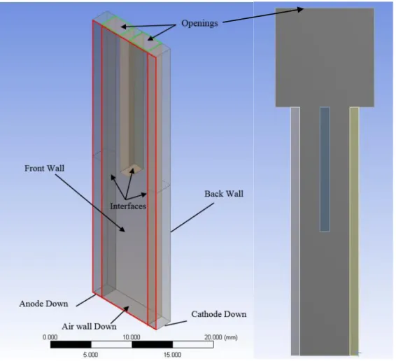
(37) During a circuit fault, the CB is turned off or is tripped, this interrupts the flow of current by separating its contacts. The current through the conductors of the CB generates a magnetic field in the arc chamber. The electromagnetic and thermal forces of the arc are supplemented to force the arc away from the contact region along arc runners and directly into the arc chutes. This assembly is made up of several “U” shaped steel plates that surround the contacts. As the arc develops, it is drawn into the arc chute where it is divided into smaller arcs, which are extinguished faster. Minimizing the arc is important for two reasons. First, arcing can damage the contacts. Second, the arc ionizes gases inside the molded case [15]. In turn, the current is reduced. Therefore, the arc cannot be maintained. The resistance of the arc and the arc voltage can be varied by increasing the length of the arc, cooling the arc and splitting the arc into a number of series arcs [16]. For more information about the arc physics, consult annex A.. 2.2.. Low voltage circuit breakers. A circuit breaker is a device designed not only to protect the load and cables but also for safety and security of the human life. All circuit breakers protect the circuit conductors mainly by detecting and interrupting the overcurrent [19]–[23]. The opening of the circuit breaker is a reaction to situations of transient current, such as short circuits or faults in the electrical system. The circuit breakers are classified according to the available interruption capacity and the nominal direct current (Low-voltage circuit breakers, Molded Case Circuit Breakers, (MCCB), Low Voltage Power Circuit Breakers (LVPCB), Isolated Circuit Breakers (ICCB), Mini Circuit Breakers (MCB) to mention a few) [24]. The interrupting capacity of a circuit breaker is the maximum short-circuit current that the circuit breaker can safely interrupt at a defined voltage. This short-circuit current described by current magnitude and its value is in symmetrical amperes rms. The amount of current that a circuit breaker can transmit until it reaches the overload conditions and opens the circuit is defined as the DC classification [25], [26],[27].. Interruption in LVCB At low voltage, the LVCBs are the most important devices for the extinction of electric arc. Most of them are very similar in layout design and structure, even though some differences exist. This way, the general layout of a conventional LVCB can be seen in Figure 2-3, including the following components:. 7.

(38) Figure 2-3 Double break rotary contact, Patent number: 8,159,319 B2..   . Upper connection: To connect the circuit breaker with the electrical circuit. Fixed and movable contacts: where the electric arc is formed when these contacts separate physically. Arc chamber and splitter plates stack: it is constituted by several plates, arranged in parallel between them. The aim is to split the arc into smaller arcs, in order to lengthen and extinguish it. In some references, the arc chamber is also known as arc chute.. Talking about conventional CB, generally use air for current interruption, with little differences in details and components, the general construction is showed in Figure 2-3, includes: the main contacts designed to carry the current under normal operating conditions, the arcing contacts (also called rails) the arc chamber, enclosure and the trip unit. In many cases, the geometry of the current carrying parts produces a magnetic force that moves the arc into the chamber. This way, some designs use coils for increasing the magnetic force, while others help the arc by blowing air [9]. The typical sequence in a LV conventional air circuit breaker is the following:      . The main contacts open while the arc contacts remain closed. The arcing contacts open and the arc starts to move along their length. The magnetic force produced by the arc current or by blowing coils moves the arc to the arc chamber. The arc is divided into several small arcs in series, by the plates of the arc chamber. he arc chamber allows cooling the arc, lengthening and narrowing its section until the current is interrupted. The arc chamber enables the ionization products to be dissipated or absorbed, restoring the dielectric strength in the air space between the contacts.. The conventional LVCBs described establish the arc in the interrupting medium, air in most LV switches, and maintain it until the next natural zero current for AC cases or until the voltage drop of the arc rises above circuit’s voltage for DC cases. Then, the arc is extinguished [9]. 8.

(39) 2.3.. The Limiter Circuit Breaker. As was mentioned below, to achieve a successful interruption, a CB must generate an arc voltage which in turn causes the arc to collapse. This kind of CB is known as Limiting Circuit-Breaker. A current limitation is achieved by making use of the arc voltage under fault conditions. This arc must be well managed, that is to say:  . The arc voltage must be sufficient value to facilitate high limitation and rapid extinction, Dielectric regeneration properties when the arc current reaches zero.. Further, the limiting CB must exhibit several properties under high short-circuit currents:    . A minimum current to ensure contact repulsion A transitive energy value, A short arc voltage duration, A maximum value of arc voltage, which is independent of the fault current.. The model also must take into account the external parameters of electric network being considered: voltage, frequency, short-circuit level, number of phases, etc. [28].. 2.3.1 Arc breaking The arc corresponds to a 4th physical condition: plasma. As soon as two contacts separate, one of them (cathode) transmits electrons and the other one (anode) receives them, and since electronic emission is by its very nature energy generating, the cathode will be hot (Figure 2-4). Resulting in arc stagnation which can give rise to metallic vapors. These vapors and the ambient gas will then be ionized, hence [28]:   . more free electrons; creation of positive ions which drop back on the cathode, thus maintaining its high temperature; creation of negative ions which bombard the anode causing temperature to rise.. Figure 2-4 the electric arc, composition of the arc column. [28]. 9.

(40) This natural phenomenon, once controlled, proved to be an irreplaceable intermediary for current breaking. Breaking control must relate to at least two specific arc-related aspects:  . Arc voltage helps reduce current strength and, Arc extinguishing conditions when the current moves to zero are met if dielectric regeneration is quickly achieved.. This regeneration must take place despite the presence of mains voltage and of the overvoltage phenomenon due to the circuit stray capacity (transient recovery voltage or TRV). The Figure 2-5 shows the TRV on breaking of DC and AC current. Consult annex A for more details about the arc physics. b. a. Ur  recovery voltage Ud  regeneration characteristics i  current at an instant t u  voltage at an instant t. Figure 2-5 Arc in extinguishing condition. a- in DC. voltage b- in AC. voltage with Ur of same sign as Ua at the time of zero current [28].. 2.3.2 Kind of breaking in established currents In both cases considered below (AC or DC), the current is in steady state before breaking. In a DC voltage As soon as the contacts open, an arc voltage appears and the current will start to decrease. The equation governing the circuit becomes: 𝑑𝑖. 𝑈𝑟 (𝑡) − 𝑅𝑖 − 𝐿 𝑑𝑡 − 𝑈𝑎 (𝑡) = 0. Ec. 2-1. Figure 2-6 equivalent circuit in a short circuit fault.. 10.

(41) It appears that current i cannot be forced to 0 unless arc voltage Ua becomes and remains greater than mains voltage E. Since the arc voltage is greater than mains voltage when the current is canceled, the resulting dielectric regeneration is problem free. Figure 2-6 shows an equivalent short-circuit fault. In an AC voltage In this case, the steady state current passes regularly via the zero value. The first condition to be reached is thus the quick dielectric regeneration of the arc when the current passes to zero, despite the presence of the mains voltage. Successful breaking is in practice a competition of speed between dielectric regeneration and evolution of mains voltage.. 2.3.3 Arc breaking with limitation “With limitation” means that measures are taken to prevent the short-circuit current having the time to reach its maximum value, (about 63% of maximum fault current). This current limitation will be obtained if arc voltage Ua quickly becomes greater than mains voltage and remains so until the current is canceled. In point of fact, the generalized Ohm´s law, (n is the number of splitters in the arc chamber and Ua is around 25-30 V [18]: 𝑑𝑖. 𝑈𝑟 − 𝑅𝑖 − 𝐿 𝑑𝑡 − 𝑛 ∙ 𝑈𝑎 (𝑡) = 0. Ec. 2-2. The Ec. 2-2 shows that di/dt will change sign as soon as Ua (t)>Ur (t) both in DC and AC voltage. Limitation devices are based on current effects beyond a certain threshold, the shortcircuit current creates thermal effects (fuse) or electromagnetic effects (circuit breakers) and generates an arc voltage [29].. 2.4.. Consequences of Arcing. The presence of an electric arc has both positive and negative consequences. The positive aspect is that the arc allows for a smooth decrease to zero current. If the circuit current were to suddenly drop to zero at the moment of contact separation, the energy stored in the inductance, L, would cause an over-voltage given by [18]: 𝑑𝐼. 𝑉 = −𝐿 𝑑𝑡. Ec. 2-3. The presence of an electric arc usually limits the over-voltage to a maximum of two or three times the circuit voltage. Without this feature, switch designers would have to design to protect the circuit against large over-voltages. However, other consequences of arcing could be devastating for the switching device and affect the design and choice of materials.. 2.4.1 Contact Erosion Since erosion of the contact material is one of the most important consequences of arcing and the design is directly relating to the lifetime of the device. It occurs because both the anode and cathode heats up to above the boiling temperature of the contact material. The 11.

(42) temperature of the arc is so high that erosion occurs even if the arc is moving across the contact surfaces. The amount of erosion depends on many parameters, for example:        . 2.5.. Circuit current Arcing time Open gap distance Contact material Size and shape of the contact Contact opening velocity Arc motion on the contacts Design of the arc chamber. Components of CB. Many of the principals used by circuit breaker engineers to analyze and design DC circuit breakers to interrupt DC currents are carried over from AC devices. The physics of open gap, arc runners, slot motors, reverse loops, and arc chutes also apply in DC systems. One might say that the use of these design strategies is even more demanding in DC circuit breakers due to the added burden of quenching the arc without the aid of a current crossing zero. The basic of circuit breaker design and construction, are created from the following five major components, Frame, Contacts, Arc Chute Assembly, Operating Mechanism and Trip Unit [1].. 2.5.1 Frame The frame provides an insulated housing to mount the circuit breaker components (Figure 2-7). The construction material is usually a thermal set plastic, such as glass-polymer. The construction material can be a factor in determining the interruption rating of the circuit breaker. Typical frame ratings include, maximum voltage, maximum ampere rating, and interrupting rating [30].. Figure 2-7 Frame of a Circuit Breaker [31].. 12.

(43) 2.5.2 Contacts The current flowing in a circuit controlled by a circuit breaker flows through the circuit breaker’s contacts. When a circuit breaker is turned off or is tripped by a fault current, the circuit breaker interrupts the flow of current by separating its contacts. Contacts are of two types depending on the interrupting rating: Straight-Through Contacts and Blow-Apart Contacts [30].. a) b) Figure 2-8 Straight through contacts and bow apart contacts [30].. Straight-Through Contacts Some circuit breakers use a straight-through contact arrangement, so called because the current flowing in one contact arm continues in a straight line through the other contact arm (Figure 2-8 a). Blow-Apart Contacts With this design, the two contact arms are positioned parallel to each other. As current flows through the contact arms, magnetic fields develop around each arm. Because the current flow in one arm is opposite in direction to the current flow in the other, the two magnetic fields oppose each other. Under normal conditions, the magnetic fields are not strong enough to force the contacts apart. When a fault develops, current increases rapidly causing the strength of the magnetic fields surrounding the contacts to increase as well (Figure 2-8 b).. 2.5.3 Arc Chute Assembly The arc is extinguished in this assembly. When a circuit breaker is turned off or is tripped by a fault current, the circuit breaker interrupts the flow of current by separating its contacts. This assembly is made up of several “U” shaped steel plates that surround the contacts (Figure 2-9). As the arc develops, it is drawn into the arc chute where it is divided into smaller arcs, which are extinguished faster [30].. 13.

(44) Figure 2-9 Arc chute assembly [30].. Minimizing the arc is important for two reasons. 1) Arcing can damage the contacts, 2) the arc ionizes gases inside the molded case. If the arc isn’t extinguished quickly the pressure from the ionized gases can cause the molded case to rupture.. 2.5.4 Operating Mechanism The operating handle is connected to the moveable contact arm through an operating mechanism. In the following illustration, the operating handle is moved from the “OFF” to the “ON” position Figure 2-10. In this process, a spring begins to apply tension to the mechanism. When the handle is directly over the center, the tension in the spring is strong enough to snap the contacts closed. This means that the speed of the contact closing is independent of how fast the handle is operated [30].. a). b). Figure 2-10 Operating mechanism, a) ON position, b) OFF position [30].. 2.5.5 Trip Unit In addition to providing a means to open and close its contacts manually, a circuit breaker must automatically open its contacts when an overcurrent is sensed. The trip unit (Figure 2-11), is the part of the circuit breaker that determines when the contacts will open automatically.. 14.

(45) Figure 2-11 Thermal-Magnetic trip unit [30].. In a thermal-magnetic circuit breaker, the trip unit includes elements designed to sense the heat resulting from an overload condition and the high current resulting from a short circuit. In addition, some thermal-magnetic circuit breakers incorporate a “Push-to-Trip” button [30].. 2.6.. Arc manipulation. Perhaps the most difficult aspect of designing a circuit interrupter is manipulating the arc such that it moves into the arc chute where it can be extinguished quickly and reliably. This can be accomplished by employing a variety of technologies, some common to AC and DC and some unique to DC [1].. 2.6.1. Open Gap The simplest method of DC circuit interruption is to use a large open gap. The open gap of a circuit breaker is defined as the distance between the movable and stationary contacts when they are fully parted. Another means of increasing open gap in a DC breaker is to wire multiple poles in series [1].. 2.6.2. Arc Runner Shortly after the introduction of the arc chute system, it was found that other techniques were required to guide the arc into the arc chute. One such guide is the arc runner (Figure 2-12). The arc runner is closely coupled to the main contacts. It attracts the arc drawing on the arc runner. Once the arc has reached the runner, it will remain on the arc runner provided that no lower resistance path occurs. Electromagnetic forces move the arc along the runner towards the arc chute [1].. 15.

(46) Splitter plates Arc chute. Arc Runners. Arcing contact. Arc. Main contacts. Figure 2-12 Assembling of arc runners [32].. 2.6.3. Blowout Coils This is a secondary copper coil in series with arcing contacts (Figure 2-13). The electromagnetic field helps move arc into arc chute. Contactors often incorporate magnetic blowout coils, for example, that push the arc away from the contacts as a means of more quickly cooling the arc [33].. Figure 2-13 Blowout coils assembling [34].. 2.6.4. Puffer As illustrated in the Figure 2-14 the breaker has a cylinder and piston arrangement. Here the piston is fixed but the cylinder is movable. The cylinder is tied to the moving contact so that for opening the breaker the cylinder along with the moving contact moves away from the fixed contact. But due to the presence of fixed piston the SF6 gas inside the cylinder is 16.

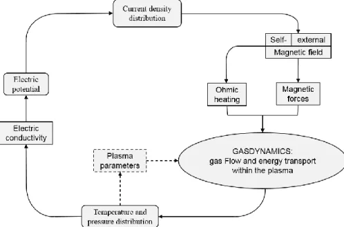
(47) compressed. The compressed SF6 gas flows through the nozzle and over the electric arc in the axial direction. Due to heat convection and radiation, the arc radius reduces gradually and the arc is finally extinguished at current zero [33].. Figure 2-14 Puffer type SF6 CB, a) ON position, b) OFF position [35].. 2.7.. Theory of Multi-physical Fields in a Fault Arc. The temperature of an arc fault could be over 20000 K. This may destroy electrical equipment and threaten human life [36]. Also, an arc fault can reach high levels of temperature, strong magnetic fields, added to mechanical stress and overpressure. In the present thesis, the multi-physical fields from the arc should be simulated to predict the complete phenomena in a simplified model of CB. To make this possible, the MagnetoHydrodynamics (MHD) Theory will be used to simulate the interaction of the plasma and the magnetic field density. The MHD refers to the interaction between an applied electromagnetic field and a flowing, electrically-conductive fluid. The MHD model allows analyzing the behavior of electrically conducting fluid flow under the influence of constant (DC) or oscillating (AC) electromagnetic fields [37]. With this approach, and with the current development of software tools, the physical processes that take place during the electric arc phenomenon is reproduced in detail. Even the methodology would can help us in the design and improvement of circuit breakers, being possible to study not only the parameters of the circuit, but also aspects directly related to the design, such as geometry, and main elements (as splitter plates or contacts), which are parameters studied by [24]. However, the major limitation of these models are:  . the limited accuracy in the resolution of the differential equations of the models, restriction in the computation time, 17.

(48)   . . need of a deep knowledge about the precise arc physical processes, knowledge of the physical properties of the extinguishing medium in a wide range of temperatures, also, test results from measurements of physical properties from the arc are needed to evaluate different parameters used, such as thermal conductivity, viscosity, electrical conductivity, specific heat or mass density, Geometry, mesh quality, resolution methods, convergence of results and experience of the engineer, also take an important role during the simulation process.. These aspects make the application of these type of models more difficult and determine the accuracy of the results provided by the model, [9]. With the MHD approach not only the equations of conservation of mass, momentum, and energy are considered in macroscopic elements, but also gas properties and empirical formulation to represent energy exchange mechanisms during the simulation. However, they all require applying simplifications in relation to the geometry and physical properties of the arc plasma. The thesis presented by [9] follows the next assumptions to adopt in current physical models:  .   .   . . Arc plasma is electrically neutral and is represented as a mixture of gases at high temperature. There is a thermodynamic equation of state for each component of the plasma (electrons, ions, atoms and molecular species), but it is usually neglected in the macroscopic scale analysis. Physical properties of plasma (thermal conductivity, viscosity, density, specific heat, electrical conductivity) depend on its temperature and pressure conditions. The behavior of the gaseous mass is described by applying the Navier Stokes’ (conservation of mass, momentum, and energy) and Maxwell's equations. Since plasma is electrically conductive, the corresponding term for the interaction with the magnetic field must be considered in the momentum equation. This magnetic field, depending on the degree of accuracy of the model, can be defined as external or self-induced by the current flowing through the arc. The second option is closer to reality. The magnetic field is calculated by applying Biot-Savart or by calculating the magnetic vector potential once the current distribution is known. The energy conservation equation is modified by considering additional terms that represent the generation of heat by Joule effect and the heat dissipation by radiation. In many cases, local thermal equilibrium (LTE) is assumed for the plasma, so that it is possible to set a temperature value which determines the degree of dissociation and ionization. The initialization of the arc is not achieved by the dynamic movement of the electrodes separation, as in reality, due to the complexity. The arc/electrode interaction is not considered in a microscopic way. 18.

(49) The last one considerations, make it possible to obtain the MHD equations for fluids under the influence of electromagnetic fields.. 2.8.. Fluid Models Magnetohydrodynamic description. The huge number of particles makes it impossible to solve Newton’s equation for each of these particles. The magneto-hydrodynamic definition provides information about the behavior of the electric arc, by fluid dynamics and thermodynamic laws, at a macroscopic scale [9]. To understand the background of the MHD it is necessary to see the electric arc as a collection of particles.    . Electrons, Ions, Atoms and, Molecular species.. But the solution of all of them leads to a quite large mathematical problem. Accordingly, it is necessary to group all these particles into two categories, (or as two fluids):  . heavy particles (ions and neutrals) and light particles (electrons). Each one is characterized by its own temperature: Te (temperature of the electrons) and Ta (temperature of the heavy particles). In the vicinity of the electrodes, (named cathode and anode regions), in a very thin surface layer, temperature falls from the value of the plasma column (typically around 25000K) to the value of the electrode (typically around 3000K). With that temperature of the electrode, the electrical conductivity value is close to zero, so that no current should flow, but the electrode is the main supplier of current to the plasma. This contradiction is solved taking into account that in unbalanced plasmas or without thermal equilibrium, the two previously mentioned temperatures appear. While the temperature of the heavy particles falls, the temperature of electrons is maintained at a high value, so that the plasma keeps being conductor in the situations described. However, if extinction and reignition are not considered in the analysis, and the arc roots are macroscopically solved, it is possible to simulate the evolution of the arc at a macroscopic scale, by the approach called magneto-hydrodynamics. Which considers the plasma as a single fluid [9]. With the last considerations, the MHD method is used to calculate a plasma in Local Thermic equilibrium (LTE), in [9] are mentioned some considerations to assume this.   . Thermal equilibrium: the electrons temperature Te, is equal to (or very similar) the heavy particles temperature Ta. Ionization equilibrium: the electron density, ne, is equal or very similar to the density of electrons na that would exist in the plasma, with a unique temperature. Quasi-neutrality: the plasma is electrically neutral, both globally and locally. 19.

(50) Nevertheless, in the case of LV arcs the three above assumptions are not fulfilled in the arc roots, neither in the zero current when the arc is extinguished. For those reasons arc roots are not going to be analyzed deeply, just in a macroscopic way. Thus, adopting the LTE hypothesis and, therefore, adopting a single temperature field, “T”, and a single average velocity field for the fluid "u", for the whole plasma, that plasma can be reduced to a single fluid, simplifying the state equations of each particle [9]. Given the foregoing considerations, transport equations for the conservation of mass, momentum and energy of the plasma as a single fluid are defined, which are known as the modified Navier-Stokes equations, (Ec. 2-3 – Ec. 2-5).. 2.9.. Simulation tool.. The previous explanation gives the background about the behavior of an electric arc, now it is time to choose the computational tool to solve the problem. In this thesis were chosen the next software with some of their characteristics.. 2.9.1 Ansys-Fluent. ANSYS Fluent is a computer program for modeling fluid flow, heat transfer, and chemical reactions with complex geometries. Fluent uses the Volume of Fluid method (VOF), Mixture model or Eulerian model to solve the transport equations. The fluid flow conserves mass, momentum and energy are solved in ANSYS Fluent for a fluid flow. The mass conservation equation can be written as follows: [36] 𝜕𝜌 𝜕𝑡. + 𝛻 ∙ (𝜌𝑽) = 0. Change rate of density in the control volume. Ec. 2-4 [9]. Difference between the incoming and outgoing mass flow in the control volume. The momentum conservation is described by: 𝜌. 𝜕(𝑽) 𝜕𝑡. 4. + 𝜌(𝑽 ∙ 𝛻)𝑽 = −𝛻𝑝 + 3 𝛻𝜇(𝛻 ∙ 𝑽) − 𝛻𝘹𝜇(𝛻𝘹𝑽) + 𝑭 + 𝜌𝒈. Change rate of momentum in the volume control Momentum difference in the incoming and outgoing flow in the control volumen. Pressure gradient. Lorentz force. Interaction term with the magnetic field. Surface forces on the control volume. 20. Accelerating gravity force. Ec. 2-5 [9].

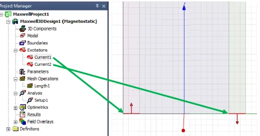
(51) The equation for energy conservation is given by 𝜕. 𝜕𝑝. 𝐾. 𝜌 𝜕𝑡 (𝐻) + 𝜌(𝑽 ∙ 𝛻)𝐻 − 𝜕𝑡 − (𝑽 ∙ 𝛻𝑝) = 𝛻 ∙ 𝐶 𝛻𝐻 − 𝛻 ∙ 𝒒𝑹 + 𝛷 + 𝑆ℎ 𝑝. Variation rate of enthalpy in the control volume. Work produced by the pressure change and pressure gradient. Ohmic heating input in the CV. Radiative heat loss. Enthalpy difference in the incoming and outgoing flow in the control volume. Conductive heat loss. Ec. 2-6 [9]. Viscous dissipation term. Being Φ the viscous dissipation factor (usually neglected), expressed as: 𝛷 = ∑ [𝜇 (. 𝜕𝑣𝑖. 𝜕𝑥𝑗. +. 𝜕𝑣𝑗 𝜕𝑥𝑖. 2. )− 𝜇 3. 𝜕𝑣𝑘 𝜕𝑣 𝛿 ] 𝑖 𝜕𝑥𝑘 𝑖𝑗 𝜕𝑥𝑗. Ec. 2-7 [9]. Where: ρ: 𝐕: t: p: μ: g: H: K: Cp : T:. gas density gas velocity time pressure viscosity gravity acceleration gas enthalpy thermal conductivity specific heat at constant pressure temperature. The source term in the fluid momentum equation is the Lorentz force given by: 𝑭 = 𝑱𝘹𝑩. Ec. 2-8. where the magnetic field is 𝑩 = 𝛻𝛸𝑨 The source term, Sh, includes the Joule heating rate given by: 𝑆ℎ = 𝑄 =. 𝑱𝟐 𝜎. = 𝑱 ∙ 𝑬 Ec. 2-9. 2.9.2 ANSYS-Maxwell. ANSYS Maxwell is the industry-leading electromagnetic field simulation software for the design and analysis of electric motors, actuators, sensors, transformers and other electromagnetic and electromechani-cal devices. Maxwell uses the accurate finite element method to solve static, frequency-domain and time-varying electromagnetic and electric fields [38]. In this thesis, Maxwell must calculate the electromagnetic fields from the multi-physical fields in a fault arc. This can be reached by the coupling of Maxwell and ANSYS-Fluent, so that, Fluent makes a mapping of the electric conductivity of the fluid and export this to 21.

(52) Maxwell to calculate the magnetic flux density B. Electromagnetic fields are described by Maxwell’s equations: Magnetic field Gauss´ law. 𝜵∙𝑩=𝟎. Faraday´s law. 𝛻𝘹𝑬 = − 𝜕t. Gauss´ law. 𝛻∙𝑫 = q. Ec. 2-10. 𝜕𝑩. Ampere´s generalized law. 𝛻𝘹𝑯 = 𝑱 +. Ec. 2-11 Ec. 2-12. 𝜕𝑫 𝜕t. Ec. 2-13. Where: 𝑱: 𝑩: E: D: H: q:. current density magnetic flux density electric field electric field density magnetic induction field electric charge density. B (Tesla) and E (V/m) are the magnetic and electric fields, respectively, and H and D are the induction fields for the magnetic and electric fields, respectively. q (C/m3) is the electric charge density, and J (A/m2) is the electric current density vector. With the last equations it is proceeding to reduce some terms, and adding other like the Lorentz forces and the Joule heating, and to facilitate understanding the energy conservation equation is changed to temperature terms, remaining as shown below. Mass conservation equation. 𝜕𝜌 𝜕𝑡. + 𝛻 ∙ (𝜌𝑽) = 0. Ec. 2-14. Momentum conservation equation. 𝜌. 𝜕(𝑽) 𝜕𝑡. 4. + 𝜌(𝑽 ∙ 𝛻)𝑽 = −𝛻𝑝 + 3 𝛻𝜇(𝛻 ∙ 𝑽) − 𝛻𝘹𝜇(𝛻𝘹𝑽) + 𝑱𝘹𝑩. Ec. 2-15. Energy conservation equation. 𝜕𝑇. 𝜕𝑝. 𝜌𝐶𝑝 ( 𝜕𝑡 ) + 𝜌𝐶𝑝 (𝑽 ∙ 𝛻)𝑇 = 𝛻 ∙ (𝑘𝛻𝑇) + 𝜕𝑡 + (𝑽 ∙ 𝛻𝑝) − 𝛻 ∙ 𝒒𝑹 + 𝑱 ∙ 𝑬. Ec. 2-16. 2.9.3 Altair-Flux Flux is the leading software for electromagnetic. This software uses the Finite Element Method techniques to solve the electromagnetic equations in the model. Flux has a module where it can simulate transient magnetic and steady-state AC phenomena, in its user’s guide documents [39]. 22.