CO2 with Mechanical Subcooling vs CO2 Cascade Cycles for Medium Temperature Commercial Refrigeration Applications Thermodynamic Analysis

Texto completo

(1)applied sciences Article. CO2 with Mechanical Subcooling vs. CO2 Cascade Cycles for Medium Temperature Commercial Refrigeration Applications Thermodynamic Analysis Laura Nebot-Andrés *, Rodrigo Llopis. ID. , Daniel Sánchez, Jesús Catalán-Gil and Ramón Cabello. Department of Mechanical Engineering and Construction, Jaume I University, Campus de Riu Sec s/n, Castellón de la Plana, E-12071, Spain; [email protected] (R.L.); [email protected] (D.S.); [email protected] (J.C.-G.); [email protected] (R.C.) * Correspondence: [email protected]; Tel.: +34-964-72-8133; Fax: +34-964-728106 Received: 24 July 2017; Accepted: 11 September 2017; Published: 16 September 2017. Abstract: A recent trend to spread the use of CO2 refrigeration cycles in warm regions of the world is to combine a CO2 cycle with another one using a high performance refrigerant. Two alternatives are being considered: cascade and mechanical subcooling systems. Both respond to a similar configuration of the refrigeration cycle, they being based on the use of two compressors and same number of heat exchangers. However, the compressor, heat exchanger sizes and energy performance differ a lot between them. This work, using experimental relations for CO2 and R1234yf semi-hermetic compressors analyzes in depth both alternatives under the warm climate of Spain. In general, it was concluded that the CO2 refrigeration solution with mechanical subcooling would cover all the conditions with high overall energy efficiency, thus it being recommended for further extension of the CO2 refrigeration applications. Keywords: CO2 ; transcritical; cascade; mechanical subcooling; energy efficiency. 1. Introduction Carbon dioxide was spread out all over the world as refrigerant because it combines excellent environmental (GWP = 1) and safety properties (A1), despite its differences in regards to traditional refrigerants, such as high working pressures, low critical temperature and high densities. After the approval of the F-Gas Regulation [1] in Europe in 2014, the implication in the industry with this refrigerant was taken a step forward, especially in commercial refrigeration, whose systems are extreme energy consumers and commonly characterized by large leakage rates of refrigerant. Regarding the environmental impact, the use of CO2 practically eliminates the direct effect of the refrigeration system, thanks to its low GWP. However, the indirect impact associated with the energy consumption of the plant is an issue still under analysis and contrast among the scientific community and the industry sector. In cold regions of the planet, with low average annual temperatures below 14–15 ◦ C, the standard CO2 cycles perform with energy efficiency levels higher than the conventional HFC-based plants [2]. However, when the environment temperature rises, the standard CO2 systems [3] are not able to reach the performance of the formers, and thus, advanced and more complex systems must be considered to be able to mitigate indirect impact of the system. The search for improvements in CO2 standard refrigeration cycles follow two main directions: new components and the combination of CO2 cycles with other systems. Regarding new components, the CO2 expander concept is still under maturation, few experimental works were found in the literature, such as the experimental tests with a rotary vane expander of Jia et al. [4] and with a two-rolling piston expander of Hu et al. [5]. However, great progress was achieved in the last decade regarding the ejector technology; it was already implemented in many plants all over the world, Appl. Sci. 2017, 7, 955; doi:10.3390/app7090955. www.mdpi.com/journal/applsci.

(2) Appl. Sci. 2017, 7, 955. 2 of 22. where the energy improvements were experimentally demonstrated [6]. Now, research on ejector technology is focused on achieving adaptable ejectors to all the operation range of the plants, such as the multi-ejector concept of Hafner et al. [7] or the adjustable ejector concept of Lawrence and Elbel [8], among others. On the other side, scientists and industry are working on the thermal integration of CO2 refrigeration cycles with other energy systems to obtain higher overall energy efficiency to make CO2 more competitive. The attempts correspond to the integration of the CO2 refrigeration plants with water heating systems and air conditioning systems [9], desiccant wheels [10], absorption plants [11], etc.; where in all the cases important overall increases of the energy efficiency were achieved. Another type of CO2 combined refrigeration system, widely implemented in the last decade in the commercial sector, is the cascade system using CO2 as low temperature refrigerant [12]. This combination corresponds to the thermal coupling of two single stage cycles working with different refrigerants, where the high temperature cycle keeps the CO2 low temperature cycle always in subcritical conditions, thus avoiding the high operating pressures of CO2 and the need for regulation of the high pressure in transcritical conditions [13]. As analyzed by Llopis et al. [14], this cycle overcomes the energy efficiency levels of standard CO2 refrigeration cycles and it reaches comparable coefficient of performance (COP) values than the current systems in commercial refrigeration at low evaporation levels and high environment temperatures. In addition, from the point of view of environmental impact, this system presents low values of TEWI among the solutions adapted to the new F-Gas Regulation. Similar to the cascade solution, since the operating cycle is equivalent, another CO2 combined cycle is attracting attention in the last years, the thermal joining of a CO2 cycle with a dedicated mechanical subcooling system. This option was studied from a theoretical point of view by Hafner et al. [15], Gullo el. at. [16] and Llopis et al. [17], and from an experimental point of view by Nebot-Andrés et al. [18] and Eikevik et al. [19]. This cycle is characterized by a main refrigeration cycle working with CO2 that can be operated in subcritical or transcritical modes which is helped by another vapor compression system, the dedicated mechanical subcooling cycle, providing CO2 a large subcooling at the exit of the gas-cooler/condenser. The benefits of this combination are a large increment of the cooling capacity, reductions of the optimum CO2 high working pressure and an important increment of the overall energy efficiency. Nebot-Andrés et al. [18], for an evaporation level of 0 ◦ C, increments on cooling capacity of 34.9% were measured and, referring to COP, increments of 22.8% at 30.2 ◦ C of heat rejection temperature. At 40 ◦ C of heat rejection temperature, the increments are 40.7% of cooling capacity and 17.3% of COP. These increments are calculated considering a single-stage CO2 transcritical plant without internal heat exchanger as base line. These last approaches, i.e., the cascaded CO2 and the subcooled CO2 solutions, are being considered to spread the use of CO2 in centralized refrigeration systems at a medium temperature level in medium to warm regions of the planet such as Spain or Italy. As mentioned, both refrigeration schemes have similar configuration of the refrigeration cycle: one rack of compressors for the CO2 and another for the high temperature/subcooling cycle and same number of heat exchangers. However, they have differences in the operation of the components that compose the cycle. One of the main differences, which is discussed in Section 2, is that the high-pressure CO2 heat exchangers can operate as single-phase/two-phase or two-phase/two-phase (cascade) heat exchangers, being the heat transfer rate different in each operating mode. This work aims to analyze which cycle configuration (cascade or mechanical subcooling) is recommended for different operating conditions. The analysis is based on simplified models close to reality, since they use real performances of the compressors. The comparison provides clear conclusions about the application range, advantages and disadvantages of each cycle. In the paper, first, the optimum operating conditions of each cycle are established; then for the optimum conditions, the reached COP values and the ratio of electrical consumption of the compressors are presented. Next, energy efficiency results of both solutions are merged to determine at which operating conditions each solution is the best performing system. Finally, both systems are evaluated under the different climate conditions of Spain to obtain clear conclusions about their possible implementation..

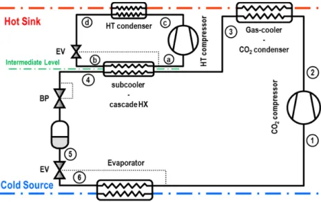
(3) Appl. Sci. 2017, 7, 955. 3 of 22. 2. Refrigeration Cycles, Models and Assumptions The Sci. cascade refrigeration cycle and the mechanical subcooling (MS) cycle can be represented by Appl. 2017, 7, 955 3 of 22 the refrigeration scheme detailed in Figure 1. Essentially, both systems include these main components Refrigeration Cycles, Models and Assumptions with 2. the following operating characteristics:. • • • • • •. The cascade refrigeration cycle and the mechanical subcooling (MS) cycle can be represented by. A cycle, working CO2 as which absorbs the cold themain refrigeration schemewith detailed in refrigerant, Figure 1. Essentially, both energy systemsfrom include thesesource. main A CO2 compressor, subcritical-rated the cascade configuration and transcritical-rated for the components with the following operatingfor characteristics: MS configuration.  A main cycle, working with CO2 as refrigerant, which absorbs energy from the cold source. A CO gas-cooler, which performs heat rejection to the hot sink.  A2CO 2 compressor, subcritical‐rated for the cascade configuration and transcritical‐rated for the A second CO heat exchanger acting as CO2 condenser for the cascade system and as CO2 MS configuration. 2 subcooler the MS which configuration.  A CO2 for gas‐cooler, performs heat rejection to the hot sink.  expansion A second CO 2 heat composed exchanger acting CO2 + condenser forvalve’ the cascade andconfiguration as CO2 An system: of the as ‘vessel expansion for thesystem cascade subcooler for the MS configuration. and of a ‘back-pressure + vessel + expansion valve’ for the MS cycle.  An expansion system: composed of the ‘vessel + expansion valve’ for the cascade configuration An auxiliary single-stage refrigeration cycle: working with another refrigerant (HCs, HFOs, NH3 , and of a ‘back‐pressure + vessel + expansion valve’ for the MS cycle. HFCs) as high temperature cycle in the cascade configuration and as dedicated mechanical  An auxiliary single‐stage refrigeration cycle: working with another refrigerant (HCs, HFOs, subcooling cycle asforhigh the temperature MS configuration. system, whose NH3, HFCs) cycle in The the auxiliary cascade configuration and refrigerant as dedicatedis not distributed to the cooling appliances, absorbs heat from the intermediate temperature mechanical subcooling cycle for the MS configuration. The auxiliary system, whose refrigerant level and is performs heat rejection to the same hot sink as theheat main cycle. In the cascade configuration, not distributed to the cooling appliances, absorbs from the intermediate temperature level andcycle performs heat CO rejection to the same hot sink as the main cycle. In the cascade the auxiliary performs condensation and in the MS it only subcools the CO 2 2 at the exit configuration, of the gas-cooler. the auxiliary cycle performs CO2 condensation and in the MS it only subcools the CO2 at the exit of the gas‐cooler.. The operation of the cycle of Figure 1 as cascade or as MS cycle will depend on the hot sink The operation of the cycle of Figure 1 as cascade or as MS cycle will depend on the hot sink temperature (TH )(Tand on the high-pressure fixed by the back-pressure valve (P), as),detailed as detailed in the temperature H) and on the high‐pressure fixed by the back‐pressure valve (Phighhigh in the following subsections. following subsections.. Figure 1. Schematic representation of cascade and CO2 with mechanical subcooling.. Figure 1. Schematic representation of cascade and CO2 with mechanical subcooling.. 2.1. CO2 Refrigeration Cycle with Mechanical Subcooling (MS Cycle). 2.1. CO2 Refrigeration Cycle with Mechanical Subcooling (MS Cycle). Essentially, the CO2 refrigeration cycle with mechanical subcooling corresponds to a main CO2 single‐stage that2 uses an auxiliary cycle, with small capacity, to provide subcooling to at the exit CO2 Essentially,cycle the CO refrigeration cycle with mechanical subcooling corresponds a main of the gas‐cooler/condenser [17]. This cycle operates in subcritical or transcritical conditions single-stage cycle that uses an auxiliary cycle, with small capacity, to provide subcooling at the exit of depending on the heat rejection temperature (TH) and on the high‐pressure established by the the gas-cooler/condenser [17]. This cycle operates in subcritical or transcritical conditions depending back‐pressure valve (Phigh). on the heat rejection temperature (TH ) and on the high-pressure established by the back-pressure The transition from subcritical to transcritical conditions was investigated by Ge et al. [20], Shao valveet(P ). Tsamos el at. [22] and Sanchez et al. [23] for standard CO2 refrigeration cycles, however, no al.high [21], The transition from subcritical towhen transcritical conditions was investigated bysystem. Ge etFor al. [20], reference for the transition was found the CO2 cycle uses a mechanical subcooling Shaothe et al. [21], Tsamos el cycle, at. [22] Sanchez et al. [23] for standard CO2was refrigeration however, analysis of the MS theand transition from transcritical to subcritical establishedcycles, in terms of.

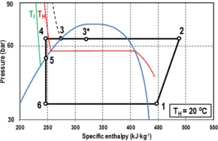
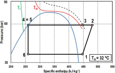
(4) Appl. Sci. 2017, 7, 955. 4 of 22. no reference for the transition was found when the CO2 cycle uses a mechanical subcooling system. For the analysis of the MS cycle, the transition from transcritical to subcritical was established in terms of the maximum COP value reached by each operating mode although this transition in real plants would beSci. difficult. The considerations are the following: Appl. Sci. 2017, 7, 7, 955 955 of 22 22 Appl. 2017, 44 of If saturation pressure of CO2 at TH is lower than the pressure fixed by the back-pressure (Phigh ) and the is maximum COP value reached by each each operating mode although this transition transition in real real plants will the maximum COP value reached by operating mode this in plants this last lower than the critical pressure of CO bar),although the optimum operation conditions 2 (73.773 would be difficult. The considerations are the following: be difficult. The are theThese following: be inwould subcritical-mode withconsiderations liquid subcooling. boundary conditions are detailed by Equation (1), If saturation saturation pressure pressure of of CO CO22 at at T THH is is lower lower than than the the pressure pressure fixed fixed by by the the back‐pressure back‐pressure (P (Phigh high)) If and the corresponding pressure-enthalpy diagram of CO 2 represented in Figure 2. In this type of and this last is lower than the critical pressure of CO 2 (73.773 bar), the optimum operation conditions and this last is lower than the critical pressure of CO2 (73.773 bar), the optimum operation conditions operation, the first CO2 heat exchanger acts as condenser (point 2 to 3) and the subcooler subcools will be be in in subcritical‐mode subcritical‐mode with with liquid liquid subcooling. subcooling. These These boundary boundary conditions conditions are are detailed detailed by by will liquidEquation CO2 (points 3 tothe 4).corresponding The case of partial condensation in the of CO exchanger (point 2. 2 to 2 heat (1), and pressure‐enthalpy diagram CO 2 represented in Figure In 3*) is Equation (1), and the corresponding pressure‐enthalpy diagram of CO2 represented in Figure 2. In possible, but of the best energy results obtained foracts complete condensation. this type type of operation, operation, the first first CO22are heat exchanger acts as condenser condenser (point 22 to to 3) 3) and and the the subcooler subcooler this the CO heat exchanger as (point subcools liquid liquid CO CO22 (points (points 33 to to 4). 4). The The case case of of partial partial condensation condensation in in the the CO CO22 heat heat exchanger exchanger (point (point subcools P T < P ≤ P ( ) sat,CO H crit,CO 2 to 3*) is possible, but the best energy results are obtained for complete condensation. high 2 2 2 to 3*) is possible, but the best energy results are obtained for complete condensation. (1) (1) P ,, T P P ,, P > P crit,CO2 (2) P Phigh, (2) ,. (1) (2). For pressures fixed byby thethe back-pressure higherthan than critical pressure, Equation high)) )higher higher than thethe critical pressure, Equation (2), (2), For pressures pressures fixed by the back‐pressure (P (Phigh high the critical pressure, Equation (2), For fixed back‐pressure (P the optimum operating conditions mode,as represented Figure 3. this For this the optimum optimum operating conditionsare arein in transcritical transcritical mode, mode, asasrepresented represented by by Figure 3. For For this the operating conditions are in transcritical by Figure 3. mode of operation, operation, the first CO 2 heat heatexchanger exchanger acts acts as gas‐cooler (point to23) 3) and the subcooler subcooler modemode of operation, thethe first CO actsas asgas‐cooler gas-cooler (point toand 3) and the subcooler 2 2heat of first CO exchanger (point 22 to the subcools gas or liquid liquid depending on the high‐pressure high‐pressure and THH temperature temperature (in red). The subcools gas or liquid depending on theon high-pressure and THand temperature (in red).(in Thered). intermediate subcools gas or depending the T The intermediate temperature (T I ) corresponds to the evaporating level of the high pressure cicle, in intermediate temperature (T corresponds to the of thecicle, highinpressure cicle, temperature (TI ) corresponds toI)the evaporating levelevaporating of the highlevel pressure green, and is in always green, and is always lower than T H . lowergreen, thanand TH .is always lower than TH.. Figure 2. Pressure‐enthalpy Pressure‐enthalpy diagramof ofmechanical mechanical subcooling subcooling (MS) cycle in subcritical subcritical conditions. Figure 2. Pressure-enthalpy diagram subcooling(MS) (MS) cycle in subcritical conditions. Figure 2. diagram of mechanical cycle in conditions.. Figure 3. Pressure-enthalpy ofMS MScycle cyclein transcritical conditions. Figure 3. Pressure‐enthalpy Pressure‐enthalpydiagram diagram of of MS cycle inin transcritical conditions. Figure 3. diagram transcritical conditions.. 2.2. Cascade Cascade Refrigeration Refrigeration Cycle Cycle 2.2..

(5) Appl. Sci. 2017, 7, 955. Appl. Sci. 2017, Refrigeration 7, 955 2.2. Cascade. 5 of 22. 5 of 22. Cycle. Cascade refrigeration combination of of twotwo main refrigeration cycles, one Cascade refrigeration cycle cyclecorresponds correspondstotothe the combination main refrigeration cycles, cycle working with CO in the low temperature level, which is condensed and maintained in subcritical, 2 CO2 in the low temperature level, which is condensed and maintained in one cycle working with by another cycle that uses a refrigerant good performance high evaporation subcritical, by another cycle that uses awith refrigerant with good at performance at hightemperatures. evaporation In this case, both cycles are necessary, since the operation of the low temperature cycle depends on temperatures. In this case, both cycles are necessary, since the operation of the low temperature cycle the operation of the high temperature cycle. In addition in this case, the high temperature cycle has depends on the operation of the high temperature cycle. In addition in this case, the high similar or higher capacity than the low temperature temperature cyclecooling has similar or higher cooling capacity thancycle. the low temperature cycle. Figure 4 represents the operation of the CO cycle in This is is the the mode mode of of Figure 4 represents the operation of the CO22 cycle in aa cascade cascade system. system. This operation if the condition established by Equation (3) or Equation (4) is satisfied. That is, when the operation if the condition established by Equation (3) or Equation (4) is satisfied. That is, when the pressure established established by by the the back‐pressure back-pressure (if (if present) present) or or by by the the thermal thermal equilibrium equilibrium of of condensation condensation pressure (P ) is lower than the CO saturation pressure at T , Equation (3). As established in Equation high) is lower than the CO2 2saturation pressure at TH,HEquation (3). As established in Equation (Phigh (4),(4), if ifHTis higher than thecritical criticaltemperature temperatureofofCO CO2,2 ,the thehigh‐pressure high-pressure (P (Phigh mustbe belower lower than than the the H is high T higher than the ) )must critical one one to to satisfy satisfy the the condition. condition. critical. P Phigh <PPsat,CO TH ) ifif TTH ≤ TTcrit,CO (T , , 2 , OR , OR 2 P Phigh <PPcrit,CO if TTH >Tcrit,CO T , , if 2 2. (3) (3) (4) (4). then the In rejection to to T TH and In the the subcritical subcritical mode, mode, the the gas‐cooler gas-cooler performs performs aa small small heat heat rejection H and then the high‐temperature cycle condenses CO 2 until saturated liquid. Subcooling is possible, but it offers high-temperature cycle condenses CO2 until saturated liquid. Subcooling is possible, but it offers worse exit in in saturation saturation conditions conditions because because the intermediate temperature worse results results than than the the exit the intermediate temperature will will need need to descend. to descend. This experimentally investigated by Dopazo et al. [24] using 3/CO2 and Sanz et al. This cycle cyclewas was experimentally investigated by Dopazo et al. [24]NH using NH3 /CO2 and [12] using HFC134a/CO 2. Sanz et al. [12] using HFC134a/CO . 2. Figure 4. Pressure-enthalpy diagram of the low temperature cycle (CO2 ) of the cascade. Figure 4. Pressure‐enthalpy diagram of the low temperature cycle (CO2) of the cascade.. 2.3. Calculation Calculation Models Models and and Assumptions Assumptions 2.3. We performed of of thethe MSMS andand the cascade cyclescycles using using simplified but realistic models, We performedthe theanalysis analysis the cascade simplified but realistic which assumptions are detailed then. models, which assumptions are detailed then. CO22 compressor is modeled using the overall efficiency as a linear CO compressor for forboth bothconfigurations configurations is modeled using the overall efficiency as arelation linear with the compression ratio, as detailed by Equation (5). We fitted this relation using experimental data relation with the compression ratio, as detailed by Equation (5). We fitted this relation using of a semi-hermetic single-stage CO compressor able to operate in subcritical or transcritical [23]. 2 experimental data of a semi‐hermetic single‐stage CO2 compressor able to operate in subcritical or. transcritical [23].. η. ηG,CO2 = 0.7359 − 0.0517tCO2 ,. 0.7359. 0.0517t. (5) (5). For either the MS and cascade configurations, an approach temperature in gas‐cooler of 5 K regards the environment temperature and 10 K of superheating degree in evaporator are chosen. For the MS configuration, when working in transcritical conditions, the high‐pressure is established by the back‐pressure. The tunable parameters are the high‐pressure and the subcooling degree in.

(6) Appl. Sci. 2017, 7, 955. 6 of 22. For either the MS and cascade configurations, an approach temperature in gas-cooler of 5 K regards the environment temperature and 10 K of superheating degree in evaporator are chosen. For the MS configuration, when working in transcritical conditions, the high-pressure is established by the back-pressure. The tunable parameters are the high-pressure and the subcooling degree in subcooler (SUB = T3 − T4 ). Both parameters are optimized to obtain the best performing conditions. When working in subcritical, high pressure is computed as saturation temperature of CO2 at the environment temperature plus a temperature difference in condenser of 5 K, to maintain the same reference level as in transcritical. The exit of the condenser is considered in saturation. Only the subcooling degree in the subcooler is free, it being optimized in the calculations. For the cascade configuration, the tunable variable is the temperature of the intermediate level, being the CO2 condensing temperature taken as reference and optimized in the calculations. In this case, the exit condition of CO2 of the cascade heat exchanger is considered in saturation. For both cycles, the lamination processes are assumed isenthalpic and pressure losses and heat transfer to the environment in the lines are neglected. Regarding the secondary refrigerant, R1234yf is selected for the MS cycle and for the high-temperature cycle. This HFO is one of the new generation of refrigerants introduced to the market with the aim of substitute the R134, being an alternative with low GWP but light inflammable (A2L), that can perform as drop-in replacement. Aprea et al. [25] find out that this drop-in allows increasing the cooling capacity, being a refrigerant suitable for new plants and plants that are already working. The overall efficiency of the compressor is also adjusted as a linear relation with the compression ratio, as detailed by Equation (6), in this case fitted from experimental data of a semi-hermetic compressor [26]. ηG,R1234yf = 0.9721 − 0.0533tR1234yf (6) The high-temperature cycle or dedicated mechanical subcooling cycle, is thermally linked to the CO2 cycle using two different approaches: when working as condenser in the cascade configuration, the evaporation temperature of R1234yf is considered to be 5 K below the CO2 condensing temperature [12], thus being optimized during the calculation. On the other hand, when this cycle operates as mechanical subcooler, its evaporation temperature is computed considering a thermal effectiveness of the subcooler of 60%, Equation (7), being this effectiveness the average value measured in [27]. This temperature is indirectly optimized by tuning of the optimum subcooling degree in the CO2 cycle. To,R1234yf,MS = T3 −. SUB T − T4 = T3 − 3 ε ε. (7). For this cycle, a degree of superheat in the evaporator of 5 K is chosen. The exit of the condenser is in saturation and the expansion process is isenthalpic. Also, pressure losses and heat transfer to the environment in pipes are neglected. The relation between the refrigerant mass flow rates of both cycles is obtained through the energy balance in the subcooler/cascade HX as established by Equation (8) according to nomenclature of Figure 1. . mR1234yf h − h4 = 3 (8) . ha − hb mCO2 Using relation (8), the main energy parameters can be expressed as a function of the refrigerant enthalpies and the overall efficiencies of the compressors. Equation (9) expresses the overall COP of the cycle combination as quotient between the cooling capacity of the CO2 cycle and the sum of power consumptions of both compressors. Equation (10) establishes the relation between the power.

(7) Appl. Sci. 2017, 7, 955. 7 of 22. consumption of the MS/cascade compressor regards the power consumption of the CO2 compressor, it being an indicative of the size of the auxiliary cycle. .. COP =. PC,CO2. QO h1 − h4 = h2,s − h1 h3 − h4 hc,s − ha + PC,R1234yf + × ηG,CO2 ha − hb ηG,R1234yf. PC,R1234yf ηG,CO2 (h − h4 ) × (hc,s − ha ) × = 3 PC,CO2 (ha − hb ) × (h2,s − h1 ) ηG,R1234yf. (9). (10). All the thermophysical properties of the refrigerants have been calculated using Refprop database [28]. 3. Results This section establishes the optimum operating conditions of the CO2 refrigeration cycle with mechanical subcooling (Section 3.1) and of the cascade cycle using CO2 as low temperature fluid (Section 3.2) using the model detailed in Section 2. The evaluation was made considering environment temperatures from 15 to 40 ◦ C and evaporating levels from 5 to −20 ◦ C. No lower evaporating levels were analyzed because −20 ◦ C corresponds to the lowest evaporating temperature at which the CO2 compressor used to build the correlations can be operated. For lower evaporating levels, two stage solutions should be considered. 3.1. Operating Conditions of the CO2 Cycle with Mechanical Subcooling As mentioned, the operating parameters to be tuned to obtain the best performing conditions of the CO2 cycle with mechanical subcooling are the pressure at the gas-cooler (Phigh ) and the degree of subcooling provided by the auxiliary system (SUB). To illustrate the behavior of this cycle, the dependence of the overall COP, Equation (9), versus the environment temperature and the subcooling degree for an evaporating level of 0 ◦ C is presented in Figure 5. Data of Figure 5 are evaluated for the optimum gas-cooler pressures. For environment temperatures below 25 ◦ C the best results are in subcritical operation and for warmer temperatures in transcritical. As it can be observed, for any environment temperature, an optimum degree of subcooling exists, maximizing the overall COP. Appl. Sci. 2017, 7, it 955is observed that the subcooling degree increases when going to warmer temperatures. 8 of 22 Furthermore,. ◦ C). Figure COP dependence Figure 5. 5. COP dependence on on the the subcooling subcooling degree degree of of MS MS cycle. cycle. (T (Too == 00 °C)..

(8) Appl. Sci. 2017, 7, 955. 8 of 22. Maximum COP for the considered range and the corresponding optimum subcooling degrees are detailed in Figures 6 and 7, respectively, for all the considered range. As it can be observed in Figure 6, the transition between subcritical to transcritical operation occurs, from a theoretical energy point of view, at an environment temperature of 25.3 ± 0.2 ◦ C. Since this temperature is commonly reached in any location, the plant must be designed to be able to operate in subcritical conditions when possible, since forcing it to operate in transcritical would result in reductions of COP. That means that the first CO2 heat exchanger must be sized as condenser, but it must be ready to operate also as gas-cooler. The trend is the same as in pure CO2 transcritical systems, as it can be observed in the work presented by Sanchez D. et al. [23]. Another important aspect is that the presence of the optimum subcooling degree disappears when temperature difference between TC and TH is high. It can be observed for the operation at −5 ◦ C and below. It will be mentioned later, but the reason is that at a high temperature 5. COP dependence on the subcooling degree of MS cycle. (To = 0 °C). lift the MS cycleFigure is overcome by the cascade solution.. Appl. Sci. 2017, 7, 955. Figure 6. 6. COP COP of of the the MS MS cycle cycle at at optimum optimum conditions. conditions. Figure. Figure 7. 7. Optimum Optimum subcooling subcooling degrees degrees of of the the MS MS cycle. cycle. Figure. 9 of 22.

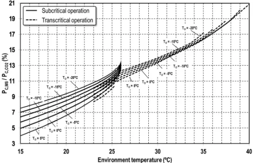
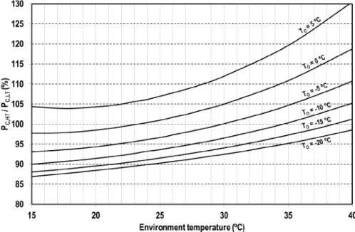
(9) Appl. Sci. 2017, 7, 955. 9 of 22. Finally, the ratio between the power consumption of the auxiliary cycle (R1234yf) and the main compressor (CO2 ), Equation (10), are represented in percentage for the optimum operating conditions in Figure 8. For the considered range, the needed power consumption of the auxiliary compressor ranges from 4% at an evaporation of 5 ◦ C and environment temperature of 15 ◦ C to 21% approximately for 5 ◦ C at 40 ◦ C. The most important observation is that sizing the auxiliary compressor for high Figure Optimum subcooling of the MS environment temperatures will 7. cover the operation indegrees transcritical andcycle. subcritical without problems.. Figure 8. Ratio Ratio of of compressor’s compressor’s power power consumptions consumptions of of the the MS MS cycle. cycle. Figure. 3.2. Operating Operating Conditions Conditions of of the the Cascade Cycle For the cascade cascadecycle, cycle,the theparameter parameter that must optimized is intermediate the intermediate temperature that must be be optimized is the temperature level level (T I ), the condensing temperature of CO 2 (T K,L ) being considered in this case for its (TI ), the condensing temperature of CO2 (TK,L ) being considered in this case for its representation. representation. As of mentioned, exitcondenser of CO2 cascade condenser is in saturation, no subcooling As mentioned, exit CO2 cascade is in saturation, no subcooling is considered, because is it considered, because it provides Figure of 9 the presents evolution of the provides lower efficiency results. lower Figureefficiency 9 presentsresults. the evolution overallthe COP of the cascade overall the cascade solution evaporation of 0 °C temperatures. for all the considered solutionCOP for anofevaporation level of 0 ◦ Cfor for an all the consideredlevel environment Limits of environment temperatures. Limits ofover variation of TK,L arepressure any temperature over the temperature evaporating variation of TK,L are any temperature the evaporating up to a condensing pressure a condensing temperature K below the◦ C) environment temperature (if In TenvFigure < 25.978 5 K belowup thetoenvironment temperature (if 5Tenv < 25.978 or the critical temperature. 9 it °C) or theclear critical Figure 9 it becomes clear anemphasis optimumisTdone K,L temperature exists. becomes thattemperature. an optimumIn TK,L temperature exists. Nothat more because different No morestudied emphasis is done authors studied it in detail [29,30]. COP values at the authors it in detailbecause [29,30]. different COP values at the optimum TK,L are presented in Figure 10. optimum T K,L are presented in Figure 10. In contrast to the COP evolutions of the MS cycle, it needs In contrast to the COP evolutions of the MS cycle, it needs to be highlighted that the reduction to highlighted that the reduction COP of cascade systems due to variations of environment of be COP of cascade systems due to of variations of the environment temperature is the smoother, being temperature smoother, these of systems less sensitive to variations of environmental these systemsisless sensitive being to variations environmental conditions, as previously mentioned by conditions, previously mentioned Llopisofetthe al.cascade [14]. Also, to compare of the cascade Llopis et al.as [14]. Also, to compare theby design system, the ratiothe of design the high-temperature and low-temperature power consumption are presented in Figure 11. In this case, the power consumption of the high-temperature compressor inside the evaluated range is of the same order of magnitude as that of the CO2 cycle. With a design of the plant as cascade, it could operate with the MS cycle but not the other way round..

(10) Appl. Appl. Sci. Sci. 2017, 2017, 7, 7, 955 955. 10 10 of of 22 22. system, system, the the ratio ratio of of the the high‐temperature high‐temperature and and low‐temperature low‐temperature power power consumption consumption are are presented presented in in Figure 11. In this case, the power consumption of the high‐temperature compressor inside the Figure 11. In this case, the power consumption of the high‐temperature compressor inside the evaluated range evaluated range is is of of the the same same order order of of magnitude magnitude as as that that of of the the CO CO22 cycle. cycle. With With aa design design of of the the10plant plant Appl. Sci. 2017, 7, 955 of 22 as as cascade, cascade, it it could could operate operate with with the the MS MS cycle cycle but but not not the the other other way way round. round.. Figure on the low‐temperature condensing temperature of system. (T Figure 9. 9. COP COPdependence dependence low-temperature condensing temperature of cascade system. Figure 9. COP dependence onon thethe low‐temperature condensing temperature of cascade cascade system. (Too == ◦ 00(T°C). o = 0 C). °C).. Figure 10. COP COP of the the cascade cycle cycle at optimum optimum conditions. Figure Figure 10. 10. COP of of the cascade cascade cycle at at optimum conditions. conditions..

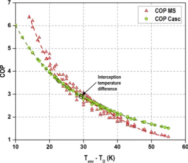
(11) Appl. Sci. 2017, 7, 955 Appl. Sci. 2017, 7, 955. 11 of 22 11 of 22. Figure Ratio of of compressor’s compressor’s power power consumptions consumptions of of the the cascade cascade cycle. Figure 11. 11. Ratio cycle.. 4. Discussion of Results The optimum both cycles were analyzed in Section 3. As3.mentioned, both optimumoperating operatingconditions conditionsofof both cycles were analyzed in Section As mentioned, refrigeration cycles cycles respond to the same scheme operation (Figure 1) and may1) beand ablemay to operate with both refrigeration respond to the same of scheme of operation (Figure be able to one scheme thescheme other ifor some components the plant are However, in practice, only operate withorone the other if someofcomponents ofover-sized. the plant are over‐sized. However, in one design of the is implemented to economicdue reasons, for example: if the is designed practice, only oneplant design of the plant isdue implemented to economic reasons, forplant example: if the to be operated in to both theincascade/subcooler heat exchanger must be sized asmust cascade heat plant is designed be modes operated both modes the cascade/subcooler heat exchanger be sized exchanger, whileexchanger, if it were designed be operated the subcooler would be size reduced. as cascade heat while if ittowere designedastoMS be cycle operated as MS cycle the subcooler would The same happens forsame the gas-cooler, a gas-cooler of a cascade systemofisasmaller that is of smaller the MS be size reduced. The happens for the gas‐cooler, a gas‐cooler cascadethan system cycle. Furthermore, optimum COP results of both solutions are compared (Figures 6are andcompared 10) it can than that of the MSifcycle. Furthermore, if optimum COP results of both solutions be seen that the MS the best at cycle low environment temperatures cascade at (Figures 6 and 10) cycle it canoffers be seen that results the MS offers the best results at and lowthe environment temperatures and the cascade at high temperatures. Thus,the this section is offered devotedbytoboth compare the high temperatures. Thus, this section is devoted to compare COP values solutions. COP the values offered byoperating both solutions. range each is First, recommended range ofFirst, each the cyclerecommended is analyzed in operating terms of COP, andofthen thecycle results analyzed in terms COP, and thenregions the results are through translated the different regions of are translated to theof different climatic of Spain thetocomputation of climatic the average annual Spain The through the computation of the average annual COP. Thewould objective is to obtain conclusions COP. objective is to obtain conclusions about which system be more recommended for system level would moreclimatic recommended aabout givenwhich evaporating in be a given region. for a given evaporating level in a given climatic region. 4.1. Recommended Operating Conditions. 4.1. Recommended Operating COP values offered by Conditions both cycle configurations are merged in Figure 12, where the COP value at each evaporating and environment corresponds the best system. it can be COP values offered by both cycle level configurations areto merged in performing Figure 12, where theAs COP value observed, the cascade system gets over the MS solution at high environment temperatures and low at each evaporating and environment level corresponds to the best performing system. As it can be evaporating In system fact, thegets environment temperature a given evaporating level thatand defines observed, thelevels. cascade over the MS solution atfor high environment temperatures low the border oflevels. both systems is expressed by Equation (11),for which wasevaporating fitted from level the results of the evaporating In fact, the environment temperature a given that defines models. At of environment temperatures above the value(11), given by Equation (11), thethe cascade solution the border both systems is expressed by Equation which was fitted from results of the operates with highest COP. Also, the optimum operation of the (11), MS cycle are depicted in models. At environment temperatures above themodes value of given by Equation the cascade solution ◦ C and that defined Figure 12. The operating conditions between an environment temperature of 25.3 operates with highest COP. Also, the optimum modes of operation of the MS cycle are depicted in by Equation (11)operating will be inconditions transcritical conditions, whereas all lower environment the best Figure 12. The between an environment temperature of 25.3levels °C and that performing cycle will(11) be in subcritical. As it is observed in Figure 12,all thelower environmental conditions at defined by Equation will be in transcritical conditions, whereas environment levels the which the plant would be operated in transcritical are very narrow, which means that the correct design best performing cycle will be in subcritical. As it is observed in Figure 12, the environmental of the first CO exchanger wouldbebeoperated as condenser. In an attempt to summarize all the results of 2 heat the conditions at which plant would in transcritical are very narrow, which means that Figure 12, the COP dependence cycles versus the temperature difference In between the cold the correct design of the first of COboth 2 heat exchanger would be as condenser. an attempt to and hot sources, Equation (12), is presented in Figure 13. Data used in Figure 13 correspond to all the summarize all the results of Figure 12, the COP dependence of both cycles versus the temperature. difference between the cold and hot sources, Equation (12), is presented in Figure 13. Data used in Figure 13 correspond to all the calculated points to represent Figure 12. It can be observed that the.

(12) Appl. Appl. Sci. 2017, 7, 955. 12 of 22. MS cycle offers highest COP values at reduced temperature lifts and the cascade the other way calculated Figure 12.liftIt of can28.5 be observed that the MS cycle offers COPto values round. Thepoints limit to is represent at a temperature K approximately. However, it ishighest important note Appl. Sci.temperature 2017, 7, 955 12 of 22lift of at reduced lifts and the cascade the other way round. The limit is at a temperature that the difference between the COP values of the MS cycle regards the cascade are higher at low 28.5 K approximately. However, it isbetween important to note thattemperature the difference between the COP values temperature that the difference them at high Those MS cyclelifts offers highest COP values at reduced temperature lifts and thelifts. cascade theCOP otherdifferences way of the MS cycle regards the cascade are higher at low temperature lifts that the difference between will round. condition of the system along different environment therefore a The the limitoperation is at a temperature lift of 28.5 K approximately. However, temperatures, it is important to note them at high temperature lifts. Those COP differences will condition the operation of the system along climatic evaluation would be needed to compare both cycles. That is discussed in Section 4.2. that the difference between the COP values of the MS cycle regards the cascade are higher at low different environment temperatures, climatic evaluation would needed compare both temperature lifts that the differencetherefore between athem at high temperature lifts.be Those COPto differences (11) T 25.95 0.4T cycles. That is discussed in Section 4.2. will condition the operation of the system along different environment temperatures, therefore a climatic evaluation would be needed to compare ∆T Tboth cycles. T That is discussed in Section 4.2.. Tenv = 25.95 + 0.4To T. 25.95. 0.4T. ∆T ∆T= T Tenv −TTo. (11) (12). Figure 12.12. Best performing cycle forthe thedifferent different operating conditions. Figure Best performing cycle cycle for operating conditions. Figure 12. Best performing for the different operating conditions.. Figure 13. COP dependence on cold and hot sink temperature lift. MS and cascade cycles.. Figure 13. 13. COP COP dependence dependence on on cold cold and and hot hot sink sink temperature temperature lift. lift. MS MS and and cascade cascade cycles. cycles. Figure. (12) (11) (12).

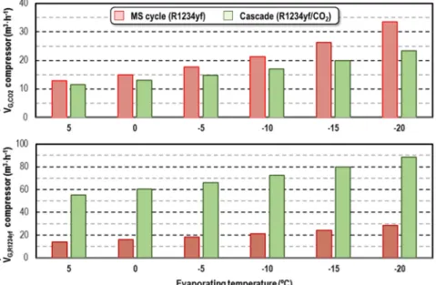
(13) Appl. Sci. 2017, 7, 955 Appl. Sci. 2017, 7, 955. 13 of 22 13 of 22. Although Although in in Figure Figure 12 12 it it seems seems that that aa smooth smooth transition transition between between the the MS MS and and the the cascade cascade cycle cycle would thethe cycle is sized to operate in both configurations. To would be be possible, possible,ititwill willonly onlyhappen happenwhen when cycle is sized to operate in both configurations. illustrate this reasoning, the compressor’s displacements for the low and high temperature cycles for To illustrate this reasoning, the compressor’s displacements for the low and high temperature cycles both configurations are are presented in Figure 14.14. Those data correspond to to thethe displacements forfor a for both configurations presented in Figure Those data correspond displacements refrigeration cooling capacity capacitydesigned designedfor forananenvironment environment temperature of ◦30 a refrigerationplant plantwith with50 50kW kW of of cooling temperature of 30 C. °C. It can be observed that the differences of the CO 2 compressor are not much significant between It can be observed that the differences of the CO2 compressor are not much significant between both both cycles’ solutions, but the compressor the cascade cycle would be300% up tohigher 300% than higher than that cycles’ solutions, but the compressor of the of cascade cycle would be up to that needed needed for the MS cycle. If the plant is sized to be operated as MS cycle, its operation as cascade for the MS cycle. If the plant is sized to be operated as MS cycle, its operation as cascade would not be would be possible of theand, compressors, and,evaluated, although because not evaluated, because the size possiblenot because of the because compressors, although not of the size of theofsubcooler of thethe subcooler and the gas‐cooler. and gas-cooler.. Figure 14. Compressor’s displacements of a plant with 50 kW capacity at an environment at 30 ◦ C. Figure 14. Compressor’s displacements of a plant with 50 kW capacity at an environment at 30 °C.. 4.2. Operation Operation in in Different Different Climate Climate Conditions Conditions 4.2. As mentioned mentioned by by Minetto Minetto et et al. al. [31], [31], the the superiority superiority of of one one refrigeration refrigeration system system regards regards another another As in terms of energy efficiency must be discussed with reference to the climatic conditions of the the in terms of energy efficiency must be discussed with reference to the climatic conditions of installation site and the characteristics of cooling profile. In agreement with them, and in order installation site and the characteristics of cooling profile. In agreement with them, and in order to to obtain conclusions about the performance the MS configuration cycle configuration the cascade obtain conclusions about the performance of theofMS cycle regardsregards the cascade design, design, in this subsection an evaluation of the systems at different climate conditions is reported. in this subsection an evaluation of the systems at different climate conditions is reported. In this In this case, a climatic evaluation wasusing madethe using BIN temperature methodology the case, a climatic evaluation was made BINthe temperature methodology [32] with[32] thewith Energy Energy Plus meteorological data (https://energyplus.net/weather) for different locations in Spain. Plus meteorological data (https://energyplus.net/weather) for different locations in Spain. This This methodology groups the number of annual hours in which a certain temperature was recorded, methodology groups the number of annual hours in which a certain temperature was recorded, allowing an an accurate accurate representation representation of of the the annual annual climate. allowing climate. In fact, the energy performance of the systems wasevaluated evaluated twelve climatic regions In fact, the energy performance of the systems was forfor thethe twelve climatic regions of of Spain [33], Table 1, covering cold, mild and warm climates, using 20 temperature Spain [33], Table 1, covering cold, mild and warm climates, using 20 temperature BINs from −3 BINs to 33 from 3 to 33 ◦temperature. C of dry bulb temperature. Fortwo the simplified evaluation,cooling two simplified cooling profiles °C of − dry bulb For the evaluation, load profiles wereload considered. were considered. Representing air-conditioning (AC) applications, no cooling load was considered Representing air‐conditioning (AC) applications, no cooling load was considered below 21 °C, a linear ◦ C and below 21 ◦ C,on a the linear dependence ontemperatures the cooling load from temperatures up 29 to °C 29 on. dependence cooling load from above 21 up to 29 °C andabove 100%21 from For ◦ ◦ C, 100% from 29 C on. For commercial applications a constant value of 50% of cooling load up to 23 commercial applications a constant value of 50% of cooling load up to 23 °C, linear dependence from ◦ linear and 100% 31 ºC Cooling load 1. profiles are detailed in 23 to 31dependence °C and 100%from from23 31toºC31 on.CCooling loadfrom profiles areon. detailed in Table Table 1..

(14) Appl. Sci. 2017, 7, 955. 14 of 22. Table 1. Reference Spanish cities for the evaluation of the systems. Climatic regions, temperature BINs, hours of operation and cooling load profiles. City. León. Pamplona. Teruel. Albacete. La Coruña. Barcelona. Granada. Toledo. Spanish climatic region Average annual temperature (◦ C). E1 10.79. D1 12.22. D2 11.55. D3 13.51. C1 14.14. C2 15.37. C3 14.88. C4 15.57. Temperature BIN. AC cooling load (%). Commercial cooling load (%). <−3 −3 to −1 −1 to 1 1 to 3 3 to 5 5 to 7 7 to 9 9 to 11 11 to 13 13 to 15 15 to 17 17 to 19 19 to 21 21 to 23 23 to 25 25 to 27 27 to 29 29 to 31 31 to 33 >33. 0 0 0 0 0 0 0 0 0 0 0 0 0 0.2 0.4 0.6 0.8 1 1 1. 0.5 0.5 0.5 0.5 0.5 0.5 0.5 0.5 0.5 0.5 0.5 0.5 0.5 0.5 0.6 0.7 0.8 0.9 1 1. Castellón de la Plana B3 16.74. Sevilla. Málaga. Almería. B4 18.25. A3 17.99. A4 18.54. 0 0 0 0 0 62 754 846 785 789 858 841 1008 581 581 523 275 243 304 310. 0 0 0 0 0 0 62 996 1055 941 884 1061 1002 919 738 397 426 279 0 0. 0 0 0 0 0 0 0 810 943 933 975 1094 851 1068 800 488 458 340 0 0. Annual hours inside the temperature BIN 0 0 248 990 936 847 915 818 943 826 552 492 244 304 304 155 186 0 0 0. 0 0 0 341 962 1114 819 884 846 944 765 615 430 274 304 276 186 0 0 0. 0 0 391 878 875 633 887 734 751 855 733 522 430 213 244 273 217 124 0 0. 0 0 0 633 847 817 571 981 604 756 669 705 583 339 306 273 304 124 217 31. 0 0 0 0 0 0 537 1697 1364 1553 1556 950 673 430 0 0 0 0 0 0. 0 0 0 0 0 540 909 1057 819 1063 824 817 1046 613 518 337 217 0 0 0. 0 0 0 248 692 843 571 827 668 851 814 795 612 307 461 214 243 273 124 217. 0 0 0 155 602 663 876 663 949 572 638 578 764 615 431 275 183 393 155 248. 0 0 0 0 0 124 903 968 813 854 943 909 976 800 552 394 338 186 0 0.

(15) Appl. Sci. 2017, 2017, 7, 955. 15 of 22. Using the meteorological data of dry‐bulb temperature, an averaged COP value for both cycle Using the meteorological dry-bulb (13). temperature, an averaged valueoffor both cycle configurations was evaluated data usingofEquation Where COP (Tenv,i) is COP the COP each system configurations was evaluated using Equation (13). Where COP (T ) is the COP of each system evaluated at the average temperature of the ‘i’ temperature BIN, env,i NHi is the number of hours of evaluated at the average temperature of the ‘i’ temperature BIN, NH the number of hours of i isinside operation inside the ‘i’ temperature BIN and FQi the cooling load fraction the ‘i’ temperature operation inside the ‘i’ temperature BIN and FQ the cooling load fraction inside the ‘i’ temperature BIN. i BIN.. COP. ∑. COP NH) × NH FQi × FQi ] ∑nbin , (Tenv,i i=T 1 [COP nbin NHi × FQi ) ∑i=1 (FQ ∑ NH. COP =. (3). (13). Averaged COP values for both refrigeration systems, for the different climatic regions using the Averaged COP values for both refrigeration systems, for the different climatic regions using cooling load profiles detailed in Table 1, are summarized in Table 2. Regarding AC application (To = the cooling load profiles detailed in Table 1, are summarized in Table 2. Regarding AC application 5 °C), it can be seen that the MS cycle over performs the cascade configuration for all the climatic (To = 5 ◦ C), it can be seen that the MS cycle over performs the cascade configuration for all the climatic regions except for the D3, C3, C4 and B4, that are regions with high environment temperatures regions except for the D3, C3, C4 and B4, that are regions with high environment temperatures during during summer, where both configuration perform similar. Regarding the general application, for summer, where both configuration perform similar. Regarding the general application, for evaporating evaporating temperatures from 0 to −20 °C, the MS cycle also presents highest performance for all temperatures from 0 to −20 ◦ C, the MS cycle also presents highest performance for all the climatic the climatic regions up to an evaporating level of −10 °C. At −15 °C both solutions perform similar regions up to an evaporating level of −10 ◦ C. At −15 ◦ C both solutions perform similar and for and ◦for −20 °C the cascade solution is the best performing. The differences between both −20 C the cascade solution is the best performing. The differences between both refrigeration systems refrigeration systems for the different climate conditions and the different evaporating levels and for the different climate conditions and the different evaporating levels and cooling load profiles cooling load profiles are represented in Figure 15 as percentage variation from the MS cycle COP are represented in Figure 15 as percentage variation from the MS cycle COP values, according to values, according to Equation (14). Values of Equation (14) represent the average annual COP Equation (14). Values of Equation (14) represent the average annual COP advantage of the MS cycle advantage of the MS cycle regard the cascade cycle. It can be observed that the MS cycle is regard the cascade cycle. It can be observed that the MS cycle is recommended from an energy point of recommended from an energy point of view for any evaporating level higher or equal to −10 °C, both view for any evaporating level higher or equal to −10 ◦ C, both systems similar perform at −15 ◦ C and systems similar perform at −15 °C and the cascade should be recommended for the temperature level the cascade should be recommended for the temperature level of −20 ◦ C. of −20 °C. COP − COPcasc ∆COP × 100 (14) ) = COPMS COP 100 ∆COP(%% (14) COP COP casc. Figure 15. variation of MS vs. thevs. cascade system at different Figure 15.COP COPpercentage percentage variation of cycle MS cycle the cascade system at climatic differentcondition. climatic condition..

(16) Appl. Sci. 2017, 7, 955. 16 of 22. Table 2. Averaged annual COP of cascade and MS cycles for Spanish Climate Regions. Climatic Region. E1. D1. Cascade cycle annual averaged COP To = 5 ◦ C (AC) 3.74 3.72 To = 0 ◦ C 4.51 4.45 To = − 5 ◦ C 3.75 3.70 To = −10 ◦ C 3.18 3.14 To = −15 ◦ C 2.73 2.70 To = −20 ◦ C 2.37 2.35 MS cycle annual averaged COP To = 5 ◦ C (AC) 3.92 3.88 To = 0 ◦ C 5.65 5.52 To = − 5 ◦ C 4.38 4.29 To = −10 ◦ C 3.50 3.44 To = −15 ◦ C 2.86 2.81 To = −20 ◦ C 2.36 2.32 Climatic region E1 D1 Cascade cycle annual averaged COP To = 5 ◦ C (AC) 3.74 3.72 To = 0 ◦ C 4.51 4.45 To = − 5 ◦ C 3.75 3.70 To = −10 ◦ C 3.18 3.14 To = −15 ◦ C 2.73 2.70 To = −20 ◦ C 2.37 2.35 MS cycle annual averaged COP To = 5 ◦ C (AC) 3.92 3.88 To = 0 ◦ C 5.65 5.52 To = − 5 ◦ C 4.38 4.29 To = −10 ◦ C 3.50 3.44 To = −15 ◦ C 2.86 2.81 To = −20 ◦ C 2.36 2.32. D2. D3. C1. C2. C3. C4. B3. B4. A3. A4. 3.57 4.42 3.68 3.12 2.69 2.33. 3.41 4.23 3.54 3.01 2.60 2.26. 4.30 4.53 3.77 3.19 2.74 2.38. 3.79 4.26 3.56 3.03 2.61 2.27. 3.33 4.13 3.46 2.95 2.55 2.22. 3.33 4.04 3.39 2.90 2.51 2.18. 3.66 4.11 3.45 2.95 2.54 2.22. 3.34 3.87 3.26 2.80 2.42 2.12. 3.63 4.00 3.37 2.88 2.49 2.17. 3.63 3.94 3.32 2.84 2.46 2.15. 3.65 5.48 4.26 3.41 2.79 2.30 D2. 3.43 5.14 4.02 3.23 2.65 2.19 D3. 4.82 5.67 4.40 3.52 2.87 2.37 C1. 4.00 5.16 4.04 3.25 2.67 2.21 C2. 3.32 4.97 3.89 3.14 2.58 2.13 C3. 3.33 4.81 3.78 3.06 2.51 2.08 C4. 3.80 4.89 3.85 3.11 2.56 2.12 B3. 3.34 4.49 3.55 2.89 2.38 1.98 B4. 3.76 4.68 3.70 3.00 2.48 2.06 A3. 3.76 4.56 3.62 2.94 2.43 2.02 A4. 3.57 4.42 3.68 3.12 2.69 2.33. 3.41 4.23 3.54 3.01 2.60 2.26. 4.30 4.53 3.77 3.19 2.74 2.38. 3.79 4.26 3.56 3.03 2.61 2.27. 3.33 4.13 3.46 2.95 2.55 2.22. 3.33 4.04 3.39 2.90 2.51 2.18. 3.66 4.11 3.45 2.95 2.54 2.22. 3.34 3.87 3.26 2.80 2.42 2.12. 3.63 4.00 3.37 2.88 2.49 2.17. 3.63 3.94 3.32 2.84 2.46 2.15. 3.65 5.48 4.26 3.41 2.79 2.30. 3.43 5.14 4.02 3.23 2.65 2.19. 4.82 5.67 4.40 3.52 2.87 2.37. 4.00 5.16 4.04 3.25 2.67 2.21. 3.32 4.97 3.89 3.14 2.58 2.13. 3.33 4.81 3.78 3.06 2.51 2.08. 3.80 4.89 3.85 3.11 2.56 2.12. 3.34 4.49 3.55 2.89 2.38 1.98. 3.76 4.68 3.70 3.00 2.48 2.06. 3.76 4.56 3.62 2.94 2.43 2.02.

(17) Appl. Sci. 2017, 7, 955 Appl. Sci. 2017, 7, 955. 17 of 22 17 of 22. As previously mentioned, both refrigeration cycle designs could be implemented in a system As previously mentioned, refrigeration cycle could be implemented a system and if if some of the components areboth oversized, mainly the designs high temperature compressor,insubcooler some of the components are oversized, mainly the done. high temperature subcooler and gas-cooler/condenser, although it is not commonly Nonetheless,compressor, if only one cycle of operation gas‐cooler/condenser, although it is not commonly done. Nonetheless, if only one cycle of operation is selected, it is important to quantify what would be its overall performance regards a plant with is selected, it is important to quantify what would be its overall performance regards a plant with possibility to operate as cascade or as MS cycle, that would be the plant that will offer the best possibility to operate as cascade or as MS cycle, that would be the plant that will offer the best average annual COP values. To quantify the differences of the individual systems, their average average annual COP values. To quantify the differences of the individual systems, their average annual COP values according to Equation (13) were compared to the ones obtained by an ideal annual COP values according to Equation (13) were compared to the ones obtained by an ideal refrigeration system with COP values equal to the maximum COP values of the MS or the cascade refrigeration system with COP values equal to the maximum COP values of the MS or the cascade system. Percentage annual COP deviations regards the ideal system are specified in Table 3 for system. Percentage annual COP deviations regards the ideal system are specified in Table 3 for the the different Spanish climate regions, and represented for two representative cases in Figure 16, which different Spanish climate regions, and represented for two representative cases in Figure 16, which correspond to the operation at −5 ◦ C and −20 ◦ C of evaporating temperature. As it can be observed, correspond to the operation at −5 °C and −20 °C of evaporating temperature. As it can be observed, any individual system has reductions of annual COP values regards the optimum or best system, any individual system has reductions of annual COP values regards the optimum or best system, since in some hours of the year the other solution would be more performing. That occurs for all since in some hours of the year the other solution would be more performing. That occurs for all the the climatic regions and evaporating levels except for the climatic region C1 with evaporating levels climatic regions and evaporating levels except for the climatic region C1 with evaporating levels from 5 to −5 ◦ C. In general, for all the climatic regions, the system that better performs is the MS cycle from 5 to −5 °C. In general, for all the climatic regions, the system that better performs is the MS cycle configuration,with withannual annualdeviations deviations from best system to at 5%evaporating at evaporating higher configuration, from thethe best system up up to 5% levelslevels higher or ◦ C. On the other side, if the considered evaporating level is −20 ◦ C, the solution or equal than − 15 equal than −15 °C. On the other side, if the considered evaporating level is −20 °C, the solution with withdeviation less deviation from thesystem ideal system is the cascade, however, it is important to note the MS less from the ideal is the cascade, however, it is important to note that the that MS cycle cycle willdeviations have deviations lower 5% regards idealfor system for all the regions climaticexcept regions will have lower than 5%than regards the idealthe system all the climatic forexcept the for the C4, B4, A3 and A4. That indicates that although the MS cycle does not reach the performance C4, B4, A3 and A4. That indicates that although the MS cycle does not reach the performance of the of the cascade −average 20 ◦ C, its average annual performance would be good for all cascade solutionsolution at −20 °C,atits annual performance would be good enough for allenough the climatic the climatic conditions without large reductions of efficiency. This solution will avoid the over conditions without large reductions of efficiency. This solution will avoid the over sizing of sizing the of the and plant, andallow thus,toallow to operate with acost lower cost plant. plant, thus, operate with a lower plant.. Figure averageannual annualCOP COPdeviations deviations cascade cycles regards thesystem. best Figure 16. 16. Percentage average of of MSMS andand cascade cycles regards the best system..

(18) Appl. Sci. 2017, 7, 955. 18 of 22. Table 3. Percentage deviation of annual COP values of MS and cascade cycles regards the best system. Climatic Region. E1. Cascade cycle −4.7 −20.2 −14.6 −9.7 −5.5 −1.4 MS cycle To = 5 ◦ C (AC) −0.2 To = 0 ◦ C −0.1 To = − 5 ◦ C −0.3 To = −10 ◦ C −0.6 To = −15 ◦ C −1.1 To = −20 ◦ C −1.9. To = 5 ◦ C (AC) To = 0 ◦ C To = − 5 ◦ C To = −10 ◦ C To = −15 ◦ C To = −20 ◦ C. D1. D2. D3. C1. C2. C3. C4. B3. B4. A3. A4. −4.3 −19.6 −14.1 −9.3 −5.2 −1.3. −3.1 −19.6 −14.1 −9.3 −5.2 −1.3. −2.6 −18.2 −12.9 −8.4 −4.6 −1.1. −10.9 −20.0 −14.3 −9.3 −5.0 −1.1. −5.2 −17.5 −12.3 −7.8 −4.1 −1.0. −2.5 −17.4 −12.3 −7.9 −4.2 −1.0. −2.8 −16.6 −11.6 −7.4 −4.0 −1.0. −4.3 −16.2 −11.2 −6.9 −3.6 −0.8. −2.7 −14.6 −10.0 −6.1 −3.1 −0.7. −4.2 −14.9 −10.1 −6.2 −3.1 −0.7. −4.1 −14.2 −9.5 −5.7 −2.8 −0.6. −0.2 −0.1 −0.3 −0.7 −1.3 −2.4. −0.8 −0.2 −0.5 −0.9 −1.5 −2.6. −2.0 −0.5 −1.0 −1.6 −2.5 −4.0. 0.0 0.0 0.0 −0.1 −0.4 −1.5. −0.1 −0.1 −0.5 −1.0 −2.0 −3.8. −2.7 −0.7 −1.3 −2.0 −3.1 −4.8. −2.8 −0.9 −1.5 −2.4 −3.7 −5.6. −0.7 −0.4 −0.8 −1.6 −2.9 −5.0. −2.7 −1.1 −1.9 −3.1 −4.7 −7.1. −0.8 −0.5 −1.1 −2.1 −3.6 −6.1. −0.8 −0.6 −1.3 −2.4 −4.1 −6.7.

(19) Appl. Sci. 2017, 7, 955. 19 of 22. 5. Conclusions This communication analyzes two modes of operation of a CO2 -based two-stage refrigeration cycle with equivalent design that can be operated as cascade refrigeration system or as a CO2 refrigeration plant with dedicated mechanical subcooling system. Both schemes are being considered now to spread the use of CO2 in medium and warm regions of the planet for medium temperature applications. Using relations of the overall efficiency of compressors, adjusted from experimental data of a semi-hermetic CO2 and a semi-hermetic R1234yf compressors, a simplified model of both cycles was developed. With the thermodynamic models, the optimum operating conditions of each refrigeration cycle, covering evaporating temperatures from −20 to 5 ◦ C and environment temperatures from 15 to 40 ◦ C, were determined. Then, by merging the COP values of each refrigeration solution, the external conditions at which each refrigeration solution is the best performing were established. Furthermore, the analysis was translated for the different climatic regions of Spain to compare the systems. Regarding the CO2 refrigeration cycle with mechanical subcooling, it was concluded that the environment temperature that will limit the operation in subcritical or transcritical is 25.3 ◦ C, thus the design of the gas-cooler would be always as condenser, since the region at which this system will operate in transcritical is very narrow. Furthermore, the optimum subcooling degree results higher at lowest evaporating levels and high environment levels. Nonetheless, the maximum ratio of power consumption of the mechanical subcooling compressor will not exceed from 21% of the power consumption of the CO2 compressor. It was concluded that the cascade configuration using CO2 as low temperature refrigerant will have highest performance than the MS cycle when the temperature lift between the cold and heat sources is higher than 28.5 K. However, in this case the power consumption of the high-temperature cycle will be even higher than the power consumption of the CO2 rack. The analysis was extended to the different climatic regions of Spain using a based temperature-BIN methodology. It was calculated that the MS cycle would offer highest energy efficiencies in overall-year operation than the cascade solution for evaporating levels below −15 ◦ C, including the air-conditioning application. However, at the evaporating level of −20 ◦ C the cascade solution will over perform the MS cycle. Also, the individual systems were compared to an ideal refrigeration cycle that could be operated as CO2 with mechanical subcooling or as cascade at any climatic condition, which is called the best system. The average annual COP of each individual system was compared with the best system. It was observed that the MS cycle will have annual reductions of efficiency up to 5% at evaporating levels higher or equal than −15 ◦ C, and also reductions below 5% at the evaporating level of −20 ◦ C except for 4 climatic regions of Spain. As general conclusion of this work, it can be affirmed that if this cycle configuration is sized as cascade or as a single-stage cycle with mechanical subcooling, the configuration that will offer the best performing levels at the analyzed conditions would be the CO2 refrigeration cycle with mechanical subcooling. Acknowledgments: The authors gratefully acknowledge the Spanish Ministry of Economy and Competitiveness (project ENE2014-53760-R.7) for financing this research work. Author Contributions: R.L. suggested the idea and conceived the calculation models. R.L. and L.N.-A. carried out the simulations and analyzed the data; D.S. and R.C. checked the calculations. R.L. and L.N.-A. wrote the paper and J.C.-G. contributed to the correction of the paper. Conflicts of Interest: The authors declare no conflict of interest.. Nomenclature Casc COP FQ GWP HX. cascade cycle with CO2 as low temperature refrigerant coefficient of performance cooling load fraction inside a temperature BIN Global warming potential heat exchanger.

(20) Appl. Sci. 2017, 7, 955. h NH nbin MS . m P PC .. QO SUB T t TEWI . VG GREEK SYMBOLS ηG ∆ ε SUBSCRIPTS CO2 crit env gc H high I K L MS O R1234yf sat. 20 of 22. specific enthalpy, kJ·kg−1 number of hours inside a temperature BIN number of temperature bins CO2 cycle with mechanical subcooling mass flow rate, kg·s−1 pressure, bar compressor power consumption, kW cooling capacity, kW degree of subcooling at the subcooler, K temperature, ◦ C compression ratio total equivalent warming impact compressor displacement, m3 ·h−1 overall compressor efficiency increment heat exchanger efficiency referring to CO2 cycle critical point environment gas-cooler hot sink refers to pressure at gas-cooler and subcooler or cascade heat exchanger intermediate temperature level condensing level cold source, low temperature cycle referring to the dedicated mechanical subcooling cycle evaporating level referring to the R1234yf cycle saturation. References and Notes 1. 2. 3. 4. 5. 6. 7. 8. 9.. European Commission. Regulation (EU) No 517/2014 of the European Parliament and of the Council of 16 April 2014 on Fluorinated Greenhouse Gases and Repealing Regulation (EC) No 842/2006; 2014. Hafner, A.; Hemmingsen, A.K. R744 refrigeration technologies for supermarkets in warm climates. In Proceedings of the 24th IIR International Congress of Refrigeration, Yokohama, Japan, 16–22 August 2015. Kim, M.H.; Pettersen, J.; Bullard, C.W. Fundamental process and system design issues in CO2 vapor compression systems. Prog. Energy Combust. Sci. 2004, 30, 119–174. [CrossRef] Jia, X.; Zhang, B.; Pu, L.; Guo, B.; Peng, X. Improved rotary vane expander for trans-critical CO2 cycle by introducing high-pressure gas into the vane slots. Int. J. Refrig. 2011, 34, 732–741. [CrossRef] Hu, J.; Li, M.; Zhao, L.; Xia, B.; Ma, L. Improvement and experimental research of CO2 two-rolling piston expander. Energy 2015, 93, 2199–2207. [CrossRef] Elbel, S.; Lawrence, N. Review of recent developments in advanced ejector technology. Int. J. Refrig. 2016, 62, 1–18. [CrossRef] Hafner, A.; Banasiak, K.; Herdlitschka, T.; Fredslund, K.; Girotto, S.; Haida, M.; Smolka, J. ‘R744 Ejector System Case: Italian Supermarket, Spiazzo’, in Refrigeration Science and Technology. 2016, pp. 471–478. Lawrence, N.; Elbel, S. ‘Experimental Study on Control Methods for Transcritical Co2 Two-Phase Ejector Systems at Off-Design Conditions’, in Refrigeration Science and Technology. 2016, pp. 511–518. Karampour, M.; Sawalha, S. ‘Integration of Heating and Air Conditioning into a Co2 Trans-Critical Booster System with Parallel Compression Part I: Evaluation of Key Operating Parameters Using Field Measurements’, in Refrigeration Science and Technology. 2016, pp. 323–331..

(21) Appl. Sci. 2017, 7, 955. 10. 11.. 12. 13. 14.. 15. 16. 17. 18.. 19.. 20. 21. 22. 23.. 24. 25. 26. 27.. 28. 29. 30. 31.. 21 of 22. Aprea, C.; Greco, A.; Maiorino, A. The application of a desiccant wheel to increase the energetic performances of a transcritical cycle. Energy Convers. Manag. 2015, 89, 222–230. [CrossRef] Arora, A.; Singh, N.K.; Monga, S.; Kumar, O. Energy and exergy analysis of a combined transcritical CO2 compression refrigeration and single effect H2 O-LiBr vapour absorption system. Int. J. Exergy 2011, 9, 453–471. [CrossRef] Sanz-Kock, C.; Llopis, R.; Sánchez, D.; Cabello, R.; Torrella, E. Experimental evaluation of a R134a/CO2 cascade refrigeration plant. Appl. Therm. Eng. 2014, 73, 39–48. [CrossRef] Peñarrocha, I.; Llopis, R.; Tárrega, L.; Sánchez, D.; Cabello, R. A new approach to optimize the energy efficiency of CO2 transcritical refrigeration plants. Appl. Therm. Eng. 2014, 67, 137–146. [CrossRef] Llopis, R.; Sánchez, D.; Sanz-Kock, C.; Cabello, R.; Torrella, E. Energy and environmental comparison of two-stage solutions for commercial refrigeration at low temperature: Fluids and systems. Appl. Energy 2015, 138, 133–142. [CrossRef] Hafner, A.; Hemmingsen, A.K.; Van De Ven, A. ‘R744 Refrigeration System Configurations for Supermarkets in Warm Climates’, in Refrigeration Science and Technology. 2014, pp. 125–133. Gullo, P.; Elmegaard, B.; Cortella, G. Energy and environmental performance assessment of R744 booster supermarket refrigeration systems operating in warm climates. Int. J. Refrig. 2016, 64, 61–79. [CrossRef] Llopis, R.; Cabello, R.; Sánchez, D.; Torrella, E. Energy improvements of CO2 transcritical refrigeration cycles using dedicated mechanical subcooling. Int. J. Refrig. 2015, 55, 129–141. [CrossRef] Nebot-Andrés, L.; Llopis, R.; Sánchez, D.; Cabello, R. Experimental evaluation of a dedicated mechanical subcooling system in a CO2 transcritical refrigeration cycle, Refrigeration Science and Technology. 2016, pp. 965–972. Eikevik, T.M.; Bertelsen, S.; Haugsdal, S.; Tolstorebrov, I.; Jensen, S. ‘Co2 Refrigeration System with Integrated Propan Subcooler for Supermarkets in Warm Climate’, in Refrigeration Science and Technology. 2016, pp. 211–218. Ge, Y.T.; Tassou, S.A.; Santosa, I.D.; Tsamos, K. Design optimisation of CO2 gas cooler/condenser in a refrigeration system. Appl. Energy 2015, 160, 973–981. [CrossRef] Shao, L.L.; Zhang, C.L. Thermodynamic transition from subcritical to transcritical CO2 cycle. Int. J. Refrig. 2016, 64, 123–129. [CrossRef] Tsamos, K.M.; Ge, Y.T.; Santosa, I.D.M.C.; Tassou, S.A. Experimental investigation of gas cooler/condenser designs and effects on a CO2 booster system. Appl. Energy. 2017, 186, 470–479. [CrossRef] Sánchez, D.; Patiño, J.; Sanz-Kock, C.; Llopis, R.; Cabello, R.; Torrella, E. Energetic evaluation of a CO2 refrigeration plant working in supercritical and subcritical conditions. Appl. Therm. Eng. 2014, 66, 227–238. [CrossRef] Dopazo, J.A.; Fernández-Seara, J. Experimental evaluation of a cascade refrigeration system prototype with CO2 and NH3 for freezing process applications. Int. J. Refrig. 2011, 34, 257–267. [CrossRef] Aprea, C.; Greco, A.; Maiorino, A. An experimental investigation on the substitution of HFC134a with HFO1234YF in a domestic refrigerator. Appl. Therm. Eng. 2016, 106, 959–967. [CrossRef] Sánchez, D.; Torrella, E.; Cabello, R.; Llopis, R. Influence of the superheat associated to a semihermetic compressor of a transcritical CO2 refrigeration plant. Appl. Therm. Eng. 2010, 30, 302–309. [CrossRef] Llopis, R.; Nebot-Andrés, L.; Cabello, R.; Sánchez, D.; Catalán-Gil, J. Experimental evaluation of a CO2 transcritical refrigeration plant with dedicated mechanical subcooling. Int. J. Refrig. 2016, 69, 361–368. [CrossRef] Lemmon, E.W.; Huber, M.L.; McLinden, M.O. REFPROP, NIST Standard Reference Database 23, v.9.1; National Institute of Standards: Gaithersburg, MD, USA, 2013. Torrella, E.; Llopis, R.; Cabello, R. Experimental evaluation of the inter-stage conditions of a two-stage refrigeration cycle using a compound compressor. Int. J. Refrig. 2009, 32, 307–315. [CrossRef] Lee, T.S.; Liu, C.H.; Chen, T.W. Thermodynamic analysis of optimal condensing temperature of cascade-condenser in CO2 /NH3 cascade refrigeration systems. Int. J. Refrig. 2006, 29, 1100–1108. [CrossRef] Minetto, S.; Rossetti, A.; Girotto, S.; Marinetti, S. ‘Seasonal Performance of Supermarket Refrigeration Systems’, in Refrigeration Science and Technology. 2016, pp. 455–462..

(22) Appl. Sci. 2017, 7, 955. 32.. 33.. 22 of 22. The Australian Institute of Refrigeration, Air Conditioning and Heating (AIRAH), Methods of calculating Total Equivalent Warming Impact (TEWI) 2012. Available online: http://www.airah.org.au/imis15_prod/ Content_Files/BestPracticeGuides/Best_Practice_Tewi_June2012.pdf (accessed on 21 April 2017). Ministry of Housing, Royal Decree 314/2006, Spanish Technical Building Code. HE Enegy Saving Document. Available online: http://www.codigotecnico.org/ (accessed on 17 March 2017). © 2017 by the authors. Licensee MDPI, Basel, Switzerland. This article is an open access article distributed under the terms and conditions of the Creative Commons Attribution (CC BY) license (http://creativecommons.org/licenses/by/4.0/)..

(23)