Effectiveness of hedging with futures contracts

Texto completo

(1)DEGREE FINAL PROJECT. EFFECTIVENESS OF HEDGING WITH FUTURES CONTRACTS. Author: Moreno Munera, David E-mail: al258091@uji.es Tutor o supervisor: Nieto Soria, María Luisa Studies: Degree of Finances and Accounting University: Universitat Jaume I Year: 2015-2016.

(2) Abstract: This paper develops a model to hedging a portfolio of shares against the risk of the possible fall of the price through the use of futures on IBEX 35. We will evaluate the robustness of this coverage by subjecting it to various strategies and evaluating them in terms of efficiency. We will analyze your response hedging in different scenarios: 1) does not cover the stock portfolio, 2) cover the portfolio and maintain the future through expiration date and 3) cover the portfolio and cancel the futures position before the expiration date. With this we will obtain results with which we will be able to clarify a response of the efficiency of the hedging and correct use of which instrument is most effective to cover it.. Keywords: Hedging, Future market, Spot market, future contract, Underlying, Effectiveness, Base.. Resumen: En este trabajo se desarrolla un modelo para cubrir una cartera de acciones contra el riesgo de la posible caída del precio de las mismas mediante el uso de contratos de futuros sobre el IBEX 35. Valoraremos la robustez de ésta cobertura sometiéndola a varias estrategias y evaluándolas en términos de eficacia. Analizaremos cómo responde la cobertura en distintos escenarios: 1) No cubrimos la cartera de acciones, 2) Cubrimos la cartera y mantenemos el futuro hasta fecha de vencimiento y 3) Cubrimos la cartera y cancelamos la posición en futuros antes de la fecha de vencimiento. Con esto obtendremos unos resultados con los cuales podremos esclarecer una respuesta de la eficiencia de la cobertura y correcta utilización de qué instrumento es más eficaz para cubrirla.. Palabras Clave: Cobertura, Mercados de futuros, Mercado de contado, Contrato de futuro, Subyacente, Efectividad, Base.. 2.

(3) INDEX SECTION 1.. INTRODUCTION ...............................................................................................................7. 2.. FUTURE CONTRACTS AS HEDGING ..........................................................................9. 3.. 4.. 2.1.. ORIGIN OF FUTURES MARKETS...................................................................9. 2.2.. FUTURES IN SPAIN ...........................................................................................10. 2.3.. DIFERENCE BETWEEN FORWARD AND FUTURE ...............................11. 2.4.. FUTURES ON IBEX 35 ......................................................................................13. 2.5.. ADVANTAGES AND DISADVANTAGES OF USING A HEDGING .....14. CHOICE EFFICIENT PORTFOLIO ...............................................................................15 3.1.. CHOICE COMPANIES TO INVEST. .............................................................15. 3.2.. MODEL OF HARRY MARKOWITZ. ...............................................................16. 3.3.. CRITICISM OF THE MODEL “MEDIA -VARIANZA”. ................................25. HEDGING WITH FUTURES ..........................................................................................26 4.1.. DAILY PROFITABILITY PORTFOLIO ..........................................................26. 4.2.. CORRELATION COEFFICIENT ......................................................................27. 4.3.. REALIZATION OF HEDGING. ........................................................................33. 4.4.. HEDGING IN DATE OF EXPIRATION. ........................................................36. 4.5.. HEDGING A ONE WEEK BEFORE EXPIRATION ...................................39. 4.6.. COMPARISON OF BOTH HEDGINGS .........................................................41. 4.7. EFFECTIVENESS OF HEDGES. BECAUSE THE COVERAGE NOT IS PERFECT. ....................................................................................................................43. 5.. CONCLUSION .................................................................................................................45. 6.. BIBLIOGRAPHY .............................................................................................................47. 3.

(4) INDEX FIGURES Figure 1: "Schema futures markets" ............................................................................ 11 Figure 2: "Positions Spot market vs. Futures market" ................................................. 14 Figure 3: "IBEX 35 companies" .................................................................................... 16 Figure 4: "Efficient frontier Markowitz” ........................................................................ 17 Figure 5: “Quoted price companies” ............................................................................ 18 Figure 6: “Profitability companies” ............................................................................... 19 Figure 7: “Variances and covariances matrix” ............................................................ 19 Figure 8: “Profitability and Risk of the portfolio” .......................................................... 21 Figure 9: “Efficient frontier table” ................................................................................. 21 Figure 10: “Restrictions Solver” ................................................................................... 22 Figure 11: “Efficient frontier” ........................................................................................ 23 Figure 12: “Mixed Portfolio” ......................................................................................... 23 Figure 13: “Weight Shares” ......................................................................................... 24 Figure 14: “Portfolio composition” ............................................................................... 24 Figure 14: “Investment in Shares” ............................................................................... 26 Figure 15: “Graphic Portfolio Value” ............................................................................ 27 Figure 16: “Future conditions” ..................................................................................... 31 Figure 17: “Graphic Comparative Portfolio/Future” .................................................... 32 Figure 18: “Nominal future contract” ........................................................................... 33 Figure 19: “Hedging March 2015” ............................................................................... 34 Figure 20: “Hedging January 2016” ............................................................................ 34 Figure 21: “Hedging September 2015” ....................................................................... 35 Figure 22: “Hedging March 2015 before date expiration” ........................................... 36 Figure 23: “Summary Table Hedging in date expiration” ............................................ 37 Figure 24: “Graphic Hedging in date expiration” ......................................................... 38 Figure 25: “Summary Table Hedging a week before date expiration”......................... 39 Figure 26: “Graphic hedging a week before date expiration” ..................................... 40 Figure 27: “Graphic Result Hedgings” ........................................................................ 41 Figure 28: “Graphic Result Accumulated Hedging” .................................................... 42. 4.

(5) 5.

(6) EFFECTIVENESS OF HEDGING WITH FUTURES CONTRACTS. 6.

(7) 1. INTRODUCTION. The current context, in which we have constant changes of our environment and a high degree of uncertainty, has forced the investors to adapt their structures so that they remain well associated with the needs required by a new competitive environment. To cope with this new situation, investors have had to make changes in the way in which organize and manage your business.. The concept of risk has received considerable attention in recent years, due to the increase of the complexity of the business structures. The concern of them investors by cover them risks is a work that is to the order of the day, in this work we will focus in them markets of values and what elements and types of instruments have for control, alleviate or eliminate by full the risk from of this type of operations related with them markets financial.. Considerable size that have reached the financial futures markets is due largely to the flexibility that these instruments provide to your users to enter or exit the market due to the high degree of liquidity generated quickly and the high level of leverage with. The futures are tools allowing economic operators to control the risk of market with low transaction costs, this is why what we use this type of contracts to reduce our exposure of the fluctuations that normally suffers from bag and above all we will focus on those variations that affect in a negative way to our portfolio.. In this project talk of the use of them contracts of future on the IBEX 35 to cover a portfolio of actions any that is, the effectiveness of this index, if is suitable for this purpose, calculating the index of correlation of Pearson get all these answers.. In order to understand and use these strategies to get the most out of them, we will make the coverage and analyze it using different strategies: . If cover portfolio ending the futures contract expiration date.. . If we cover the portfolio ending future contract one week before the due date.. With this study is aims to analyze the efficiency of them coverage with future and clarify them possible doubts of some investors new in it investment in values, explaining step by step them positions, the calculations and the realization of the coverage, helping. 7.

(8) thus to these companies and facilitating the inclusion of them same in these complex markets.. This work is has organized according the following structure:. In the first point is explained the origin of the markets of future, where born, why it make and its integration in the frame current. The differences between a contract forward and future. Talk also on them future on Ibex 35 as instrument for cover our portfolio of actions and finally in this point will discuss the advantages and disadvantages of the use of coverage for cover wallets.. The choice of the M-V model developed by Harry Markowitz efficient portfolio is developed on the second point. Firstly the choice of companies in which to invest to compose all of our portfolio, an explanation of the model of Markowitz and finally discussed the main criticisms of this model.. In third place will have the coverage with the contract of future selected. Explaining in detail each calculation performed for this purpose, as for example, daily portfolio profitability. Talk also of the coefficient of correlation and if this is it sufficiently high as to use the IBEX 35 for our coverage. At this point we will play with our futures and contract positions, create several scenarios and hedging strategies, as maintain our position in the futures market until the date of expiration, or cancel the position a week before the due date. With different strategies we can compare more clearly which of both works best, proving their effectiveness and result of coverage would be close to perfect coverage.. In the fourth point will include a section dedicated to the findings of the study, which will provide a summary of the results, highlighting their professional or academic importance, the main ideas of the work, and what they learned with the realization of the same.. As a result of our work, we have obtained one greater efficiency when the position of the coverage is cancelled one week before the due date, since we get a result less away from zero. On the other hand the coverage maintained until expiration da ones results worst with regard to effectiveness, the benefits is shoot and is away of the coverage perfect. In terms of profitability, it is the latter which gives more benefits.. 8.

(9) 2. FUTURE CONTRACTS AS HEDGING. 2.1.. ORIGIN OF FUTURES MARKETS. To learn a little more futures contracts must look back a couple of centuries in time, Hurston on the 16TH where did his birth.. Future contracts are born in Japan around the year 1600, the aim of these contracts was to ensure a harvest price in the event, came a climatological adversity. The first products that were negotiated in the future were raw materials, specifically the rice.. The mechanism was simple, the producer wanted to fix a price before collecting the crop, because if there was an unfavorable weather conditions, the farmer could lose his crop without being able to sell anything. In this way were to sell their harvest at a previously agreed-upon fixed price. This today is known as a short sale since the farmer sells his crop before cultivating it at an agreed price.. Once came the expiration date, or the harvest of raw material, they could find themselves in three situations: 1. The market price (the other farmers) is equal to the agreed previously because there was normal circumstances (no weather problems or exceptionally good harvests). 2. The market price is higher than the price agreed: in this case the buyer leaves profited, as he agreed a price lower than the one at the time of harvest. The farmer be handicapped because it could have sold the harvest at a higher price, and this higher price, due to a bad harvest, could be due to climatic adversities, a plague... Being able to get the farmer to have heavy losses. 3. The market price is less than the agreed: in this case the buyer loses out because he paid a higher commodity price, while if I had waited I would have been able to buy cheaper. The farmer leaves benefited that surely will have been a generous harvest and given the great offer, he has been able to sell at a higher price to the market by the previous Pact that made.. 9.

(10) He problem came when this market not was organized, since could be a strong incentive to not meet the contract in those cases 2 and 3, first from the farmer, since this not would be willing to sell the harvest to a price lower to the of market and in the third case because the buyer not would be willing to buy more expensive that the price of market.. This organization need culminates in the year 1848 in Chicago, creating the Chicago Board of Trade (CBOT), which was the stock market pioneer in trading in futures contracts. In those days the contracts liquidated by physical delivery, as you might expect.. The first futures contracts were commodities (rice, corn, wheat, cotton...) and it is not until the 1980s when they began to negotiate other products such as wood, or some metals. Already in the years 70 is began to negotiate contracts on titles of debt public in United States, and more evening them first indices stock. We are now the widest range of exchange-traded products futures contracts.. 2.2.. FUTURES IN SPAIN. Spain reacted late in the adoption of these instruments. Futures (MEFF) markets were formed in 1989, but it was not until March of 1990 when they begin to operate.. The types of contracts that are negotiated in Spain are:. 1. On real assets:. Existed market of derivatives on Citrus in the Valencian community. However, his lack of success caused his disappearance. Currently, there is the futures market on the oil of olive (MFAO) based in Jaén.. 2. With respect to financial futures:. — On public debt: contract over ten-year notional bond. — About interbank deposits: currently there is no such contract.. 10.

(11) — On Currency: these contracts existed, but its lack of success led to its cancellation. The companies are directed to OTC markets for coverage of their exchange-rate risks. — About indexes: index futures are traded on the IBEX-35, made through the quotation of the 35 most traded securities is. — On actions: currently is negotiating future on actions Spanish and shares European.. Figure 1: "Schema futures markets". Source: MEEF. 2.3.. DIFERENCE BETWEEN FORWARD AND FUTURE. In this section we will discuss the differences between a forward contract and a future so opting for one of the two and make a cover for our portfolio.. A forward, as a derivative financial instrument, is a long term contract between two parties to buy or sell an asset at a fixed price and on a certain date.. A futures contract is an agreement standardized between two parties to buy or sell an asset, known as underlying, at a future date and at a price fixed at the present time. I.e. it's term contracts whose object are instruments of a financial nature (values, rates, loans or deposits...) or "commodities" (i.e., goods such as agricultural products, materials raw...) The buyer has the obligation of buy said active, in Exchange for the. 11.

(12) payment of a price agreed (price's future), in a date future agreed (date of expiration). At the same time, the seller is obliged to sell it in Exchange for the agreed price.. Therefore the difference between a futures contract and a forward contract is mainly that in the forward contract the Contracting Parties set the terms of the agreement according to their needs, while the futures contract conditions governing it are standardized. To mode of example, the purchase of a contract to term could assimilate is to order a costume to measure, while a future would be equivalent to buy in a large warehouse with sizing fixed and without possibilities of arrangement.. The features operational that define and identify the future are: . The conditions of those contracts are standardized by what is refers to its amount nominal, object and date of expiration.. . Are traded on organized markets, therefore can be bought or sold at any time during the negotiating session without having to wait for the expiration date.. . So much to buy to sell futures, actors have to provide guarantees to the market, i.e. an amount - determined on the basis of open positions that keep - sign of compliance with their commitment, so to avoid the risk of counterpart.. He inverter in future should have in has that is possible make the sale of a future without have it bought before, since what is sold is the position in the contract by which the seller assumes an obligation. This is what the market is called "open short positions" or "be short".. Futures contracts, like the majority of derivative instruments, can be used to perform operations of coverage, speculation or arbitration.. The choice of futures for our coverage is therefore clear, since using them we get several advantages. Then we will make a selection of what kind of future contract used for this purpose since as we have seen above the MEFF offers us various types of futures.. 12.

(13) 2.4.. FUTURES ON IBEX 35. Irrespective that a futures contract can be purchased with the intention of keeping the commitment until their expiration date, also it can be used as hedging instrument, it is not necessary to keep the position open until the date of expiration; at any time the position can be closed with a sign contrary to the initially carried out operation: when a buyer has a position, can close it without waiting for the date of expiration simply selling the number of contracts buyer that has possess; Conversely, someone with a selling position can close it early by going to the market and buying the number of accurate futures contracts to offset its position.. The coverage is in a strategy adopted by the inverter to reduce and if is possible eliminate the risk of a determined portfolio. This need of coverage is based on that investment against unfavourable movements in market prices should be covered.. To make a coverage must take is a position of sense opposite to which is want to cover, so the results of both is compensate mutually, keeping to the joint indifferent to them movements of prices of market. The idea is to compensate for the possible loss that may suffer a portfolio of equities, with the profit made on derivatives. To cover a portfolio of income variable with future it must sell a number of contracts equivalent to our position.. 13.

(14) Figure. 2:. "Positions. Spot. market. vs.. Futures. market".. Source:. empresayeconomia.republica.com. Always have in has that these contracts are standardized, therefore is necessary search that that is suits more to the needs of the operation that is aims to, choosing those in which both them prices of exercise as them deadlines of expiration is fit to the strategy of investment planned. The idea is to take advantage of the effect of leverage that these instruments allow to make a profit, if the trend that we have determined precise.. To cover the previously selected portfolio we have decided to use future on the IBEX 35 index, the IBEX 35® index is the index comprising the 35 most liquid securities quoted in the four bags Spanish stock market interconnection system, used as reference national and international underlying in the hiring of derivative products. It is technically a price index, capitalization-weighted and adjusted for the floating capital of each Member of the index company.. 2.5.. ADVANT AGES AND DISADVANT AGES OF USING A HEDGING. Commenting on the advantages and disadvantages in the realization of the coverage, you will obtain more information and therefore it will be easier to make a decision on the effectiveness of both.. The advantages of it operational with future are the following: — Market of future can be used for the coverage of the risk of fluctuation of the prices to the cash before the expiration. — Futures contracts offer lower initial cost than other equivalent instruments since it only has to deposit a bond or margin over one much larger underlying asset (higher leverage). — The existence of an organized market and a standardized contract terms provides liquidity and enables participants to close positions before the expiration date. — Clearing House guarantees at all times the settlement of the contract. The parties are not going to take risks of insolvency.. And the disadvantages of it operational with future are the following: 14.

(15) — As long-term contracts, we exposed to the risk that our view of the market is not correct, especially in speculative strategies. — If we use futures as hedging instruments we lose the potential benefits of the favourable movement of prices in the future. — There are no futures for all instruments and for all goods. — To be standardized all the terms of the contract may not be covered exactly all cash positions.. 3. CHOICE EFFICIENT PORTFOLIO. 3.1.. CHOICE COMPANIES TO INVEST .. After a brief explanation on them markets of future and the choice of this type of contracts to make a hedging on a portfolio of actions that possess, pass to explain what method use for the selection of our portfolio and why it chose.. The first thing you must do to carry out our project is to select a portfolio of actions which we will later proceed to cover. We'll select 10 Spanish companies with a higher capitalization and these make up our portfolio. The companies are as follows:. 1. INDITEX (ITX) 2. SANTANDER (SAN) 3. TELEFÓNICA (TEF) 4. IBERDROLA (IBE) 5. BBVA 6. ENDESA (ELE) 7. AENA 8. GAS NATURAL (GAS) 9. AMADEUS (AMA) 10. REPSOL (REP). 15.

(16) Figure 3: "IBEX 35 companies". Source: www.Bosamania.com. 3.2.. MODEL OF HARRY MARKOWITZ.. To develop the work of the operation of coverage, us opted by use the theory of selection of wallets of Harry Markowitz, which explain below:. The contribution of Harry Markowitz lies in having collected in his model-published in 1952-it conduct rational of the inverter of form explicit i.e., the inverter pursues maximize the performance expected and, to the same time, minimize its uncertainty or risk. So the inverter will pursue getting a portfolio that optimize the combination of performance - measure risk through the mathematical expectation of gain and the variance (or standard deviation) of the same.. His work is the first mathematical formalization of the idea of diversification of investments, i.e., the risk can be reduced without changing the expected yield of the portfolio. This is based on the following basic assumptions in your model:. 1°.The performance of any title or portfolio is described by a subjective random variable whose distribution of probability for the reference period is known for the investor. The title or portfolio performance will be measured through its mathematical expectation. 16.

(17) 2º. The risk of a title, or portfolio, comes measured by the variance (or deviation typical) of the variable random representative of your performance.. 3º. The investor will prefer those financial assets that have higher performance for a given risk or less risk for known performance. This decision rule is called rational conduct of inverter.. According to this theory, it's look first of all portfolios that provide the best performance for a risk because, at the same time supporting the minimum risk for known performance. To these wallets are the called efficient. The set of efficient portfolios can be determined by solving the quadratic and parametric programs.. Therefore, the result of both programs will be the set of efficient portfolios, which shaped curve concave and that receives the name of efficient border for being made up of all efficient portfolios. In the border efficiently, since they are all the portfolios that provide maximum performance with minimal risk.. Figura 4: “Frontera Eficiente Markowitz” (set of portfolios that provide maximum performance and support the minimum risk). Source: Mascareñas “Gestión de carteras”.. Probably the aspect more important of the work of Markowitz was show that not is the risk of an active (measured by the variance of their yields) which must import to the inverter but the contribution that said active makes to the risk (variance) of the portfolio. This is a question of its covariance with respect to the rest of the titles that make up the 17.

(18) portfolio. In fact, the risk of a portfolio depends on the covariance of assets that compose it and not the average risk of such.. In this way the decision to own a title or financial asset should not take is only comparing their expected performance and its variance with respect to each other, if that is not dependent on other assets that you want to own. In short, assets should not be rating in isolation but in conjunction.. First of all we must get from a reliable source, historical contributions of the companies previously selected. Later them will unload and traspasaremos them data to a template in a sheet of calculation (for this work is used Microsoft Excel), for thus to manipulate them with a greater ease and perform so them calculations relevant.. Figure 5: “Quoted price companies”. Source: Own development.. For the realization of the portfolio you have selected a period temporary ranging from 11/02/2015 to the present day, on the last day in which we have quotes is 19/04/2016.. Obtaining 303 variables on which to work, of each of the companies. A number high enough to obtain a result as real as possible and work with comfort.. In the first place to find out the profitability of these companies will use the Napierian logarithm with Excel command "= LN(".) Once obtained all the logarithms for each of the contributions of the companies, we have to find the profitability of these by subtracting the LN t least in t + 1 LN. 18.

(19) In second place we apply the formula of the average (=PROMEDIO), we will find the average of all these profitability companies.. Figure 6: “Profitability companies”. Source: Own development.. A time found the profitability average for each an of the companies, us missing another factor important to perform Markowitz and that factor is the risk of our portfolio. To calculate the standard deviation (risk) of optimal portfolios, we will need the variance covariance matrix.. Figure 7: “Variances and covariances matrix”. Source: Own development.. For the covariance will use the formula = COVAR and for those variances the formula = VAR. Only half of the table, we calculate covariance is fully symmetrical from the diagonal.. The covariance is a statistical measure of the relationship between any two random variables, i.e. measure how two random variables, such as financial assets two yields "move together". A value positive of the covariance indicated that both yields tend to move is in the same sense, while one negative indicate that is moving in senses opposite. On the other hand, a value close to zero indicates a possible lack of relationship between both returns. The covariance is equal to the product of the deviations typical of them yield multiplied by the coefficient of correlation between both titles. The correlation coefficient rescaled the covariance to facilitate comparison with the values of other pairs of random variables. With all this already we can calculate the return and the risk of our portfolio. 19.

(20) . The performance of a portfolio:. Shows the profitability obtained on average by each unit monetary inverted in the portfolio during a certain period of time. And it shall be given by a weighted arithmetic mean calculated in the following way:. Where the X indicates the fraction of the intended investment i investment budget, obviously their sum must be equal to the unit; n, is the number of values; RI performance ex post of the title i, Ei is the hope of the performance of the same title. . The risk of a portfolio:. The risk of a portfolio is measured through the variance of its performance expected Ep (obviously always "ex-ante", since if us move in an environment of certainty not would have risk), of the following form:. Where 𝞂ij is the covariance of the performance of the active i with the of the performance of the active j.. How much greater is the deviation typical or the variance of the performance of a title greater will be your risk.. 20.

(21) Figure 8: “Profitability and Risk of the portfolio”. Source: Own development.. For the efficient frontier, we must find efficient portfolios that are on it. For this go to set arbitrarily, levels of risk and try to maximize your profitability.. Two portfolios that we know that they are on the efficient frontier, it is the minimal risk and maximum profitability. To make sure that they are equally distanced, we will divide the distance between both portfolios into 16 sections.. Figure 9: “Efficient frontier table”. Source: Own development.. 21.

(22) Using solver we calculate the minimum variance portfolio, our target function is going to be the risk of the portfolio and we will seek to minimize it, variables to modify the model will be the weights for each asset.. Figure 10: “Restrictions Solver”. Source: Own development.. First we will add many new restrictions as assets have, indicating that each asset should be strictly greater than 0%.. Another of the restrictions is that the sum of weights must be strictly equal to 100%.. We are writing down the results of the optimization in the new table you've created, this will be the relationship of risk and profitability that has the minimum risk portfolio and the maximum profitability.. 22.

(23) To form the curve, we will set up risk levels between the portfolio of minimum risk and maximum profitability, in order to form our efficient border.. Then we will optimize these 17 portfolios, maximising profitability, but by fixing the level of corresponding risk that we have assigned.. Figure 11: “Efficient frontier”. Source: Own development.. Drawing a straight line from active risk free and perpendicular to the curve of the efficient frontier, we obtain the optimal portfolio for our rational investor. In this case the number 13 portfolio.. The active free of risk used is the bonus Spanish to 5 years.. Figure 12: “Mixed Portfolio”. Source: Own development.. 23.

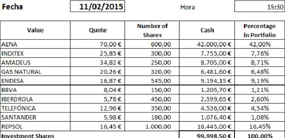
(24) Using the tool solver get the calculation of the optimum weight of actions for the formation of the optimal portfolio, this is the percentage of shares that we will invest in the.. The results obtained are:. Figure 13: “Weight Shares”. Source: Own development.. Therefore our portfolio will be formed finally so:. Figure 14: “Portfolio composition”. Source: Own development.. Aena a percentage of 42% of the portfolio, Inditex with a total of 300 shares and a weight in the portfolio of 7.76%, with a total of 600 shares Amadeus with 250 shares settle 8.71% of our portfolio of investment, Natural Gas 320 actions and 6.48% of the 24.

(25) total amount of the portfolio, with a total of 545 shares Endesa and a total percentage of 9.19% followed by BBVA with 150 shares and 1.21% on the portfolio, Iberdrola with a total of 450 shares and 2.60% portfolio weight, Telefónica with a participation of 350 shares and a weight of 4.54%, composed of 180 actions Santander and 1.08% and finally the company Repsol with a total of 1,000 shares and a total percentage of 16.45% of our portfolio.. 3.3.. CRITICISM OF THE MODEL “ MEDIA-VARIANZA”.. Once the community academic was aware of the revolution caused by the idea exposed by Markowitz began to analyze the detail looking for their points weak. Critical to the model are:. a) Are investors so rational as supposed model?. It can be that investors are rational but their rationality is not adequately captured by the model.. b) Is the variance the proper measure of risk? If not, the model of optimization of combination rendimiento-riesgo still could remain useful by changing the way of measuring the risk. If yields are not distributed exactly as "normal", the variance will not capture all the value of the risk. For investors that this should turn out to be a problem (for others won't) would imply the need to develop other types of strategies.. c) What would happen if the positive relationship of performance and risk were not so?. d) In the years following the development of the model there was a serious technical problem: the cost of calculating an efficient border was very high in dollars (several thousand in the Decade of the 60's of the 20TH century) and in time because the resources of the time were almost in prehistory.. Despite the criticisms of the theory of Markowitz portfolio selection, its contribution has been fundamental. Thanks to it the diversification is has become in a species of religion among the investors.. 25.

(26) 4. HEDGING WITH FUTURES. 4.1.. DAILY PROFITABILITY PORTFOLIO. To start shaping the work and to find the way to more efficient coverage, we will have to make the download of files obtained in the MEFF to perform further calculations.. We need the historical quotes daily for each of the shares of the companies that make up our portfolio, from 11/02/2015 until 19/04/2016, a period covering a little more than one calendar year and that we have a large enough number of variables so that the empirical study is workable, with a total of 302 variables, when we have collected all necessary data will begin to perform the calculations.. Figure 14: “Investment in Shares”. Source: Own development.. By multiplying the price daily for each of the actions that make up our portfolio, we will obtain the cash and the participation offered by that company in our portfolio total. The sum total of these troops comprise investment in securities that we have made to our portfolio, recalling that we had set ourselves a number of investment € 100,000 and the acquisition of the portfolio not could exceed this budget.. We will make exactly the same calculations for all the days of our time horizon, we will have to make it 303 times, process that will make quicker with the Excel tool.. 26.

(27) Figure 15: “Graphic Portfolio Value”. Source: Own development.. Drawing the graph of the value of the portfolio in euros, we can observe that there are periods of earnings and other major losses, since we know that the bag is never constant and you have big oscillations and fluctuations in the stock prices. Most importantly to comment this graphic is the evolution of our portfolio, beginning with an investment of a cash of 99.998,50€ for the day 11/02/2015 and finishing our temporal axis one year after 11/04/2016 with an effective portfolio of 125.556,76€.. 4.2.. CORRELATION COEFFICIENT. He following step that are going to make is find the correlation coefficient between our portfolio and the IBEX 35, to see if there is or not a relationship linear between both and find out if can use it in our experiment.. Calculating this coefficient we want to ensure that the index used for hedging is ideal, and we get so few results as beneficial as possible for our research and find more efficient hedging.. The correlation coefficient of Pearson, intended for quantitative variables (minimum interval scale), is an index that measures the degree of covariation among different variables linearly related. This means that you can have variables strongly related, but not in a linear fashion, in which case not proceed to apply the Pearson correlation. 27.

(28) The advantage that has this coefficient on other tools to measure the correlation, as it can be the covariance, is that the results of the correlation coefficient are limited between - 1 and + 1. This feature allows us to compare different correlations in a way more simple, visual, and standardized.. The value of the correlation index varies in the range [-1,1]: . If r = 1, there is a perfect positive correlation. The index indicates a dependency total between them two variable called relationship direct: when an of them increases, the other also it makes in proportion constant.. . If 0 < r < 1, there is a correlation positive.. . If r = 0, not there is relationship linear. But this does not necessarily imply that the variables are independent: there may be still non-linear relationship between two variables.. . If -1 < r < 0, there is a negative correlation.. . If r = -1, there is a perfect negative correlation. The index indicates a total dependency between two variables called inverse relationship: when one increases, the other decreases in constant ratio.. To know if this index has a high correlation with the portfolio and we can use it in our study we will calculate. it using the Excel tool, by using the command. “=COEF.DE.CORREL(”. . Coefficient of correlation between the portfolio and the IBEX 35:. Calculating the profitability daily of our portfolio and the profitability daily of the counted of IBEX get them two matrices necessary to solve the formula.. With that we get a result from: 0,74263054. This explains our portfolio and the Ibex 35 are positively correlated in a 74%. . Coefficient of correlation between the portfolio and the future of IBEX 35:. Daily profitability of our portfolio and the daily cost of the future of IBEX, we obtain the two matrices to solve the formula.. 28.

(29) With that we get a result from: 0,7261612. This explains our portfolio and the future on Ibex 35 are positively correlated in a 72%. . Correlation coefficient between the IBEX 35 and the future of IBEX 35:. By calculating the daily return on cash of the IBEX 35 and the daily return on the future of IBEX, we obtain the two matrices to solve the formula.. With that we get a result of: 0,98736862. This explains that IBEX 35 contracts and the future on Ibex 35 are highly correlated in a positive way in a 98%.. With these data, we can say the choice of this index for the use of contracts for the future on IBEX 35 in our hedging transaction. With totals above 70%, we can agree that although the coefficient is not perfectly linear, there is a high correlation by both variables and we can obtain results as efficient and reliable as possible.. Then the high correlation between our portfolio and the future on Ibex makes us decide by this type of contract for coverage. To know a little more of the characteristics of these contracts of futures on indices, we consult the website of the MEFF (Spanish official market of financial futures and options), where we can find all the necessary information about this type of contracts.. Conditions on IBEX 35 futures contracts are standardized and described in the MEFF follows:. ACTIVO. Índice IBEX 35.. SUBYACENTE DESCRIPCION DEL INDICE. El IBEX 35 es un índice ponderado por capitalización, compuesto por las 35 compañías más líquidas que cotizan en el Mercado Continuo de las cuatro Bolsas Españolas. 10 euros. Es la cantidad por la que se multiplica el índice. MULTIPLICADOR. IBEX 35 para obtener su valor monetario. Por tanto, cada punto del índice IBEX 35 tiene un valor de 10 euros. 29.

(30) En cada momento, el nominal del contrato se obtiene NOMINAL DEL CONTRATO. multiplicando la cotización del futuro IBEX 35 por el multiplicador. De esta forma, si el futuro IBEX 35 tiene un precio en puntos de 10.000 su correspondiente valor en euros será: 10.000 x 10 = 100.000 euros. En puntos enteros del Índice, con una fluctuación mínima. FORMA DE COTIZACION. adecuada según la cotización del Activo Subyacente y/o las necesidades del mercado, lo que se establecerá por Circular. La fluctuación mínima podrá ser distinta en Operaciones negociadas directamente entre Miembros.. FLUCTUACION. No existe.. MAXIMA Estarán abiertos a negociación, compensación y liquidación:. - Los diez vencimientos más próximos del ciclo trimestral Marzo-Junio-Septiembre-Diciembre. VENCIMIENTOS. - Los dos vencimientos mensuales más próximos que no coincidan con el primer vencimiento del ciclo trimestral. - Los vencimientos del ciclo semestral Junio-Diciembre no incluidos anteriormente hasta completar vencimientos con una vida máxima de cinco años.. FECHA DE. Tercer viernes del mes de vencimiento.. VENCIMIENTO ULTIMO DIA DE. La Fecha de Vencimiento.. NEGOCIACION El precio de liquidación diaria del primer vencimiento se PRECIO DE. obtendrá por la media ponderada por volumen de las. LIQUIDACION DIARIA. transacciones ejecutadas en el libro de órdenes entre las 17:29 y 17:30 con un decimal.. PRECIO DE. Media aritmética del índice IBEX 35 entre las 16:15 y las. LIQUIDACION A. 16:45 de la Fecha de Vencimiento, tomando un valor por. VENCIMIENTO. minuto.. LIQUIDACION DIARIA. Antes del inicio de la sesión del Día Hábil siguiente a la fecha. DE PERDIDAS Y. de transacción, en efectivo, por diferencias entre el precio de. 30.

(31) GANANCIAS. compra o venta y el Precio de Liquidación Diaria. A modo de ejemplo, una compra de 30 Futuros IBEX 35 a 10.000 con un Precio de Liquidación a final de sesión de 10.020 tendrá la siguiente liquidación: (10.020 - 10.000) x 30 x 10 = + 6.000 euros.. LIQUIDACION DE. Primer Día Hábil posterior a la fecha de la transacción.. COMISIONES LIQUIDACION A. Por diferencias con respecto al precio de liquidación a. VENCIMIENTO. vencimiento. Variable en función de la cartera de Opciones y Futuros (ver. GARANTIAS. apartado Cálculo de Garantías). Se suministrarán antes del inicio de la sesión del Día Hábil siguiente a la fecha del cálculo.. HORARIO DE. Desde las 8:30 a.m. hasta las 9:00 a.m.. SUBASTA HORARIO DE. Desde las 9:00 a.m. hasta las 20:00 p.m.. MERCADO Figure 16: “Future conditions”. Fuente: MEFF.. All the information described above, we make special emphasis on the key factors of a futures contract that are: the Nominal amount of the contract, the subject and due date.. Nominal of the contract: "at any time, the nominal value of the contract is obtained by multiplying the price of future IBEX 35 by the multiplier. Thus, if the future IBEX 35 is priced at 10,000 points its corresponding value in euros will be: 10,000 x 10 = 100,000 euros.” Since our investment portfolio has been €100.000 we will have to sell a single contract for the future on Ibex 35 for coverage of our portfolio, if we take more than one futures contract would be about covering our portfolio. Remember that our interest not is get benefit of those markets in future. At this point we will be more restraint and focus only on the coverage of our portfolio to not incur losses.. 31.

(32) Date of expiration: "Third Friday of the expiration month". We will have to take into account the expiration date of each contract for the future, since it has a period of 1 year, at the end of each month we will have to make a roll-over at the end of each contract.. Portfolio / Future IBEX 35 €140.000,00. €130.000,00. €125.556,76. €120.000,00. €110.000,00. €103.590,00 €100.000,00. €99.998,50. €90.000,00. €88.125,00. €80.000,00. Figure 17: “Graphic Comparative Portfolio/Future”. Source: Own development.. The line continues shows the evolution of the value of our portfolio during all the period of coverage. And the dashed line, the price of the future on Ibex 35.. Well looking at the graphics give us realize that both are almost identical and vary and fluctuate in hand, what really draws our attention is the downward trend of the index, which registered its biggest fall since the 2011 7.15 percent, the worst balance since the entry into the financial crisis.. This explains that the contributions of the major Spanish companies have been affected by the Spanish economic uncertainties and geopolitical tensions in the current world scene.. 32.

(33) 4.3.. REALIZATION OF HEDGING .. For make it hedging in the market of counted open our position buying the portfolio of actions and will make the operation counter in the market of future, by what will choose by a position selling of 1 contract of future.. Performing this operation for each date of expiration monthly, and performing a "rollover" to continue the coverage with the following contract after the date of expiration. Until the entire 13 months, which is our investigation period.. For the calculation of the coverage we will need to download the files from the closing price of the Ibex 35 index, both in cash as of the futures contracts, by multiplying the closing price for 10€ you will obtain the nominal value of each contract for the future.. Figure 18: “Nominal future contract”. Source: Own development.. Performing the logarithm napierian of the price of closing of the future and subtracting the price in t-t-1, obtain the profitability daily of the contract's future on IBEX 35. Data that will need to make the hedging. 33.

(34) Figure 19: “Hedging March 2015”. Source: Own development.. The date of commencement of coverage will be 20/02/2015, just when it starts the first contract of futures on IBEX 35. In the column “Spot Market” we will have to put the value of our portfolio at that date, and “Future Market”, put the nominal of the contract's future on Ibex's closing of that same day. Doing the opposite operation in futures markets: If a position of "Buying" shares in our portfolio we have in the cash market, will have to position ourselves in the market's future as a "sale" of 1 single contract of futures on IBEX 35. Closing our position on the date of expiration of the contract of future the 20 / 03 / 2015, just a month after start it.. As we can see we get a result of 4.670,77€ operating in the spot market, a result that is sees diminished by the compensation that suffer to the get losses in the future market, getting losses by - 6.717,00€.. The difference between the results in both markets will be the total result obtained by the coverage, the loss of the – 1.500,06€.. Figure 20: “Hedging January 2016”. Source: Own development.. 34.

(35) As we can observe one of coverages that most attention us for its effectiveness is that of January 2016, which have covered more than the 95% of the portfolio. Where would have incurred in 11.695,43€ of losses in the market of cash had not been carried out coverage, which covers us almost all of this loss. With the benefit the market's future of 11.193,00€ see very reduced the loss of the portfolio to get to a result end of -502,43€.. Figure 21: “Hedging September 2015”. Source: Own development.. Also can highlight the hedging of the contract of September of 2015 by its difference between them prices of cash and future and the excessive benefit retrieved thanks to make the hedging. We went from a loss of- 811,73€ have obtained in a final 4.743,27€ results, thanks to the large profit margin that left us coverage of 5.555€.. As discussed above, obtain benefits with future markets is better than getting lost, yet is not a good indicator for coverage already on our portfolio we cover and do not intend to gain a few extra with this, if not, simply to cover us against the risk of falling profitability of our portfolio. Remember that our goal is to obtain a result of 0€, farther away from this number less effective will be.. Having done all the time horizon of our coverage 13 coverage, we will get these results keeping the hedging until the end and terminating the contract the last day of the date of expiration.. Then spend to perform the same process but with some modification, for to observe how is behaves in this case the hedging and if is more or less effective what which just of calculate.. 35.

(36) But the end of this work is to remove a conclusion clear of what type of coverage has a greater efficiency, by that will make the same process with them 13 coverage, with the difference of that not will keep our position until the end of the maturity, if not that will leave of our position a week before expires the contract, varying so them results obtaining several scenarios to see better the behavior of both coverage and being able to perform a comparison at the end of the project.. Figure 22: “Hedging March 2015 before date expiration”. Source: Own development.. For the second coverage will make the same calculation only will use data from the week before expiration of the contract. We note that this happens earlier, getting a result of 6.859,58€ result what is offset partially by the losses in the futures market with the contract to sell the ibex, which are 3.312,00€. Using the position counter in each one of them markets for the realization right of the coverage. The final result of the hedging obtained is 3.547,58€.. This is a clear example of the double-edged weapon which can be a coverage, when, in the cash market, we could have obtained a profit of almost 7,000 euros, we obtain a result of little more than 3.000, since we have covered more than 50% of the portfolio. And let us remember that when making the opposite position in the futures market we eliminate both the risk of losses and the risk of profit.. 4.4.. HEDGING IN DATE OF EXPIRATION .. Below we show here a table summary of the results obtained in the above explained coverage and which will discuss in depth:. 36.

(37) Figure 23: “Summary Table Hedging in date expiration”. Source: Own development. On the one hand, in the column of “Spot Result” have the result that we have retrieved in the market spot with our portfolio that constitutes a result end of 12.817,67€. In the second column you can see the result we have achieved with our position in the future market, this should compensate possible losses of spot, But what makes the hedging is eliminating the risk of our portfolio, eliminating both the risk negative of possible losses and as the risk positive of possible profits, with a total of 17.271,00€.. The Total Result get it making the difference between the result of the spot market and result in futures markets, this being the final result of our hedging that adds a total amount of 30.088,67€. So that the hedging was perfect, this result should be 0, instead we get revenue to do it, what makes us say that coverage is not perfect and therefore is not fully effective. In the last column of “% Hedged” between the spot market and the future market is calculated as by one hundred it all of it portfolio that managed to cover with our strategy of hedging. Values close to 100% would indicate that our coverage is very effective, to cover almost all of the risk on our portfolio, example we can comment on March 16, earning a 98% coverage, offsetting gains from 9.335,34€ with losses in the future by a total of 9.149,00€ market, leaving the final outcome in 186,34€ and not benefit disproportionately that procured before. It should be remembered that the coverage is a double-edged weapon, eliminating the risk of the portfolio, but both the positive and the negative, the benefits will be undermined by this.. 37.

(38) On the other hand, the coefficient of correlation calculated on the result retrieved in the market of cash with our portfolio of actions and the result of the market's future is of a 88,41%. This means a high correlation between both markets and the effectiveness of the index IBEX 35 used for the hedging.. €15.000,00 €10.000,00 €5.000,00 €€(5.000,00). €(10.000,00) €(15.000,00) Spot Result. Future Result. Figure 24: “Graphic Hedging in date expiration”. Source: Own development.. Making graphics effectively we can determine that almost in all of the coverages the result of spot is partially offset by the result in the future market.. The highest peaks are concerned with profits in one of the two markets, both in cash and in future, and lower peaks represent losses obtained in one of two markets.. As Interestingly we can point out that in some cases the markets do not behave as theoretically explained, for example, let's look at the month of April, where we have achieved gains in both markets and therefore, effectiveness of coverage has been disastrous.. This occurs frequently in this type of coverage, since to the be data real the efficiency of the coverage is much more variable, it will explain later.. 38.

(39) 4.5.. HEDGING A ONE WEEK BEFORE EXPIRATION. In the same way we did the hedging on expiration date, we carry out the same hedging, leaving us one week prior to the position before the expiration date, so to be able to compare the effectiveness of both.. The results obtained in both covers are very similar, being the minimal difference. In the next section we will discuss more in depth the similarities and differences of both hedging.. Figure 25: “Summary Table Hedging a week before date expiration”. Source: Own development.. In the table above in the Spot Result we get the results of our portfolio of stocks in the cash market in which we have achieved a total profit of 9.061,14€. In the next column we have Future Result, where are the results obtained by trading in the futures market with a contract for the future on Ibex 35, obtaining final results of18.703,00€.. In total result we have provided the difference between the result that we get in the spot market and obtained in the future, and this is the end result of our hedging, a total of 27.764,14€. Last column of “% Hedgeg” We get as percent as effective or hiding has been our hedging. Values ends and distant to the 100% us indicate a bad hedging, both positive. 39.

(40) as negative, of example can put it of June of 2015 with a 675%, in which have retrieved 4.283,10€ of benefit, that as have commented previously although obtain some income extra of perform hedging this not is its function.. €20.000,00 €15.000,00 €10.000,00 €5.000,00 €€(5.000,00) €(10.000,00) €(15.000,00) Spot Result. Future Result. Figure 26: “Graphic hedging a week before date expiration”. Source: Own development.. The same happens when we close our position a week before the due date, observing the graph we see the benefits or losses that we obtain in the spot market with our portfolio, compensate them partially with losses or gains in the futures market with our contract for the future on IBEX 35.. As in the hedging above them peaks more high is refer to benefits obtained by the operations in them markets both of counted as of future. On the other hand the grooves correspond to losses obtained with our operation in both markets.. 40.

(41) 4.6.. COMPARISON OF BOTH HEDGINGS. HEDGING RESULT €12.000,00 €10.000,00 €8.000,00 €6.000,00 €4.000,00 €2.000,00 €€(2.000,00) €(4.000,00) €(6.000,00) In expiration date. One week before exp dete. Figure 27: “Graphic Result Hedgings”. Source: Own development.. As we can see the smooth line corresponds to the hedging to date of expiry and the dotted line performed 1 week before due date. Both fluctuate in unison and practically in the same direction.. The coverage in expiration gives ones worst results for the first half of the shaft temporary, obtaining some peaks more high and therefore more away of our hedging perfect, that would be result 0€. Moreover envision that the hedging in which cancel our position a week before expiration provides the worst results in the second half of our axis temporary.. Another interesting comment is that we observe a much more abrupt fluctuations at the beginning of the hedging the first months, fluctuations that are diminishing their size and behaving in a more calmly towards the end of our hedging.. Looking at the chart we see that hedging is not an exact science, I get not always efficient hedging while maintaining the future up to the expiration date, or we obtain greater effectiveness to leave us before the expiry date, the results are very variable and mostly very even in both positions. 41.

(42) ACCUMULATED HEDGING RESULTS €35.000,00 €30.088,67. €30.000,00 €25.000,00. €27.764,14. €20.000,00 €15.000,00 €10.000,00 €5.000,00 €-. €(5.000,00). In expiration date. One week before exp.date. Figure 28: “Graphic Result Accumulated Hedging”. Source: Own development.. If we draw a graph with the cumulative result we see more clearly that both covers reflect earnings way up. With a total of 30.088,67€ of benefits with hedging in expiration (dashed line). By the other side we get with the hedging made before a week of the expiration (line smooth) a total of 27.764,14€ of benefits. The difference of €2.324,53 between two hedges tells us that, although the difference is minimal, keeping the coverage until the date of expiry of the contract you get greater efficiency and therefore a greater result.. At the point designated in February 2016 we get the exact moment where cross the results obtained in the two coverages, this means, the exact spot where both are the same and therefore get the same efficacy.. Fits highlight that in the whole of the horizon temporary of our 13 coverage have acted of a way similar, being them benefits by over an of another almost insignificant as to to take a decision clear of which of both is best.. But if we have to decide for one, we would actually choose hedging outside of the due date, even if it has a positive result is the closest to 0€. 42.

(43) 4.7.. EFFECTIVENESS OF HEDGES. BECAUSE THE COVERAGE NOT IS PERFECT .. We understand by perfect hedging that provides a global null result, i.e. an exact compensation between the results obtained in the position of cash and future. The imperfect hedging can give place to results global positive or negative, or what is it same, situations, in which the operation of hedging goes accompanied of the obtaining of benefits or losses extraordinary, respectively.. Naturally, the coberturistas want to lower completely the risk lurking to its portfolio, i.e., that the results do not deviate from expected. An indicator that lets you know this is the base.. The Basis is: Basis = Spot Price – Future Price. The necessary condition for perfect hedging is that the base is constant.. The reasons why is not met this requirement are as follows: 1º. The use of 2 different products for hedging.. The use of them future on the index IBEX 35 instead of the use of contracts on future of shares belonging to them of the portfolio, is the greater factor of that the hedging made is imperfect.. 2º. So the basis is constant it is necessary company liquide operation on the expiration date. We get rid of the position before the expiration date.. A feature of the market's future is that their date of maturity is a date standard. This condition does not allow that base, i.e. the difference between the future and spot price, is constant. (Recall that the fundamental difference between the future and the contract term is the first market contracts are standardized and the second not).. 43.

(44) 3º. The amount of the nominal value of the futures contract does not match the amount in euro of our portfolio, so we can not cover the total of the money we have invested in our portfolio.. The amount of our portfolio is 100,000€ and the nominal value of each futures contract is the price of the IBEX 35 by a 10€ multiplier, first contract is 107.821,00€.. 4º. The payment of commissions to the intermediary, that coverage is hardly perfect.. 44.

(45) 5. CONCLUSION. With the completion of this work were looking for a clear answer several questions: what is most effective for my hedging, hold it until maturity or cancel the position before this date?, what instruments are more suitable to perform efficient hedging?, which have managed to respond and clarify these doubts.. Begin speaking of the use of them future on the index IBEX 35 as hedging, in the point of the correlation can observe clearly a high correlation with our portfolio and with this type of contracts, more than one 70% of correlation positive, which us guarantees that the hedging get a greater probability of show us results effective.. Once analyzed and compared the coverage we can conclude with that I get more effectively with the hedging made canceling the position a week before due date, with a total result of 27.764,14€ against a total result obtained by hedging maintained until expiration of 30.088,67€.This last is away more than the hedging perfect, that would be a result of 0€, it all of the gain or loss in the market of counted is would be compensated with it all of the gain or loss in the future market. It does so because the main reason products chosen to cover the hedging are different, and so coverage may not be perfect.. Therefore, although the difference is minimal and no large monetary differences between both hedging, we ratify that hedging which comes closest to 0 will be the clear winner of greater efficiency.. This would be in terms of efficiency, purely theoretical, but it is worth mentioning that one bad effectiveness can make us to make money, this is what happens with the hedging kept until maturity, we get some side incomes exceeding the most effective. Although this was not the factor analysis since we focus on the effectiveness of the same, it is consistent to point out this, we can get a few extra additional income, which many companies would like to get.. The possibility of extending the study in the future is a feasible project, because although we have obtained good results with the future on IBEX 35, the possibility of obtaining some best results are high, and can use other instruments to carry out still. 45.

(46) more efficient coverage, as for example the use of stock futures, recreating a hedging with the actions that compose the portfolio.. 46.

(47) 6. BIBLIOGRAPHY. . Jiménez, J. L. (Coord) (2009): Dirección Financiera de la Empresa, 2ª ed.,Ed. Pirámide, 452-456.. . Ferrando, M.; Gómez, A. R.; Lassala, C.; Piñol, J. A.; Reig, A. (2005): Teoría de la Financiación I, Ed. Pirámide.. . Juan Mascareñas (2012).. Mercado de Derivados Financieros: “Futuros y. Opciones”. [2 October 2016] . Juan Mascareñas (2012). Gestión de Carteras I: “Selección de Carteras”. [5 October 2016]. . Juan Mascareñas (2012). Gestión de Carteras II: “Modelo de Valoración de Activos”. [9 October 2016]. . Alizadeh, A. y Nomikos, N. (2004). A Markov regime switching approach for hedging stock indexes. Journal of Futures Markets, 24, 649-674.. . Anderson, R. y Danthine, J. P. (1980). Hedging and joint production: theory andillustrations. Journal of Finance, 35, 487-501.. . CNMV: Comisión Nacional del Mercado de Valores (2006). Guía Informativa: “Qué debe saber de Opciones y Futuros”. [12 September 2016]. . FIRA (2011). Boletín de educación financiera: “Mercados de Futuros y Opciones”. [21 October 2016]. . Salvador Zurita L (2002). Universidad Adolfo Ibáñez. “Cobertura de mínima varianza con futuros”. [18 September 2016]. . Vicent Aragó Manzana (2008). “Teorías sobre cobertura con contratos de futuro”. [15 September 2016] 47.

(48)