Does active management add value? New evidence from a quantile regression approach

Texto completo

(1)Does active management add value? New evidence from a quantile regression approach. ∗. Juan Carlos Matallı́n-Sáez. Amparo Soler-Domı́nguez. Emili Tortosa-Ausina. Universitat Jaume I. Universitat Jaume I. Universitat Jaume I and Ivie. April 2, 2019. Abstract While it has long been recognised that active management is an important issue in the area of mutual fund performance, little consensus has been reached about the value managers’ abilities can add. This study examines funds’ and managers’ characteristics in an attempt to understand their influence on mutual fund efficiency. We explore these issues in a twostage approach, considering partial frontier estimators (order-m, order-α) to assess performance in the first stage, and quantile regression in the second stage to isolate the determinants of efficiency. This combination of methodologies has barely been considered to date in the field of operations research. Our findings are of interest to both academics and practitioners as they shed light on the differences among funds as well as among managers. Our analysis provides some arguments to guide fund selection and points to some managerial features investors might consider taking into account. In addition, some of the differences in performance among funds are rather intricate because both the magnitude of the estimated regression coefficients and their significance varies depending on the quantile of the distribution of fund performance, suggesting that some relevant trends might be concealed by conditional-mean models such as Tobit or OLS.. Keywords: mutual fund, partial frontier, performance, quantile regression JEL Classification: C21, G11, G23 Communications to: Amparo Soler-Domı́nguez, Department of Finance and Accounting, Universitat Jaume I, Campus del Riu Sec, 12071 Castelló de la Plana, Spain. Tel.: +34 964387152, e-mail: [email protected]. ∗. We are grateful to Giacomo Nocera, Nicolas Nalpas, Lucı́a Morales, Manuel J. Rocha Armada, José Luis Sarto and two anonymous referees whose comments have contributed to the improvement of the paper’s overall quality. We would also like to acknowledge the financial support from the Ministerio de Economı́a y Competitividad (ECO201455221-P and ECO2017-85746-P), Universitat Jaume I (UJI-B2017-14 and UJI-B2017-33), and Generalitat Valenciana (PROMETEO/2018/102). The usual disclaimer applies..

(2) 1.. Introduction. Performance evaluation of mutual funds has attracted the interest of researchers and industry participants alike for some decades now. Although in its early stages this literature focused mainly on the design and empirical applications of methodologies to analyse performance (or efficiency), today the factors related to the decision-making process and their consequences for fund efficiency are arousing growing academic attention. In this context, the literature on portfolio evaluation has evolved dramatically since the late eighties. This has partly paralleled the evolution of asset pricing models that consider different methodological approaches, sources of risk and other variables to adjust returns. Since most investments are handled by professional managers, it is important to consider the role they are playing and, if possible, to measure how they can affect performance. Managers have the ultimate power to design a portfolio consistent with their set of objectives and policies. The role of the manager or the team of managers is gaining prominence in fund efficiency analysis. Managers have always enjoyed the limelight because their decisions are directly related to investors’ profits. From a manager’s point of view, the reward scheme is primarily based on economic incentives (fees), although other motivations such as reputation, contracts, or job loss might also underlie their expectations (Brown et al., 1996; Goetzmann et al., 2003; Alexander et al., 2007; Kempf et al., 2009). These and other related priorities may be affected by the decisions taken by each manager or team of managers. Funds have traditionally been managed by individual specialists. However, even in cases where an auxiliary management team is involved, the final decision usually rests with the principal manager. Nowadays, for a significant share of managed funds, teams tend to reach a consensus prior to executing an order. From the point of view of the investor it could seem that the risk of error is more diversified (or more indirect), since the decision does not depend solely on one person. From an academic viewpoint, the way decisions are made has prompted several research initiatives on mutual fund management. Academics are becoming aware of managerial characteristics that can be measured, the influence of which is closely related to the fund’s performance and/or efficiency. It is generally accepted that mutual funds, considered jointly, underperform the market or benchmarks; according to Ferson (2010), performance is typically negative when averaged across funds. However, other approaches, such as those of Ippolito (1989) or Cohen et al. (2005), argue that managers display some skills that enable the funds they manage to beat the market. Our study explores this possibility in an attempt to understand managers’ influence as a source of differences in mutual fund efficiencies. Specifically, in relation to the structure of management, there is no consensus as to whether individual or team management might generate efficiency differentials. 1.

(3) Therefore, as well as estimating the degree of efficiency for each fund, in a second stage of this study we also analyse the determinants of mutual fund performance and/or efficiency, with an explicit focus on the role of managers, in order to identify which factors influence better performance. However, although the study focuses more closely on the role of managers, we split the analysis of determinants into two main sources of variation, or types of information that may influence fund efficiencies, namely: (i) the structure and features of the fund; (ii) some characteristics of the manager or team of managers. We consider frontier techniques to measure efficiency in this study. Specifically, as noted recently by Glawischnig and Sommersguter-Reichmann (2010), interest has been growing in the application of the deterministic data envelopment analysis (DEA) method (without losing sight of more standard methodologies) to measure the performance of financial investments, particularly mutual funds (see also Tarnaud and Leleu, 2018). In this study, we propose going beyond the DEA and related approaches (such as free disposal hull, FDH, its non-convex counterpart) considered so far in the literature to measure the degree of efficiency of each fund since, despite their virtues for measuring mutual fund performance, these methods also have some shortcomings. Specifically, they suffer from a lack of robustness because they are envelopment estimators, and as such they are very sensitive to extremes and/or outliers in the output direction. This ultimately results in poor estimation of the corresponding efficiencies. However, the literature has evolved and has recently proposed two new estimators, namely, the order-m estimator (Cazals et al., 2002) and the order-α estimator (Aragon et al., 2005), both of which are qualitatively robust and bias robust. In this paper we are particularly interested in providing some answers to the puzzling question of whether active fund managers are able to add value. To this end, our second-stage strategy takes into account the fact that the distributions of mutual fund performances can have peculiar shapes, or be heavy-tailed. Under such circumstances, it may be misleading to use regression techniques that focus on the “average effect for the average fund”. Instead, we use a quantile regression approach (Koenker, 2001), which allows us to examine the relationship between the set of managers’ characteristics we consider (along with other likely determinants) at a range of points in the conditional mutual fund performance distribution. This approach is more informative than an OLS regression, for instance, since it might be the case that managerial abilities are more relevant for certain funds—for instance, the highest performing ones—than for the average fund. In addition, whilst the optimal properties of standard regression estimators are not robust to modest departures from normality, quantile regression results are characteristically robust to outliers and heavy-tailed distributions (Coad and Rao, 2008). From an Operations Research (OR) point of view, this is particularly important given that. 2.

(4) performing a second-stage regression can be problematic when the first stage yields efficiency scores obtained via either DEA or FDH (and, to a lesser extent, order-m and order-α). This point has been convincingly made by Léopold Simar and Paul W. Wilson (Simar and Wilson, 2007, 2011), and has had a remarkable impact on the OR literature, resulting in the publication of several contributions on the topic including Banker and Natarajan (2008), Hoff (2007), McDonald (2009), among others. However, the combination of linear programming (OR) techniques to measure efficiency in the first stage, with quantile regression to evaluate the determinants of efficiency in the second stage has barely been contemplated in either the OR or mutual fund performance literatures. When the specific aim is to analyse how different managers’ characteristics might influence funds’ performance combining the two approaches (i.e., DEA/FDH and the like in the first stage, quantile regression in the second stage) the number of studies is virtually zero. Thus, the contribution of this paper is three-fold. First, we explore fund managers’ characteristics and their potential effects on portfolio efficiency. For this purpose, several features of the manager are analysed, focusing particularly on the rise of team-managed funds in the US mutual fund industry—without discriminating other variables that have also gained importance in recent times. We detect that teams of managers are positively associated with fund efficiency. This is a topic that enriches the literature dealing with active management and mutual fund performance, on which contributions based on OR techniques are scarce. Second, building on Abdelsalam et al. (2014), and following recent proposals in the field (Chen, 2019), we propose using a two-stage method which consists of evaluating mutual fund performance via partial frontier estimators in the first stage, in combination with quantile regression in the second stage. In the specific area of manager characteristics and their impact on fund performance, which is thriving (see, for instance Bessler et al., 2018; Ma et al., 2019; Moreno et al., 2018), this approach has not been previously considered. In addition, and from a more methodological point of view, it contributes to the debate in an area in which the issue of the role of environmental variables has not been fully addressed, as shown by Bădin et al. (2014), among others.1 Our results actually show that because the effect of managers’ characteristics (in combination with other fund characteristics) is not constant across the distribution of efficiency scores, it is easy to miss the global impact of covariates, particularly when inspecting the upper and lower tails (best and the worst funds). Finally, our methods are applied to a large updated sample of US mutual funds, classified into several different categories. This is not a contribution per se, but makes the study more appealing to a broader audience. 1. Actually, in some fields such as the determinants of local government performance, some surveys have specifically revised the literature on its determinants (see, for instance Aiello and Bonanno, 2019; Narbón-Perpiñá and De Witte, 2018). More recently, and for the interested reader, Daraio et al. (2019) have reviewed all empirical surveys that, in the field of efficiency and productivity analysis using frontier techniques, are available so far.. 3.

(5) The remainder of this paper is organised as follows. Section 2 presents the methods selected to measure performance and to analyse its determinants. Section 3 describes the data, the fund attributes and the set of determinants. Results are reported and discussed in Section 4. Finally, Section 5 presents some concluding remarks.. 2.. Methodology. 2.1.. Order-m and order-α estimators. As Simar and Wilson (2008) point out, Farrell (1957) first attempted to empirically estimate efficiency scores for a set of observed production units—in our case, mutual funds (Simar and Wilson, 2008, p.421). This first requires us to define the set of attainable combinations of inputs (x) and outputs (y), i.e., the production set, Ψ, which is: Ψ = {(x, y) ∈ Rp+q + |(x, y) are attainable}. (1). where x ∈ Rp+ is the vector of inputs and y ∈ Rq+ is the vector of outputs. For all possible output. values we can define the section of possible values of x as. X(y) = {x ∈ Rp+ |(x, y) ∈ Ψ}. (2). In this particular setting the Farrell (1957) measure of input-oriented efficiency of a given mutual fund with input-output mix (x, y) is defined as e y) = inf{θ : (θx, y) ∈ Ψ} = min{θ : θx ∈ X(y)}, θ(x,. (3). where θ(x, y) is the proportionate reduction of inputs required for a mutual fund with the inputoutput mix (x, y) to become efficient, i.e., to achieve the value of 1, since the efficient frontier e y) = 1. corresponds to those funds whose θ(x,. In the case of output efficiency scores, the production set Ψ is characterized by the output. feasibility sets defined for all x ∈ Rp+ . In this case, for all possible input values we define the set of possible values of y as. Y (x) = {y ∈ Rq+ |(x, y) ∈ Ψ}. (4). In this output-oriented setting the Farrell (1957) measure of output-oriented efficiency of a. 4.

(6) given mutual fund (x, y) is defined as e y) = sup{θ : (x, θy) ∈ Ψ} = max{θ : θy ∈ Y (x)}, θ(x,. (5). According to either DEA or FDH, the efficiency measure is obtained by comparing with the full frontier of all observations, defining the maximum output that is technically feasible with a given level of inputs. Alternatively, according to the order-m estimators, what is actually used as a benchmark is the expected maximum output achieved by any m funds chosen randomly from the population, which employs at most input level x. Therefore, for any y, the expected maximum level is defined as: e y∂ = θy.. (6). When we choose a high value for m (m → ∞), the order-m estimator gives the same benchmark. as FDH, yielding the same results. Therefore, the most interesting cases are those for which we. define a finite value for m. In these cases the order-m does not envelop all the data, as it is more robust to data outliers. Note that the order-m efficiency scores are not bounded by 1 as in the case of DEA or FDH. In these cases, values equal to unity correspond to efficient funds, whereas values higher than unity correspond to inefficient funds. Order-m can yield values for θ lower than one, indicating that the fund operating at the level (x, y) is more efficient than the average of m peers randomly drawn from the population of units using fewer inputs than x. Formally, the proposed algorithm (Cazals et al., 2002) to compute the order-m estimator comprises the following steps, for n funds, i = 1, . . . , n: 1. For a given level of x0 , draw a random sample of size m with replacement among those xi , such that xi ≤ x0 . 2. Obtain the efficiency measures, θei . 3. Repeat steps 1 and 2 B times and obtain B efficiency coefficients θeib (b = 1, 2, . . . , B). The quality of the approximation can be tuned by increasing B, but in most applications B = 200 seems to be a reasonable choice (and this coincides with ours). 4. Compute the empirical mean of B samples as: θ̄im. B 1 X eb = θi B b=1. 5. (7).

(7) A similar estimator to order-m, and that shares some of its underpinnings is the order-α quantile-type frontier. The idea of order-α is the opposite of order-m: whereas the m parameter of order-M almquist serves as a trimming parameter for tuning the percentage of points that lie above the frontier, in the case of order-α the frontier is determined by first fixing the probability (1 − α) of observing points above the order-α frontier. Therefore, with order-α we reverse the. causation and choose the proportion of the data lying directly above the frontier.. Order-α partial frontiers were originally proposed by Aragon et al. (2005) in the univariate case and were extended to the multivariate case by Daouia and Simar (2007). Similarly to the order-m estimators, order-α estimators also have better properties than the usual nonparametric frontier √ estimators (either DEA or FDH). They are n-consistent estimators of the full frontier, since the order of the frontier is allowed to grow with sample size. They are asymptotically unbiased and normally distributed with a known expression for the variance (see Aragon et al., 2005). It has also been shown (see Daouia and Simar, 2007) that order-α frontiers are more robust to extremes than order-m frontiers (see Daraio and Simar, 2007, p.74). Yet the main virtue of order-α estimators is the same as that of order-m, i.e. the fact that in finite samples, order-α estimators do not envelop all the data, and they are therefore more robust to outliers than FDH or DEA. These outliers which, in the particular output-oriented case we are dealing with have an efficiency score of 1, are considered as super-efficient with respect to the order-α frontier level. In addition, analogously to order-m partial frontiers, where a mutual fund operating at (x, y) is benchmarked against the expected maximum output (recall we are dealing with the outputoriented case) among m peers drawn randomly from the population of funds with output levels of at least y, in the case of order-α quantile frontiers the benchmark is the output level not exceeded by (1 − α) × 100% of funds among the population of funds providing input levels of at least x.. Following Simar and Wilson (2008), for α ∈ (0, 1], the α-quantile output efficiency score for. the mutual fund operating at (x, y) ∈ Ψ can be defined as. θα (x, y) = sup{θ|Fy|x (θy|x) > 1 − α}. (8). We have that θα (x, y) converges to the FDH estimator θ(x, y) when α → 1. As indicated in. Daraio and Simar (2007), in cases where θα (x, y) = 1, the fund is “efficient” at the level α × 100%,. since it is dominated by mutual funds providing less input than x with probability 1 − α. In those cases where θα (x, y) > 1 the unit (x, y) has to increase its output to the level θα (y, y)x to achieve the output efficient frontier of level α × 100%. We can also apply the plug-in principle to. obtain an intuitive nonparametric estimator of θα (x, y) = 1 by replacing Fy|x (·|·) with its empirical 6.

(8) counterpart to obtain: θbα,n (x, y) = sup{θ|Fby|x,n (θy|x) > 1 − α} 2.2.. (9). Analyzing the determinants of mutual fund performance using regression quantiles. Typical linear models such as ordinary least squares (OLS) or logistic regression models (e.g. Tobit) have for years been the workhorse of applied economics and finance researchers. They provide the analyst with information that, albeit extremely valuable, is confined to the analysis of average impacts of the covariates on the variable of interest—in our case, mutual fund performance. Unfortunately, this implies missing relevant information, since the impact over the entire conditional distribution of efficiencies could vary depending on different parts of the distribution such as the upper and lower tails or, more generally, on each particular quantile (Coad and Hölzl, 2009). The analysis of the differential impact on each quantile is actually possible using quantile regression (see, for instance Buchinsky, 1998; Taylor and Bunn, 1999), the main advantage of which is its capability to estimate the conditional quantiles of a response variable distribution— which in our case would be the performance of mutual funds—in a linear model providing a fuller view of the likely causal relationships between the variables considered in the analysis. Quantile regression has additional advantages that are particularly suited to the application we are dealing with, since social phenomena are usually plagued with non-standard conditions such as non-normality or heteroskedasticity. These conditions make it difficult to meet the assumptions on which OLS models are based. For instance, managerial finance data such as the dispersion of the annual compensation of chief executive officers is usually expected to increase with firm size, suggesting the existence of heteroskedasticity. Taking into account the advantageous features of quantile regression, applications have flourished over the last few years, a compendium of which is provided by Fitzenberger et al. (2002). Therefore, in the setting we deal with here, quantile regression allows us to consider the entire distribution of mutual fund performances when analysing how the different covariates impact on performance, providing us with a more complete view of the relationship among variables. Accordingly, we can examine whether the sign and significance of the determinants is the same for low-performance mutual funds (i.e. those corresponding to the lower quantiles) as for highperformance funds (i.e. those corresponding to the highest quantiles). It is then possible to more precisely disentangle the factors which cause mutual fund performance to differ. These arguments imply that we consider both high- and low-performance funds to be of interest per se, as well as those corresponding to other quantiles of the conditional distribution. 7.

(9) In the field of finance and mutual fund evaluation, the relatively modest number of studies using quantile regression methods has been growing in the last few years. For instance, Bassett Jr and Chen (2001) use regression quantiles to extract additional information from the time series of returns by identifying the way style affects returns at places other than the average. Meligkotsidou et al. (2009) introduce the idea of modelling the conditional quantiles of hedge fund returns using a set of risk factors, whereas Luo and Li (2008) investigate whether and how futures market sentiment and stock market returns heterogeneously affect the trading activities of institutional investors in the Taiwan spot market. The aims of our paper are closer to those of Füss et al. (2009), who analyse the impact of experience and size of hedge funds on performance, or Chen and Huang (2011), who study the relation between mutual fund performance and Morningstar fiduciary grades, in both cases using quantile regression. However, none of these contributions has considered partial frontier methods to evaluate performance in the first stage of the analysis, nor have they taken an explicit approach to analyse how the covariates that more closely reflect managers’ characteristics influence mutual fund performance. It can, however, be troublesome to consider a two-stage method in which efficiencies are obtained using, for instance, DEA or FDH in the first stage, and then analysing determinants in the second stage. Simar and Wilson (2007) proposed a bootstrap method that overcame many of the difficulties found in the previous literature—which were mostly related to the combination of nonparametric methods such as DEA or FDH in the first stage with parametric methods such as OLS or Tobit regressions in the second stage.2 Other approaches to deal with this issue include, for instance, Banker and Natarajan (2008). In the particular case of mutual fund performance evaluation, Daraio and Simar (2006) have proposed alternative nonparametric methods to overcome the problems derived from estimating regressions where the dependent variable is obtained by solving linear programming problems. In this scenario, an additional advantage of using quantile regression in the context of evaluating the determinants of mutual fund performance is that the standard least-squares assumption of normally distributed errors does not hold for our data because the location patterns follow a fattailed distribution (Coad and Hölzl, 2009). However, although standard regression estimators are not robust to departures from normality, the quantile regression estimator is characteristically robust to outliers on the dependent variable (Buchinsky, 1998). Furthermore, quantile regression also relaxes the restrictive assumption that the error terms are identically distributed at all points of the conditional distribution. Avoiding this assumption makes it easier to analyse discrepancies in the relationship between the endogenous and exogenous variables at different points of the 2. For instance, the efficiency scores obtained using linear programming techniques are dependent by construction.. 8.

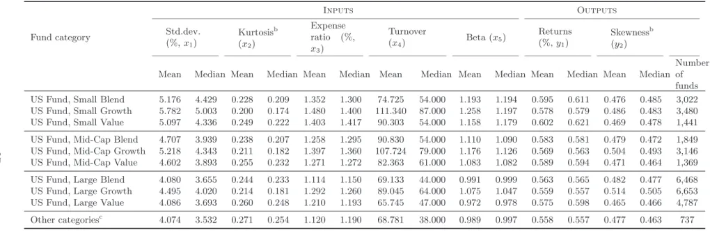
(10) conditional distribution of the dependent variable, i.e. mutual fund efficiencies. The regression quantiles specify the τ th quantile of the conditional distribution of yi , where yi is the variable containing the performance of mutual funds which, in our case, are either θ̄im or θbα,n , given x as a linear function of the covariates. Estimation is performed by minimizing the. following equation:. X. Min. β∈Rk. i∈{i:yi ≥x′ β}. τ |yi − x′ β| +. X. (1 − τ )|yi − x′ β|. (10). i∈{i:yi <x′ β}. where k is the number of explanatory variables, τ represents the vector containing each quantile, and the vector of coefficients to be estimated, β, differs depending on the particular quantile.. 3.. Data and sample. 3.1.. Data sources. We obtained equity fund data from Morningstar. Our data correspond to US mutual funds, and the sample period runs from January 1st , 2000, to December 31st , 2016. The sample comprises the universe of open-end funds domiciled and available in the US, and comprising different categories of funds, as shown in Table 1. Although the nine main categories of funds correspond to the combinations of large, mid-cap and small with value, blend and growth, there are also some other categories which we also included in the sample. However, these other categories contain a much lower number of funds (737 fund-year pairs) compared to the 32,222 corresponding to the nine main categories. Therefore, a total of 32,959 fund-year pairs are classified in all categories, and we consider monthly average returns for the aforementioned period (i.e., the number corresponds to the sum of the available funds for each of the 17 sample years, and the number of funds varies depending on each year due to unavailable information or fund creation/disappearance). For each mutual fund, Morningstar provides historical information on some fund characteristics and managerial attributes, as well as the variables that we label as inputs or outputs. Unfortunately, the sample is somewhat smaller than what a priori it could be due to unavailable information for several inputs and outputs for some years. The Morningstar dataset provides information on all mutual funds operating during the period considered. Thus we consider both funds that disappeared during the period and new funds incorporated and, consequently, the data used is free of survivorship bias. 3.2.. Input and output selection. 9.

(11) To apply our methodological approach we define some variables as inputs and outputs. The main output we consider is the daily mean return over the sample period (y1 ), assuming reinvestment of all income and capital gain distributions. The other output (skewness, measuring the asymmetry of the distribution, y2 ) was also computed from the monthly average return distribution. The inputs are the risk of the fund, measured by the standard deviation of the monthly average returns (x1 ), and kurtosis (x2 ),3 also computed from the monthly average returns. In some of the proposed models the degree of active management and costs of the fund are also considered as inputs. Two variables are considered to include them, namely, the expense ratio, representing the percentage paid as management fees including managers’ compensation and operating expenses (x3 ), and the annualized turnover ratio, as a measure of trading activity or the manager’s propensity to trade (x4 ). We also consider the beta as an input, x5 , since it measures the systematic risk, also known as “undiversifiable risk” or “market risk”. Finally, we consider size as a possible source of economies of scale in mutual fund management. We measured size as the average of the amount of managed assets over the sample period. The descriptive statistics for inputs and outputs are presented in Table 1, which also displays the different fund classes considered. Part of the information in this table deserves additional explanations. On average (as well as for the median), the beta for “growth” funds is higher than that for either “blend” or “value” funds, since they invest in stocks with higher levels of systematic risk. The beta is reported by Morningstar, which computes mutual funds’ beta by adjusting the market index depending on the fund’s category. Table 1 also shows that, in the case of “growth” funds, the turnover (x4 ) for the first quartile is, for both the mean and the median, much higher than that corresponding to the other two categories (either “blend” or “value”), which might be indicative of active management. 3.3.. Determinants of mutual fund performance. In order to match our study more closely to the literature on the determinants of mutual fund performance, we define a set of fund-related variables, in addition to considering the aforementioned fund classification—small/mid-cap/large, blend/growth/value. Specifically, we consider two sets of likely determinants of fund performance, some of which are fund characteristics, whereas others are managers’ attributes. The fund characteristics considered are: (i) fund size (in logs), deemed as an indicator of economies of scale; and (ii) age of the fund (in years), assumed to be a reasonable proxy for the competitiveness of the fund. Characteristics of managers or teams of managers 3. In the case of non-normal distributions, Glawischnig and Sommersguter-Reichmann (2010) consider taking noncentral measures by using information about skewness and kurtosis. See also Briec et al. (2007) and Brandouy et al. (2013). We dealt with the negative values found both for both skewness and kurtosis by rescaling both variables.. 10.

(12) considered are: (i) managerial ownership, a dummy variable taking a value of 1 in the case of manager ownership, 0 otherwise; (ii) manager structure, also a dummy variable taking the value of 1 for multiple managers and 0 in the case of a single manager; (iii) number of funds under the same management (i.e., funds managed per manager or team of managers); (iv) tenure of active management, related to managers’ experience which should be an indicator of their investing abilities; and (v) number of funds under the same management (i.e., funds managed per manager or team of managers). 3.3.1.. Fund characteristics. According to Chen et al. (2004), the expected impact of F S (fund size) is that small funds outperform large funds. Ferreira et al. (2013) also find that small US mutual funds perform better than large funds, but this negative size effect is not consistent when non-US funds are considered. However, other scholars such as Carhart (1997) suggest that a positive relationship between fund size and performance may arise from the benefits of economies of scale. The literature assessing the impact of size on performance is therefore not conclusive, and some of these disparate results are reviewed in Bertin and Prather (2009). Our methodologies might fit this context particularly well, since an inconclusive link could be related to varying coefficients for the different quantiles of the conditional distribution of performance. Regarding the other covariate related intrinsic to the fund, Hu and Chang (2008) found that the expected impact of fund age (F A) is that performance worsens with the age of the fund. However, Chen et al. (2004) and Ferreira et al. (2013), among others, find no evidence of a relation between fund age and performance. Again, the evidence is mixed. 3.3.2.. Managers’ characteristics. We assess whether managerial ownership is related to positive past performance. In this regard, Khorana et al. (2007a) find a positive relation between fund manager ownership and performance, observing in particular a link between positive managerial ownership and future performance. They reinforce this evidence considering both the incentives to generate higher performance and also the superior level of information the managers participating in the funds may have. In the same vein, Evans (2008) argues that funds with higher managerial ownership exhibit better performance. In addition, Fu and Wedge (2011) investigate the impact of the investment behaviour—measuring the disposition effect as an anomaly, according to which investors tend to sell winning assets while keeping losing value assets—together with manager ownership and portfolio performance. These authors partly justify the superior performance achieved by the funds that participated 11.

(13) with higher managerial ownership in combination with the absence of the disposition effect. In contrast, Kumlin and Puttonen (2009) report conflicting evidence showing no relation between performance and manager ownership. More recently, Hornstein and Hounsell (2016) find that the positive relation between manager ownership and performance is consistent for solo management, but diluted for team-managed funds. The role of multiple (team) or single managers (M M ) varies, according to studies by Chen et al. (2004), or Bär et al. (2011); team performance has a negative impact compared with single managers’ performance. In contrast, Han et al. (2017) find a positive impact of team management on mutual fund performance. Mid-way between these conflicting views, Prather and Middleton (2002) find no differences in the performance of funds handled by a single manager or by a team of managers. The literature has also considered whether managers’ tenure (T EN ), namely, their years of experience, might also have an impact on fund performance. Malhotra et al. (2007) find no empirical evidence to support this effect. In contrast, Golec (1996) claim a positive relation between tenure and performance. In the same vein, Khorana et al.’s (2007b) results indicate that the best performance is related to longer managerial tenure, similarly to Agarwal et al. (2009), who conclude that experienced managers outperform their inexperienced counterparts. Although the studies supporting the positive link dominate, there are differing views such as those of Boyson (2010), who found that the link is actually negative—performance deteriorates with managerial experience. The effect of the number of mutual funds under the same management (M F ) is examined by Prather et al. (2004), among others, who find that performance worsens when managers handle more than two funds, as a result of reduced effectiveness due to the dispersion of effort, time and consciousness. This result is supported by Hu and Chang (2008), whose findings indicate that a fund’s performance falls when the number of managed funds increases. However, other authors such as Huij and Derwall (2011) conclude that the more concentrated the portfolios, the better the performance, due to some pernicious effects derived from diversification that contribute to eroding performance. Also related to managers’ characteristics, it is interesting to consider other features such as subadvising. As Moreno et al. (2018) have recently pointed out, mutual funds’ managers outsource portfolio management in pursuit of several benefits such as access to talent that is not available inhouse. This allows them to expand their mutual fund family to include new investment styles and, ultimately, increase the volume of assets under management. Outsourcing can therefore improve the efficiency of the portfolios offered, and firms’ managers can gain market share in the mutual. 12.

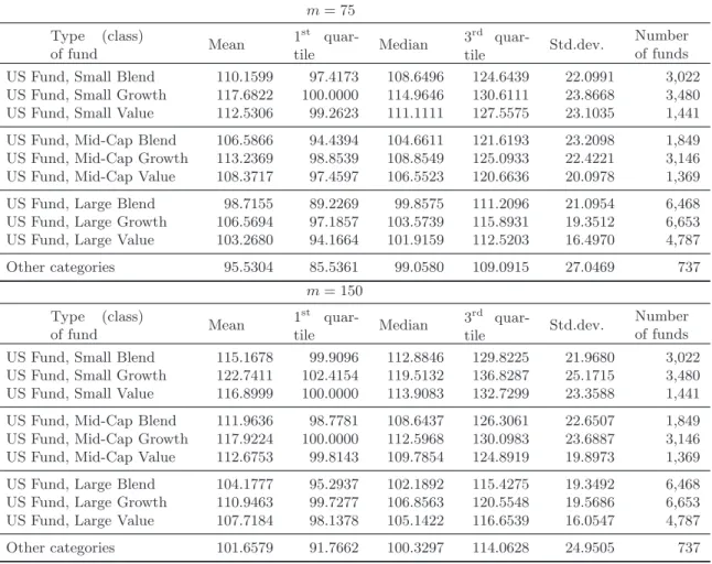
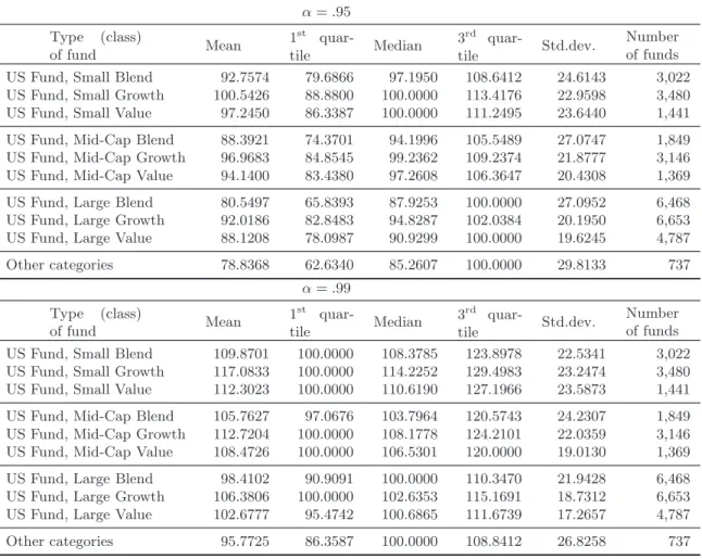
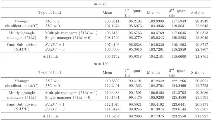
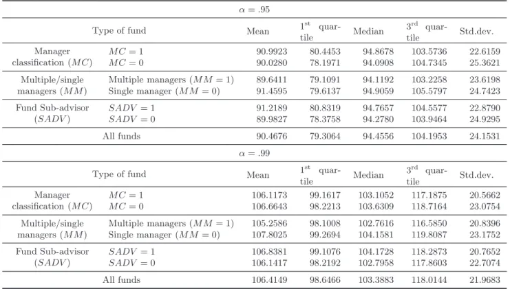
(14) fund industry. The literature is not unanimous on this respect, however, since empirical evidence from Chen et al. (2013) shows that outsourced funds underperform those internally managed. In sum, these are some of the variables that the most relevant literature has considered to analyse how managerial and other related characteristics affect fund performance. However, although much of the reviewed literature has identified strong links between the variables under analysis, in some cases the findings are contradictory. We consider that the methodologies used in this paper, both in the first and second stage of the analysis, can partly explain some of these conflicting views on how the different covariates might impact on fund performance. ——————–. 4.. Results. 4.1.. Expected order-m and order-α efficiency estimates. Tables 2, 3, 4 and 5 report summary statistics (mean, 1st quartile, median, 3rd quartile and standard deviation) for mutual fund efficiencies obtained using order-m and order-α. In both cases results are reported for different choices of the tuning parameters. Specifically, we report results for m = 75 and m = 150, in the case of order-m, and for α = 0.95 and α = 0.99, in the case of order-α. Recall that, for both order-m and order-α, the higher the values of the tuning parameters, the higher the similarities with the results obtained for FDH. The joint evaluation, for all 32,959 fund-year pairs (whose efficiency is measured yearly), is reported in the last row of each panel in Tables 4 and 5. Results are also reported for different classifications of mutual funds. Specifically, we provide results using the manager classification (managerial ownership, M C), multiple vs. single manager classification (M M ), and sub-advising (SADV ). The results according to fund classification are reported in Table 2 (order-m) and Table 3 (order-α), whose upper and lower panels correspond to different values of the trimming parameters (m and α, respectively). As for the interpretation of efficiencies, since we are maximising in the sense Farrell describes, the higher the value of the score, the lower the efficiency level. Therefore, efficiency scores closer to unity indicate that the fund is actually more efficient. A cursory look at the summary statistics reveals that performance varies remarkably across categories of funds (small vs. mid-cap vs. large funds, blend vs. growth vs. value funds, funds with managerial ownership vs. non-managerial ownership, funds managed by single managers vs. funds managed by multiple managers, or the practice of sub-advising), across efficiency measures (order-m vs. order-α), as well as different trimming parameters (m, α). Some stylized facts, however, are robust to these sources of variation. For instance, the funds in the “blend” category. 13.

(15) are more efficient (lower efficiency values), on average, than either “growth” or “value” funds. This result holds regardless of the summary statistic considered—not only the mean but also the 25th , 50th (the median) and 75th quantile. This robustness is also present for funds managed by a single manager, whose efficiency is consistently worse than that of funds managed by multiple managers, regardless of the summary statistic, efficiency measure or trimming parameter chosen (see Tables 4 and 5). However, when comparing funds with managerial ownership with those without managerial ownership (M C), patterns are not entirely robust across any of the dimensions considered. Under such circumstances, one could a priori be inclined to conclude that the differences in performance between these two types of funds are probably not significant. This conclusion calls for a specific test, however. We examine this issue in greater detail in the next few paragraphs. Although it is helpful to use several summary statistics as well as the mean when describing the distributions of efficiency scores, it is even more informative to consider the graphical representation of the entire distributions of efficiencies—obtained either using order-m or order-α. There are several methods to do so, including univariate density functions estimated via kernel smoothing, box plots, or their combination, namely, violin plots. In our view, this convenient combination of densities and box plots makes violin plots a reasonable choice. In this case, the density trace is plotted symmetrically to the left and right of the (vertical) box plot (i.e. there is no difference in the density traces apart from the direction in which they extend). By adding these two densities and the box plot we can compare distributions more easily (our purpose) than using density traces only. Figure 1 represents the violin plots for mutual fund efficiencies. It contains three subfigures corresponding not only to order-m and order-α, but also to the non-robust DEA and FDH methodologies, in order to see more clearly how results vary depending on the methods used to measure performance. Thus, Figure 1a provides violin plots for efficiencies obtained using DEA and FDH. Since we are maximising in the sense Farrell describes, the minimum value is one. Efficiencies above this threshold indicate that the analysed fund could increase its output using the same amount of inputs as those funds on the efficient frontier. As expected, dropping the convexity assumption naturally leads to a much higher number of efficient funds, a result that we can observe in the violin plot corresponding to FDH. The violin plots for order-m are not entirely coincidental. As shown in Figure 1b, results are quite robust to the specification of the trimming parameter (m)—in this case, we considered an additional parameter (m = 100) to see more clearly how results evolve depending on its value. Recall that this parameter allows adjustment of the number of outliers. However, because we. 14.

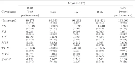
(16) allow for the existence of outliers, we have a substantial amount of probability mass below unity, which causes the shape of the violins to differ markedly from those obtained for DEA and FDH. In fact, we have proper violins for order-m. Finally, Figure 1c displays the violin plots for efficiencies obtained using order-α. In this case we corroborate the magnitude of the impact of modifying the α parameter, which sets the percentage of outliers, as in the order-m case; we also considered an additional parameter (α = .90) to see more clearly how results evolve depending on the trimming parameter. We can also corroborate that order-α results come close to those for FDH when a sufficiently high α parameter is set, as shown by the third violin plot (α = .99). The plots in Figure 1 therefore provide us with a graphical illustration of some features corresponding to each of the techniques considered to measure mutual fund efficiency. Whereas Figure 1a clearly indicates that DEA and FDH do not allow for outliers, Figure 1b and Figure 1c plainly show that the same does not hold for either order-m or order-α. However, in the case of order-α the impact of the trimming parameter can be very strong, as shown by the violin plots corresponding to α = .90 and α = .95, for which the number of outliers (efficiencies below unity) is quite substantial. 4.2.. The determinants of mutual fund performance: fund and managers’ characteristics. Results on the determinants of mutual fund performance, considering the methods to measure performance, are provided in Tables 6 (order-m, m = 75), 7 (order-m, m = 150) and 8 (order-α, α = 0.99). We select a high value of α because it provides results close to those yielded by FDH. Reporting results for other values of the trimming parameter and for other efficiency measurement methods lends additional robustness to the analysis. These tables provide coefficients and standard errors for selected quantiles (τ. =. {.10, .25, .50, .75, .90}). Note that the quantile τ = .50 refers to the median of the conditional. distribution. Whilst OLS regressions report estimates based on the mean, quantile regression based on τ = .50 provides an analogous result for a different moment of the distribution—i.e. the median. Therefore, this median-regression model can be used to achieve the same goal as conditional mean-regression modeling, namely, to represent the relationship between the central location of the response and a set of covariates. However, as Hao and Naiman (2007) indicate, when the distribution is highly skewed, which is the case of efficiency scores (many efficiency scores are located in the vicinity of one), the mean can be difficult to interpret, whereas the median remains highly informative (Hao and Naiman, 2007, p.3). The results in Tables 6, 7 and 8 go further 15.

(17) in this respect, reporting results not only for the median (τ = .5) but also for other quantiles, and are therefore much more informative. In each of these tables (6–8) we provide quantile regression results for all selected covariates (F S, F A, M C, M F , M M , T EN , M F S and SADV ). For each table, the dependent variable is the efficiency of each fund yielded by order-m (with m = 75 and m = 150) and order-α (α = .99). Recall that, as indicated above, since we are maximising in the sense Farrell describes, the higher the value of the score, the lower the efficiency level (efficiencies closer to unity indicate higher efficiency). 4.2.1.. Fund characteristics. The results reported in these three tables clearly show the relevance of this type of analysis because some conclusions could not be reached using other regression techniques such as OLS, or censored regression. For instance, as shown in Table 6, taking into account the values obtained for the first of the funds characteristics’ covariates, namely, fund size (F S), the impact on performance is positive and significant (1%) throughout—recall that we are maximising in the sense Farrell describes, so higher values indicate worse performance, therefore negative coefficients should be interpreted inversely. This result is maintained across quantiles—i.e., regardless of the tau parameter considered—adding additional robustness to the finding. Robustness is also preserved, both in terms of sign and significance of the coefficient, not only when setting other trimming parameters for order-m (m = 150, see Table 7), but also when considering order-α (see Table 8). These strong results do not entirely coincide with previous literature such as Choi and Murthi (2001), who found no links between size and performance and, in general, with our conclusion in section 3.3 that the evidence is inconclusive. Our results therefore suggest that economies of scale might emerge when large fund performance is compared with that obtained for small funds—which might be more inefficient than their larger counterparts due to the associated costs. If conclusions had been based on a conditional-mean model (such as OLS), the information obtained would have been constrained to the average effect. In our case, the conditional-median effect (revealed by τ = .50) would indicate that the median effect is also positive and significant and, in addition, we obtained information for the rest of the quantiles. As for the other variable related to the funds’ characteristics, fund age (F A), its effect on performance is mostly negative (positive coefficient) and significant. In addition, the magnitude of the estimated coefficient is relatively stable—although it is larger for the lowest quantiles (τ = .10) in the case of order-m with m = 75 (Table 6) and order-α (Table 8). This result is very robust, not only for the different quantiles but also for the different measurement methods (order-m and 16.

(18) order-α) and even for the different trimming parameters considered (m = 75 and m = 150). This inverse relation between age and performance is also found in Hu and Chang (2008), implying that performance decreases with the age of the fund or, older funds do not necessarily perform better than newer ones. 4.2.2.. Manager characteristics. We also provide results for the variables related to ownership. Managerial ownership (M C), which can be either positive (M C = 1) or zero (M C = 0), has a generally negative impact (positive coefficient), whose magnitude is large and significant throughout—regardless of the quantile τ or trimming parameter (m) considered (see Tables 6 and 7). Results are robust when extending the analysis to order-α (Table 8). We only find some differences when focusing on the magnitude of the estimated coefficients, which are generally larger for order-m. However, the trend of higher magnitude coefficients for the lowest quantiles is shared both for order-m (Tables 6 and 7) and order-α (Table 8). This result is not entirely in line with the empirical evidence to date. Taking into account the literature revised on page 12, only a few authors such as Kumlin and Puttonen (2009) find this negative association between managerial ownership and performance. However, none of the reviewed contributions considers regression quantiles and, therefore, cannot find that the effect is particularly strong for the best performing funds (higher coefficients). These relatively conflicting views imply that more research is needed, using different methods—if possible. The multiple manager (team) or single manager variable (M M ) is a dichotomous variable taking a value of 1 (in the case of a team of managers) or 0 (in the case of a single manager). Similarly to the manager classification variable (M C) the pattern is mostly negative (positive coefficients) and significant for the vast majority of the quantiles. The only exception is for τ = .90 for order-munder m = 75, although the coefficient is not significant at the usual levels (see Table 6). Therefore, given the demonstrated robustness of the results for the different methodologies, trimming parameters (α, m) and quantiles (τ ), we may conclude there is a strong link between performance and whether managers operate in a team or individually which, in this case, does not favour teams of managers. It should be noted that previous empirical evidence comparing the performance of team or individual managed funds is mixed. Some early studies found that teammanaged funds underperform individual-managed due to higher monitoring and coordination cost (Chen et al., 2004). But Karagiannidis (2010) found mixed evidence and pointed out that previous underperform of team-manager funds could be driven by funds that employed many investment advisors with unknown management structures. More recently, Patel and Sarkissian (2017) have found that using more accurate Morningstar Direct data (the same base data that we use), team17.

(19) managed funds outperform single-managed funds. In this regard, Adams et al. (2018) suggest the benefits of team management, mainly linked to the presence of active board monitoring. Therefore, in line with this recent evidence, our results suggest that team management improve mutual fund efficiency. When analysing the impact of active manager tenure (T EN ), the effect is weak and quite unstable compared to the covariates evaluated above. For the particular case of order-m (Tables 6 and 7), the effect is not significant for any quantile (τ ) considered; in the case of order-α, it is only significant for the central quantiles (Table 8). Regardless of significance, the effect is volatile, being negative (positive coefficient) for few quantiles τ = .25 and τ = .50 in the case of orderm, which would indicate that tenure is not positive for fund performance, an effect which is even stronger under order-α (only for τ = .90 is the coefficient positive, i.e., negative effect). This might suggest a possible effect of overconfidence among more experienced managers, as well as some lack of motivation. However, in line with evidence from Hambrick and Mason (1984) and Malhotra et al. (2007), we also found that even in cases where the impact of tenure on performance was not negative, it had no effect, i.e. it was not significant. In contrast, the M F variable (number of funds under the same management) has a negative impact (positive coefficient) throughout, which is mostly significant (1%) regardless of the partial frontier method (order-m, order-α) and trimming parameter considered (m = 75, m = 150), with the exception of the highest quantile (τ = .90). This would imply that the larger the number of funds under the same management, the worse the performance of the fund, with the exception of the worst performing funds, for which this effect would be irrelevant. In addition, this result is quite robust, since even when switching to order-α (Table 8) not only is the sign of the impact preserved for all quantiles but also significance does not change in any case. The magnitude of the impact, in contrast, varies depending on the quantile selected, as it is especially high (in absolute terms) for the lower quantiles, a result that is also robust across methods and trimming parameters. Once more, these are results that are usually concealed by OLS regressions. The reasons for this inverse relationship between performance and the number of managed funds are explained, for instance, in Prather et al. (2004) and Hu and Chang (2008). According to these authors, effectiveness is reduced when managers handle more than two funds. In addition, problems related to diversification might emerge, as noted by Huij and Derwall (2011). Finally, the sub-advising covariate (SADV ) has a negative impact on performance (due to the positive sign of the coefficient), which is strongly significant throughout methodologies, trimming parameters and quantiles. Only for the highest quantile (corresponding to the most inefficient funds), i.e., τ = .90, does the effect becomes either unstable or non-significant. The former. 18.

(20) occurs for order-m, m = 150, since the sign of the coefficient changes (see Table 7), whereas the latter corresponds to both order-m, m = 75, and order-α (Tables 6 and 8, respectively). Our results indicate that those mutual funds that outsource their management obtain a lower efficiency, especially in the case of the best funds, while for the worst funds this effect is irrelevant. This result, globally evaluated, is in line with previous evidence in the literature. For instance, Chen et al. (2013) find that outsourced funds underperform those managed internally and suggest this might be due to contractual externalities and incentives. However, our methodology clarifies the importance of the asymmetry of this effect: it is relevant to reduce the efficiency of the best funds, but not to characterise the worst funds whose results are possibly attributable to poor management, regardless of their degree of outsourcing Previous studies, as indicated, focused on similar issues but considered sets of statistical tools not always similar to the ones we considered here (especially combining partial frontier techniques in the first stage and quantile regression in the second stage), as well as different samples, periods and countries. Golec (1996), Annaert et al. (2003a), Hu and Chang (2008) and Ferreira et al. (2013) stressed the importance of including not only the age of the fund and other non-manager related factors but also some managers’ characteristics similar to those considered in our study. Specifically, Golec’s (1996) study for 530 mutual funds for the 1988–1990 period, which indirectly deals with the issues we deal here, concludes that older funds do not necessarily achieve better performance—although the significance of this result was weak. In contrast, Annaert et al. (2003b) do not find any relation between fund age and performance for a sample of 179 European equity funds over the 1995–1998 period. Hu and Chang (2008) identify a negative link between performance and the funds’ age in a study of 156 Taiwanese funds for 2005 and 2006. In research with a much longer time span (similar to ours), Ferreira et al. (2013) conduct a cross-country study for 27 countries which includes 16,316 funds for the 1997–2007 period; their findings suggest that in countries outside the US there is an inverse relationship between fund performance and age.. 5.. Conclusions. The mutual fund industry has been one of the fastest growing sectors within the capital markets in many countries during recent decades. Although the 2007/08 international financial crisis led to a slowdown in many countries, especially in those most affected by the crisis, the share of the population that now own a mutual fund has increased dramatically in a relatively short period of time. In parallel, the literature on mutual fund performance evaluation has also grown considerably. A specific field of this literature is the analysis of whether managers add value to the performance of the mutual funds they handle. The present study falls within this field. 19.

(21) In contrast to the traditional methodologies for measuring mutual fund performance, our approach uses nonparametric (partial) frontiers due to certain key advantages they offer such as the ability to simultaneously handle multiple factors while still providing the analyst with a single real number as a performance index—the so-called efficiency scores. Although DEA (data envelopment analysis) has been, by and large, the most intensely used frontier technique (considering both nonparametric and parametric approaches), in recent years this literature has evolved and some of the estimators used now are superior in several aspects, especially in terms of robustness. After measuring performance in this first stage of the analysis, the second stage analysed the determinants of mutual fund performance. This was not an easy task for two reasons, one substantive, the other methodological. The substantive reason relates to the difficulties encountered by the mutual fund literature in finding conclusive evidence on the impact of certain variables on performance. The methodological reason concerns the difficulties in conducting inference in the second stage of the analysis when efficiencies are yielded by linear programming methods in the first stage. The quantile regression methods we use offer an advantage on both counts. On the one hand, they provide information as to whether the estimated coefficients might differ (in terms of sign, magnitude and significance) depending on the quantile of the conditional distribution of performance, which would ultimately allow some of the conflicting views found in the literature to be reconciled. On the other hand, quantile regression methods are much more robust to both the existence of outliers and skewed distributions of the dependent variable. Our results are therefore robust in various dimensions. The first stage of the analysis was performed considering several partial frontier techniques, and several tuning parameters (m, in the case of order-m, and α, in the case of order-α), i.e., two levels of robustness. In the second stage of the analysis, a third level of robustness was added, since results were provided for five quantiles of the conditional distribution of performance. The findings suggest that, indeed, the links among the variables considered are intricate, and difficult to summarise in an average effect. Only in the case of the age of the fund did we find an effect whose magnitude, sign, and significance is broadly robust across the three levels of robustness—the higher the age, the worse the performance. However, in the case of the variables reflecting managers’ characteristics, the different methodologies and tuning parameters indicate that the findings cannot be boiled down to an average effect for the average fund. Therefore, we consider our paper constitutes an innovative application in the sense that it evaluates how different managerial characteristics, some of which have been gaining great importance in recent times (see Moreno et al., 2018), affect funds’ performance using a combination of OR (partial frontiers) and regression strategies (based on quantile regression) that had barely been. 20.

(22) considered previously. This combination offers several advantages over previous studies, due to the robustness of the order-m and order-α methods used in the first stage, and the possibility to ascertain whether the selected covariates impact differently on the best and the worst funds—a finding which makes this field of research very promising. While the research has largely analysed the role of fund characteristics, managers’ characteristics are also attracting interest due the important role they play in this scenario. However, this is one of the few studies that simultaneously provide detailed insights on this issue. Additionally the methodologies applied suggest a new path for continued exploration in other fund industries. The results suggest that the manager is just as important as the fund; thus, before reaching their selection decision, investors should be aware of the variables that can have an indisputable impact on their wealth.. References Abdelsalam, O., Fethi, M. D., Matallı́n, J. C., and Tortosa-Ausina, E. (2014). On the comparative performance of Socially Responsible and Islamic mutual funds. Journal of Economic Behavior & Organization, 103:S108–S128. Adams, J. C., Nishikawa, T., and Rao, R. P. (2018). Mutual fund performance, management teams, and boards. Journal of Banking & Finance, 92:358–368. Agarwal, V., Boyson, N. M., and Naik, N. Y. (2009). Hedge funds for retail investors? An examination of hedged mutual funds. Journal of Financial and Quantitative Analysis, 44(2):273–305. Aiello, F. and Bonanno, G. (2019). Explaining differences in efficiency: A meta-study on local government literature. Journal of Economic Surveys, forthcoming. Alexander, G. J., Cici, G., and Gibson, S. (2007). Does motivation matter when assessing trade performance? An analysis of mutual funds. Review of Financial Studies, 20(1):125. Annaert, J., Van den Broeck, J., and Vander Vennet, R. (2003a). Determinants of mutual fund underperformance: a Bayesian stochastic frontier approach. European Journal of Operational Research, 151(3):617– 632. Annaert, J., Van den Broeck, J., and Vennet, R. V. (2003b). Determinants of mutual fund underperformance: A bayesian stochastic frontier approach. European Journal of Operational Research, 151(3):617–632. Cited By (since 1996): 4. Aragon, Y., Daouia, A., and Thomas-Agnan, C. (2005). Nonparametric frontier estimation: A conditional quantile-based approach. Econometric Theory, 21(2):358–389.. 21.

(23) Bădin, L., Daraio, C., and Simar, L. (2014). Explaining inefficiency in nonparametric production models: the state of the art. Annals of Operations Research, 214(1):5–30. Banker, R. D. and Natarajan, R. (2008). Evaluating contextual variables affecting productivity using Data Envelopment Analysis. Operations Research, 56(1):48–58. Bär, M., Kempf, A., and Ruenzi, S. (2011). Is a team different from the sum of its parts? Evidence from mutual fund managers. Review of Finance, 15:359–396. Bassett Jr, G. W. and Chen, H. L. (2001). Portfolio style: return-based attribution using quantile regression. Empirical Economics, 26(1):293–305. Bertin, W. J. and Prather, L. (2009). Management structure and the performance of funds of mutual funds. Journal of Business Research, 62(12):1364–1369. Bessler, W., Blake, D., Lückoff, P., and Tonks, I. (2018). Fund flows, manager changes, and performance persistence. Review of Finance, 22(5):1911–1947. Boyson, N. M. (2010). Implicit incentives and reputational herding by hedge fund managers. Journal of Empirical Finance, 17(3):283–299. Brandouy, O., Kerstens, K., and Van de Woestyne, I. (2013). Backtesting super-fund portfolio strategies founded on frontier-based mutual fund ratings. In Pasiouras, F., editor, Efficiency and Productivity Growth in the Financial Services Industry: Modelling in the Financial Services Industry. Wiley, Chichester, UK. Briec, W., Kerstens, K., and Jokung, O. (2007). Mean-variance-skewness portfolio performance gauging: A general shortage function and dual approach. Management Science, 53(1):135–149. Brown, K. C., Harlow, W. V., and Starks, L. T. (1996). Of tournaments and temptations: An analysis of managerial incentives in the mutual fund industry. Journal of Finance, 51(1):85–110. Buchinsky, M. (1998). Recent advances in quantile regression models: a practical guideline for empirical research. Journal of Human Resources, 33(1):88–126. Carhart, M. M. (1997). On persistence in mutual fund performance. Journal of Finance, 52(1):57–82. Cazals, C., Florens, J.-P., and Simar, L. (2002). Nonparametric frontier estimation: a robust approach. Journal of Econometrics, 106:1–25. Chen, C. R. and Huang, Y. (2011). Mutual fund governance and performance: a quantile regression analysis of Morningstar’s Stewardship Grade. Corporate Governance: An International Review, 19(4):311–333. Chen, J., Hong, H., Huang, M., and Kubik, J. D. (2004). Does fund size erode mutual fund performance? The role of liquidity and organization. American Economic Review, 94(5):1276–1302.. 22.

(24) Chen, J., Hong, H., Jiang, W., and Kubik, J. D. (2013). Outsourcing mutual fund management: firm boundaries, incentives, and performance. The Journal of Finance, 68(2):523–558. Chen, S. (2019). Quantile regression for duration models with time-varying regressors. Journal of Econometrics, 209(1):1–17. Choi, Y. K. and Murthi, B. P. S. (2001). Relative performance evaluation of mutual funds: A non-parametric approach. Journal of Business Finance & Accounting, 28(7 & 8):853–876. Coad, A. and Hölzl, W. (2009). On the autocorrelation of growth rates. Journal of Industry, Competition and Trade, 9(2):139–166. Coad, A. and Rao, R. (2008). Innovation and firm growth in high-tech sectors: A quantile regression approach. Research Policy, 37(4):633–648. Cohen, R. B., Coval, J. D., and Pı̈¿ 21 stor, L. (2005). Judging fund managers by the company they keep. Journal of Finance, 60(3):1057–1096. Daouia, A. and Simar, L. (2007). Nonparametric efficiency analsyis: A multivariate conditional quantile approach. Journal of Econometrics, 140:375–400. Daraio, C., Kerstens, K., Nepomuceno, T., and Sickles, R. C. (2019). Empirical surveys of frontier applications: A meta-review. International Transactions in Operational Research, forthcoming. Daraio, C. and Simar, L. (2006). A robust nonparametric approach to evaluate and explain the performance of mutual funds. European Journal of Operational Research, 175(1):516–542. Daraio, C. and Simar, L. (2007). Advanced Robust and Nonparametric Methods in Efficiency Analysis. Methodology and Applications. Studies in Productivity and Efficiency. Springer, New York. Evans, A. L. (2008). Portfolio manager ownership and mutual fund performance. Financial Management, 37(3):513–534. Farrell, M. J. (1957). The measurement of productive efficiency. Journal of the Royal Statistical Society, Ser.A,120:253–281. Ferreira, M. A., Keswani, A., Miguel, A. F., and Ramos, S. B. (2013). The determinants of mutual fund performance: A cross-country study. Review of Finance, 17(2):483–525. Ferson, W. E. (2010). Investment performance evaluation. CenFIS Working Paper 10-01, Federal Reserve Bank of Atlanta. Fitzenberger, B., Koenker, R., and Machado, J. A. F. (2002). Economic Applications of Quantile Regression. Physica-Verlag.. 23.

(25) Fu, R. and Wedge, L. (2011). Managerial ownership and the disposition effect. Journal of Banking & Finance, 35(9):2407–2417. Füss, R., Kaiser, D. G., and Strittmatter, A. (2009). Measuring funds of hedge funds performance using quantile regressions: do experience and size matter? Journal of Alternative Investments, 12(2):41–53. Glawischnig, M. and Sommersguter-Reichmann, M. (2010). Assessing the performance of alternative investments using non-parametric efficiency measurement approaches: Is it convincing? Journal of Banking & Finance, 34(2):295–303. Goetzmann, W. N., Ingersoll Jr., J. E., and Ross, S. A. (2003). High-water marks and hedge fund management contracts. Journal of Finance, 58(4):1685–1717. Golec, J. (1996). The effects of mutual fund managers’ characteristics on their portfolio performance, risk and fees. Financial Services Review, 5(2):133–148. Hambrick, D. C. and Mason, P. A. (1984). Upper echelons: The organization as a reflection of its top managers. Academy of Management Review, 9(2):193–206. Han, Y., Noe, T. H., and Rebello, M. (2017). Horses for courses: Fund managers and organizational structures. Journal of Financial and Quantitative Analysis, 52(6):2779–2807. Hao, L. and Naiman, D. Q. (2007). Quantile Regression. Number 149 in Quantitative Applications in the Social Sciences. Sage Publications, Thousand Oaks, CA. Hoff, A. (2007). Second stage DEA: Comparison of approaches for modelling the DEA score. European Journal of Operational Research, 181(1):425–435. Hornstein, A. S. and Hounsell, J. (2016). Managerial investment in mutual funds: Determinants and performance implications. Journal of Economics and Business, 87:18–34. Hu, J. and Chang, T. (2008). Decomposition of mutual fund underperformance. Applied Financial Economics Letters, 4(5):363–367. Huij, J. and Derwall, J. (2011). Global equity fund performance, portfolio concentration, and the fundamental law of active management. Journal of Banking & Finance, 35(1):155–165. Ippolito, R. A. (1989). Efficiency with costly information: A study of mutual fund performance, 1965–1984. Quarterly Journal of Economics, 104(1):1–23. Karagiannidis, I. (2010). Management team structure and mutual fund performance. Journal of International Financial Markets, Institutions and Money, 20(2):197–211. Kempf, A., Ruenzi, S., and Thiele, T. (2009). Employment risk, compensation incentives, and managerial risk taking: Evidence from the mutual fund industry. Journal of Financial Economics, 92(1):92–108.. 24.

(26) Khorana, A., Servaes, H., and Wedge, L. (2007a). Portfolio manager ownership and fund performance. Journal of Financial Economics, 85(1):179–204. Khorana, A., Servaes, H., and Wedge, L. (2007b). Portfolio manager ownership and fund performance. Journal of Financial Economics, 85(1):179–204. Koenker, R. (2001). Quantile regression. Journal of Economic Perspectives, 15(4):143–156. Kumlin, L. and Puttonen, V. (2009). Does portfolio manager ownership affect fund performance? Finnish evidence. Finnish Journal of Business Economics, 58(2):95–111. Luo, J. S. and Li, C. A. (2008). Futures market sentiment and institutional investor behavior in the spot market: the emerging market in Taiwan. Emerging Markets Finance and Trade, 44(2):70–86. Ma, L., Tang, Y., and Gómez, J.-P. (2019). Portfolio manager compensation in the US mutual fund industry. The Journal of Finance, forthcoming. Malhotra, D. K., Martin, R., and Russel, P. (2007). Determinants of cost efficiencies in the mutual fund industry. Review of Financial Economics, 16(4):323–334. McDonald, J. (2009). Using least squares and tobit in second stage DEA efficiency analyses. European Journal of Operational Research, 197(2):792–798. Meligkotsidou, L., Vrontos, I. D., and Vrontos, S. D. (2009). Quantile regression analysis of hedge fund strategies. Journal of Empirical Finance, 16:264–279. Moreno, D., RodrÃguez, R., and Zambrana, R. (2018). Management sub-advising in the mutual fund industry. Journal of Financial Economics, 127:567–587. Narbón-Perpiñá, I. and De Witte, K. (2018). Local governments’ efficiency: a systematic literature review – Part II. International Transactions in Operational Research, 25(4):1107–1136. Patel, S. and Sarkissian, S. (2017). To group or not to group? Evidence from mutual fund databases. Journal of Financial and Quantitative Analysis, 52(5):1989–2021. Prather, L. J., Bertin, W. J., and Henker, T. (2004). Mutual fund characteristics, managerial attributes, and fund performance. Review of Financial Economics, 13(4):305–326. Prather, L. J. and Middleton, K. L. (2002). Are N+1 heads better than one? The case of mutual fund managers. Journal of Economic Behavior & Organization, 47(1):103–120. Simar, L. and Wilson, P. W. (2007). Estimation and inference in two-stage, semi-parametric models of productive processes. Journal of Econometrics, 136(1):31–64. Simar, L. and Wilson, P. W. (2008). Statistical inference in nonparametric frontier models: Recent developments and perspectives. In Fried, H., Lovell, C. A. K., and Schmidt, S. S., editors, The Measurement of Productive Efficiency, chapter 4, pages 421–521. Oxford University Press, Oxford, 2nd edition.. 25.

(27) Simar, L. and Wilson, P. W. (2011). Two-stage DEA: caveat emptor. Journal of Productivity Analysis, 36(2):205–218. Tarnaud, A. C. and Leleu, H. (2018). Portfolio analysis with DEA: Prior to choosing a model. Omega, 75:57–76. Taylor, J. W. and Bunn, D. W. (1999). A quantile regression approach to generating prediction intervals. Management Science, 45(2):225–237.. 26.

(28) Table 1: Descriptive statistics for inputs and outputs, mutual funds (2000–2016)a Inputs Fund category. Std.dev. (%, x1 ). Kurtosisb (x2 ). Expense ratio (%, x3 ). Outputs Turnover (x4 ). Returns (%, y1 ). Beta (x5 ). Skewnessb (y2 ). 27. Mean. Median Mean. Median Mean. Median Mean. Median Mean. Median Mean. Median Mean. US Fund, Small Blend US Fund, Small Growth US Fund, Small Value. 5.176 5.782 5.097. 4.429 5.003 4.336. 0.228 0.200 0.249. 0.209 0.174 0.222. 1.352 1.480 1.403. 1.300 1.400 1.417. 74.725 111.340 90.303. 54.000 87.000 54.000. 1.193 1.258 1.158. 1.194 1.197 1.179. 0.595 0.578 0.602. 0.611 0.579 0.621. 0.476 0.486 0.469. Number Median of funds 0.485 3,022 0.483 3,480 0.478 1,441. US Fund, Mid-Cap Blend US Fund, Mid-Cap Growth US Fund, Mid-Cap Value. 4.707 5.218 4.602. 3.939 4.343 3.893. 0.238 0.211 0.255. 0.207 0.182 0.232. 1.258 1.397 1.271. 1.295 1.360 1.272. 90.830 107.724 82.363. 54.000 79.000 61.000. 1.110 1.176 1.083. 1.090 1.126 1.082. 0.583 0.569 0.589. 0.581 0.563 0.594. 0.479 0.504 0.471. 0.472 0.493 0.464. 1,849 3,146 1,369. US Fund, Large Blend US Fund, Large Growth US Fund, Large Value. 4.080 4.495 4.086. 3.655 4.020 3.693. 0.244 0.214 0.260. 0.233 0.181 0.248. 1.114 1.292 1.210. 1.150 1.260 1.193. 69.133 89.045 65.745. 44.000 64.000 47.000. 0.991 1.075 0.972. 0.999 1.047 0.978. 0.563 0.559 0.575. 0.565 0.557 0.598. 0.482 0.514 0.465. 0.477 0.505 0.466. 6,468 6,653 4,787. Other categoriesc. 4.074. 3.532. 0.271. 0.254. 1.120. 1.190. 68.781. 38.000. 0.989. 0.997. 0.558. 0.557. 0.477. 0.463. 737. a. st. st. The table presents some descriptive statistics of the mutual fund sample. The sample period runs from January 1 , 2000 to December 31 , 2016. The size is measured by the assets in millions of US dollars and management fees and loads costs are shown as percentages of the assets. Return (y1 ) is the monthly average return. b Both kurtosis and skewness have been rescaled in order to facilitate the computation of efficiencies. c The remainder categories correspond to: (i) US Fund, Allocation 50%-70% Equity; (ii) US Fund, Allocation 70%-85% Equity; (iii) US Fund, Allocation 85% Equity; (iv) US Fund, Convertibles; (v) US Fund, Diversified Emerging Markets; (vi) US Fund, Health; (vii) US Fund, Infrastructure; (viii) US Fund, Long Short Equity; (ix) US Fund, Market Neutral; (x) US Fund, Option Writing; (xi) US Fund, Tactical Allocation; (xii) US Fund, Technology; (xiii) US Fund, World Allocation; (xiv) US Fund, World Large Stock; (xv) US Fund, World Small Mid Stock; (xvi) US Insurance, Mid Cap Growth; (xvii) US Insurance, Small Growth..