Outliers and misleading leverage effect in asymmetric GARCH type models

Texto completo

(1)serie. ad. WP-AD 2018-01. Outliers and misleading leverage effect in asymmetric GARCH-type models disposition effect M. Angeles Carnero and Ana Pérez.

(2) Los documentos de trabajo del Ivie ofrecen un avance de los resultados de las investigaciones económicas en curso, con objeto de generar un proceso de discusión previo a su remisión a las revistas científicas. Al publicar este documento de trabajo, el Ivie no asume responsabilidad sobre su contenido. Ivie working papers offer in advance the results of economic research under way in order to encourage a discussion process before sending them to scientific journals for their final publication. Ivie’s decision to publish this working paper does not imply any responsibility for its content. La edición y difusión de los documentos de trabajo del Ivie es una actividad subvencionada por la Generalitat Valenciana, Conselleria de Hacienda y Modelo Económico, en el marco del convenio de colaboración para la promoción y consolidación de las actividades de investigación económica básica y aplicada del Ivie. The editing and dissemination process of Ivie working papers is funded by the Valencian Regional Government’s Ministry for Finance and the Economic Model, through the cooperation agreement signed between both institutions to promote and consolidate the Ivie’s basic and applied economic research activities. La Serie AD es continuadora de la labor iniciada por el Departamento de Fundamentos de Análisis Económico de la Universidad de Alicante en su colección “A DISCUSIÓN” y difunde trabajos de marcado contenido teórico. Esta serie es coordinada por Carmen Herrero. The AD series, coordinated by Carmen Herrero, is a continuation of the work initiated by the Department of Economic Analysis of the Universidad de Alicante in its collection “A DISCUSIÓN”, providing and distributing papers marked by their theoretical content. Todos los documentos de trabajo están disponibles de forma gratuita en la web del Ivie http://www.ivie.es, así como las instrucciones para los autores que desean publicar en nuestras series. Working papers can be downloaded free of charge from the Ivie website http://www.ivie.es, as well as the instructions for authors who are interested in publishing in our series.. Versión: enero 2018 / Version: January 2018 Edita / Published by: Instituto Valenciano de Investigaciones Económicas, S.A. C/ Guardia Civil, 22 esc. 2 1º - 46020 Valencia (Spain) DOI: http://dx.medra.org/10.12842/WPAD-2018-01.

(3) WP-AD 2018-01. Outliers and misleading leverage effect in asymmetric GARCH-type models* M. Angeles Carnero and Ana Pérez**. Abstract This paper illustrates how outliers can affect both the estimation and testing of leverage effect by focusing on the TGARCH model. Three estimation methods are compared through Monte Carlo experiments: Gaussian Quasi-Maximum Likelihood, Quasi-Maximum Likelihood based on the t-Student likelihood and Least Absolute Deviation method. The empirical behavior of the t-ratio and the Likelihood Ratio tests for the significance of the leverage parameter is also analyzed. Our results put forward the unreliability of Gaussian Quasi-Maximum Likelihood methods in the presence of outliers. In particular, we show that one isolated outlier could hide true leverage effect whereas two consecutive outliers bias the estimated leverage coefficient in a direction that crucially depends on the sign of the first outlier and could lead to wrongly reject the null of no leverage effect or to estimate asymmetries of the wrong sign. By contrast, we highlight the good performance of the robust estimators in the presence of an isolated outlier. However, when there are patches of outliers, our findings suggest that the sizes and powers of the tests as well as the estimated parameters based on robust methods may still be distorted in some cases. We illustrate these results with two series of daily returns, namely the Spain IGBM Consumer Goods index and the futures contracts of the Natural gas. Keywords: Conditional heteroscedasticity, QMLE, Robust estimators, TGARCH, AVGARCH. JEL classification numbers: C22, G10, Q40.. * Financial support from the Spanish Government under projects ECO2014-58434-P and ECO2016-77900-P is gratefully acknowledged by the first and second authors, respectively. As usual, we are responsible for any remaining errors. ** M.A. Carnero (corresponding autor): Dpto. Fundamentos del Análisis Económico, Universidad de Alicante. Campus de San Vicente del Raspeig, Alicante. Spain. Tel: +34 965 903400. E-mail: acarnero@ua.es. A. Pérez: Dpto. Economía Aplicada and IMUVA, Universidad de Valladolid. Spain. E-mail: perezesp@eaee.uva.es.. 3.

(4) 1. Introduction. One of the empirical stylized facts about the series of …nancial returns is the leverage e¤ect, which refers to the asymmetric response of volatility to positive and negative past returns. In particular, the volatility tends to be higher following negative return shocks (‘bad’news) than following positive shocks (‘good’news) of the same magnitude. This feature conveys a generally negative cross-correlation between lagged asset returns and volatility; see Black (1976) who originally put it forward using the debt-to-equity ratio and Engle (2011) who provides the economic underpinning of volatility asymmetries following simple asset pricing theory. See also Hibbert et al. (2008) for a behavioral explanation of the negative asymmetric return–volatility relationship. In the econometric literature there have been several methods proposed to represent and estimate conditional heteroscedasticity and leverage e¤ect, like the asymmetric GARCH-type models (see the review in Rodríguez and Ruiz (2012)), the non-parametric high-frequency methods in Andersen et al. (2001) and the observation-driven models proposed by Creal et al. (2013) and Harvey (2013), to name but a few. In practice, when these methods are applied to estimate and test for the leverage e¤ect, mixed results come up. For example, Andersen et al. (2001) found statistically signi…cant leverage e¤ect for most of the stocks returns of the DJIA stock market index by using realized volatilities, although they point out that this e¤ect has a marginal economic importance. In turn, Zivot (2009) and Rodríguez and Ruiz (2012) also report signi…cant leverage e¤ect by applying GARCH-type methods to di¤erent series of returns, including a particular asset stock, a stock market index and exchange rates. However, Ait-Sahalia et al. (2013) discuss what they call the leverage e¤ect puzzle, which relies on the fact that the empirical correlation between returns and changes in volatility estimated from high frequency data becomes nearly zero for most assets tested, despite the many economic reasons for expecting such correlation to be negative. In Energy markets, it is also common to …nd di¤erent results concerning the leverage e¤ect. For example, Kristoufek (2014) …nds the inverse leverage e¤ect (positive correlation between returns and volatility) in future prices of the natural gas by using correlation-based methods for non-stationary series, whereas Chkili et al. (2014) …nd the standard leverage e¤ect when asymmetric and long-memory models are estimated to spot and future returns of the same commodity.. 4.

(5) The mixed results on the sign and the signi…cance of the leverage e¤ect could be partly explained, among other reasons, by the harmful e¤ect of the extreme observations usually encountered in the returns. For instance, it is already well known that the presence of outliers can have misleading e¤ects on the identi…cation of both conditional heteroscedasticity and leverage e¤ect; see Carnero et al. (2007) and Carnero et al. (2016), respectively. Moreover, it is also proved that the presence of outliers renders the Gaussian Quasi Maximum Likelihood (QML) estimators unreliable in symmetric GARCH models; see Sakata and White (1998), Mendes (2000), Carnero et al. (2007) and Muler and Yohai (2008), among others. In this context, robust estimators based on maximizing non-Gaussian heavy-tailed likelihoods have been proposed and their main properties have been established; see, for instance, Newey and Steigerwald (1997), Sakata and White (1998), Berkes and Horvath (2004) and Fan et al (2014). Another robust alternative for GARCH-type models is the log-transform-based Least Absolute Deviations (LAD) estimator proposed by Peng and Yao (2003) and further discussed in Huang et al. (2008). Related works also include Pan et al. (2008), Francq and Zakoian (2013) and Hill (2015), among others. Alternatively, some authors deal with this problem by applying methodologies based on detecting and correcting outliers; see, for example, Laurent et al. (2016) and the references therein. In this paper, we face the problem of how outliers can a¤ect the inference on the leverage parameter in asymmetric GARCH-type models: Does the sign of the outliers matter? How much the size of the outliers worsen the results? Is the e¤ect of one isolated outlier comparable to that of consecutive outliers? Which estimation method is more resistant to outliers? To answer these questions, we conduct an extensive Monte Carlo study that includes models with high, low and none leverage and di¤erent types of outliers (isolated and in patches, positive and negative, big and small). For each setting, we compare the performance of three estimation methods: QML, Quasi-Maximum Likelihood estimator based on maximizing the Student-t likelihood (QML-t) and LAD. We also analyze the size and power of the t-ratio and the Likelihood Ratio tests for the signi…cance of the leverage parameter. Among the several asymmetric GARCHtype models proposed in the literature, we focus on the Threshold GARCH (TGARCH) model of Zakoian (1994) since, according to Rodríguez and Ruiz (2012), this is more ‡exible than its competitors to properly represent the dynamics of …nancial returns.. 5.

(6) Previous works related to our paper are Pan et al. (2008), who establish the asymptotic properties of both QML and LAD estimators for a general model that nests the TGARCH and compare, for a particular parametrization, the …nite sample performance of both estimators, and Francq and Zakoian (2013), who compare the asymptotic relative e¢ ciencies of QML and LAD estimators for a model that also nests the TGARCH. Our paper provides new insights on the topic in two ways. First, we also evaluate the QML-t estimator, that turns out to be more robust than LAD in most cases, and second, our Monte Carlo study is exhaustive enough to cover the multiple problems often found in real data where di¤erent type of outliers may come up. Our results show that QML-based methods become unreliable in the presence of outliers and could lead to either hide true leverage e¤ects (when there is one isolated outlier) or detect spurious leverage or leverage of the wrong sign (in the presence of two consecutive outliers). As expected, the robust estimators considered (QML-t and LAD) always outperform QML although they are still slightly biased in the presence of big consecutive outliers. In this case, the bias direction crucially depends on the sign of the …rst outlier and could lead to wrongly reject the null of no leverage e¤ect. These results are further enhanced in our empirical application, where two particular series of …nancial returns are analyzed, namely a daily series of the Spain IGBM Consumer Goods index including one isolated negative outlier and a daily series of futures contracts of Natural gas including two consecutive outliers of opposite sign being the …rst one positive. The rest of the paper is organized as follows. Section 2 reviews the TGARCH model and describes the three estimation methods to be analyzed (QML, QML-t and LAD) and the two signi…cance tests considered (t-ratio and Likelihood Ratio tests). Section 3 is devoted to the …nite sample performance of these estimators and tests in the presence of outliers for di¤erent parameter sets and di¤erent types of outliers. Section 4 illustrates our main results with an empirical application based on the two series of daily returns mentioned above. Finally, Section 5 concludes the paper with a summary of the main conclusions.. 6.

(7) 2. Statistical inference in the TGARCH model. 2.1. TGARCH model: de…nition and main properties. As Rodríguez and Ruiz (2012) point out, the TGARCH model is an appropriate and ‡exible GARCH-type model to represent the features and dynamic properties of …nancial returns, namely excess kurtosis, conditional heteroscedasticity and leverage e¤ect. In this model, the series of demeaned returns, yt , is speci…ed by the following equation: yt = where. t. t. (1). "t ;. is the volatility and "t is a sequence of independent and identically distributed. random variables with zero mean and unit variance. To accommodate the asymmetric relationship between past returns and volatility,. t. is parametrized as a function of both. the magnitude and the sign of past returns. In particular, the equation for the volatility in the TGARCH(1,1) model is1 t. When yt yt. 1. 1. =. 0. jyt 1 j +. +. t 1. is positive, the volatility response is linear in yt. is negative, the slope of the response is (. (2). + yt 1 : 1. with slope ( + ) but if. ). Thus, the volatility can respond. asymmetrically to rises and falls in stock prices and the value of negative. Under the constraints. 0. 0 and. > 0,. j j,. t. is expected to be. is always positive and. represents the conditional standard deviation of yt . Moreover, the model is covariance stationary if. 2. 2. 2. <1. 1,. 2. where. 1. the marginal variance of returns is given by 2 y. =. 2 0. (1. 1. 1+ )(1. = Ej"t j: When this condition is satis…ed, 1 2. + 2. 2. 2. 1). :. An advantage of the TGARCH model is that it parametrizes the conditional standard deviation rather than the conditional variance. This makes it easier to work out analytical expressions for its unconditional higher-order moments and cross-moments. He and Teräsvirta (1999) and He et al. (2008) provide the moment structure as well 1. It is important to be aware that other parametrizations are possible (see Appendix A) and that the GJR model, proposed by Glosten et al. (1993), is sometimes erroneously referred to as TGARCH.. 7.

(8) as the autocorrelation of the squared and absolute returns and the cross-correlation between squared and lagged returns; see also the results in Hwang and Basawa (2004). Moreover, as the TGARCH model involves absolute values rather than squares, it is expected to be less sensitive to extreme observations than similar models involving conditional variances and squared returns, like the GJR and the QARCH models in Glosten et al. (1993) and Sentana (1995), respectively. Another advantage of the TGARCH model is that it contains, as a special case, a model without leverage whose properties are very similar to those of the standard GARCH. Such a model is the absolute-value GARCH (AVGARCH) model of Taylor (1986) and Schwert (1989), that comes up by taking. = 0 in (2). Thus, model selection. can be easily performed by testing the signi…cance of the leverage parameter. with the. usual t-ratio test and/or the Likelihood Ratio test. On the other hand, the TGARCH model is a particular case of the Asymmetric Power ARCH (A-PARCH) model proposed by Ding et al (1993) with power parameter equals to one. Hence, the asymptotic theory in Pan et al. (2008) and Francq and Zakoian (2013) regarding estimation and hypothesis testing in that general model can be applied. By contrast, the asymptotic theory for other popular asymmetric GARCH-type models, like the EGARCH model proposed by Nelson (1991), is scarce. Only some results on the consistency of the Gaussian QML estimator in that model can be found in Straumann and Mikosch (2006) and Wintenberger (2013).. 2.2. Gaussian QML estimation. The TGARCH(1,1) model de…ned in equations (1)-(2) can be estimated by maximizing the conditional log-likelihood function, which, given initial values y0 and L( ) =. T X t=1. where. = (. 0;. lt ( ) =. T X t=1. 1 log 2. 2 t. + log f. yt. ;. 0,. is as follows (3). t. ; ; )0 denotes the parameter vector to be estimated and f ( ) is the. probability density of "t . In particular, if the log-likelihood function in (3) is computed as if "t were assumed to be N (0; 1), the corresponding Gaussian log-likelihood function,. 8.

(9) denoted as LG ( ), comes up, namely LG ( ) =. 1X log 2 t=1 T. T log 2 2. 2 t. +. yt2 2 t. (4). :. The resultant estimator obtained from maximizing LG ( ) is the well-known QML estimator. This estimator, that will be denoted as bQM L , is the most commonly used one for GARCH-type models and, in particular, for the TGARCH model introduced above; see, for instance, Zivot (2009) and Francq and Zakoian (2010, chapter 10). Moreover, this estimator is provided in most software packages, such as E-VIEWS, G@RCH4.0, MFE MATLAB Toolbox, SAS, Stata, Splus and R. Obviously, if the true distribution of "t is N (0; 1), the resultant estimator will be the Maximum Likelihood estimator. Pan et al. (2008) show that QML is consistent and asymptotically normal for an asymmetric power-transformed GARCH model that includes as a particular case the TGARCH model, provided that "t is symmetrically distributed with E"2t = 1 and E"4t < 1 and some regularity assumptions hold. In such a framework, they show that p where. L. T (bQM L. ( )=E. ) ! N (0;. @ 2 lt ( ) @ @ 0. and. ( )=E. 1. 1. (5). );. @lt ( ) @lt ( ) @ @ 0. :. Hence, we can approximate the asymptotic variance of bQM L by the so-called “sandwich” estimator. V ar(bQM L ). H(bQM L ) 1 B(bQM L )H(bQM L ) 1 ;. (6). where H( ) denotes the Hessian matrix of the log-likelihood and B( ) is the inner product of the gradient (or score) of the log-likelihood, namely H( ) =. T X @ 2 lt ( ) 0 ; @ @ t=1. B( ) =. T X @lt ( ) @lt ( ) 0 : @ @ t=1. On the other hand, Muler and Yohai (2008) point out that maximizing (4) is equivalent to minimizing M0;T ( ) =. 1 T. 2. T X t=2. 9. 0 (xt. log. 2 t(. ));.

(10) where xt = log(yt2 ) and. 0. log(g0 ), where g0 is the density of log("2t ) when the. =. distribution of "t is assumed to be N(0,1), that is 1 g0 (x) = p e 2. 1 x (e 2. x). ;. so that. p 1 (x) = log( 2 ) + (ex x): 0 2 Hence, the QML estimator, that could be alternatively de…ned as bQM L = arg minM0;T ( );. corresponds to an M-estimator with auxiliary function as its 1st derivative,. 0 0. =. 1 x (e 2. 0. (7). in (7). This function as well. 1), are both unbounded, rendering QML not robust,. i.e., a few outliers can have a large in‡uence on this estimator. The lack of robustness of the QML estimator in symmetric GARCH models is already well documented; see Sakata and White (1998), Mendes (2000), Carnero et al. (2007) and Muler and Yohai (2008), among others. In Section 3 we analyze the e¤ect of the outliers on QML in TGARCH models through Monte Carlo experiments. In particular, we investigate if the sign of the outliers, that is irrelevant in symmetric models, makes any di¤erence when estimating the parameters of asymmetric models.. 2.3. QML-t estimation. In order to gain resistance against outliers, some authors propose to use estimators based on maximizing non-Gaussian heavy-tailed log-likelihoods; see, for instance, Sakata and White (1998). Actually, in the seminal paper of Nelson (1991), the EGARCH model is estimated by maximizing the loglikelihood function in (3) assuming that "t follows a GED distribution normalized to have zero mean and unit variance. Another common practise is to maximize the conditional log-likelihood in (3) computed as if "t followed a Student-t distribution with. degrees of freedom normalized to have zero mean and. unit variance. In such a case, the log-likelihood function, denoted as LStud , becomes: ! T 1X 1 yt2 (( + 1)=2) log 2t + ( + 1) log 1 + ; LStud ( ) = T log p 2 t=1 2 2t ( 2) ( =2) (8). 10.

(11) ; ; ; )0 . The resultant estimator obtained from maximizing LStud ( ) is the so-called QML-t estimator denoted as bQM L t .. where the vector parameter is. = (. 0;. As far as we know, no asymptotic theory exists for QML-t estimation in the context. of asymmetric GARCH models. Hence, we will assume the usual practice of researchers. using GARCH-type models that the asymptotic distribution of QML-t is that in (5) and we will approximate its asymptotic variance by the “sandwich” estimator in (6) replacing bQM L by bQM L t . Empirical applications performing QML-t estimation of the TGARCH model can be found in Zivot (2009), Francq and Zakoian (2010, chapter 10) and Rodríguez and Ruiz (2012).. Muler and Yohai (2008) point out that maximizing (8) is equivalent to minimizing M1;T ( ) = where xt = log(yt2 ) and. 1;. 1 T. 2. T X. 1;. (xt. log. 2 t(. ));. t=2. log(g1 ), where g1 is the density of log("2t ) when the. =. distribution of "t is assumed to be a standardized Student, i.e., g1 (x) = p. so that 1;. (x) =. x + 2. +1 2. (. +1 log 1 + 2. 2) ex 2. e. x 2. 1+. ;. 2. 2. log. +1 2. ex. +1 2. + log. Hence, the QML-t estimator could be alternatively de…ned as bQM L. t. p. (. 2) ( ) : (9) 2. = arg minM1;T ( );. and so it also corresponds to an M-estimator with the auxiliary function This function is unbounded but its 1st derivative,. 0 1;. (x) =. ex 2(. +2 ; 2+ex ). 1;. in (9).. is bounded; thus,. QML-t is expected to be more robust than QML, although it can still be a¤ected by some type of outliers. Carnero et al. (2007) analyze the robustness of QML-t for symmetric ARCH and GARCH models and conclude that it is resistant against outliers without loosing e¢ ciency when estimating the parameters of ARCH models. However, it fails to be robust when estimating the parameter. of the GARCH(1,1) model. In Section 3 we analyze. the …nite sample behavior of the QML-t estimator, as compared to QML, in TGARCH models in the presence of outliers.. 11.

(12) 2.4. LAD estimation. As an alternative to QML, Peng and Yao (2003) propose the LAD estimator and they show that, in the context of GARCH models, this estimator is robust to heavy tails of the innovation distribution and it is asymptotically normal and unbiased under mild conditions for the error distribution. Huang et al. (2008) perform a comparison between both QML and LAD, where the latter is viewed as a quasi-maximum likelihood estimator based on the hypothesis that the log-squared innovations follow a Laplace distribution. Pan et al. (2008) establish the asymptotic properties of both QML and LAD estimators for an asymmetric power-transformed GARCH model that nests the TGARCH. They also compare, for a particular parametrization, the …nite sample performance of both estimators and show that the LAD is more accurate than QML for heavy-tailed errors. For the LAD estimator to be applied, the model should be reparametrized in such a way that the median (instead of the mean) of the squared innovations is equal to 1, while the mean of the innovations remains unchanged and equal to 0. In particular, for the TGARCH model we are interested in, the reparametrization is as follows. Let M = median("2t ) > 0 and let. t. = M 1=2. t. and "t = M. 1=2. "t , so that median("t 2 ) = 1.. Then, the TGARCH model de…ned in equations (1)-(2) may now be expressed as yt =. t. "t ;. =. 0. +. t. where is. 0. =( and. = M 1=2 0;. ; ;. 0,. = M 1=2 ,. jyt 1 j +. t 1. +. yt 1 ;. = M 1=2 and the parameter vector to be estimated. )0 : Notice that, under this new parametrization, the parameters. 0,. di¤er from those in the old setting by a common positive constant factor while. the parameter. remains unchanged. The LAD estimator is based on the regression. equation for the log-squared transformation, namely log yt2 = log. 2 t. + log "t 2 ;. where the error terms log "t 2 are independent and identically distributed with median equals to 0. Now, the LAD estimator of b LAD = arg min. T X t=2. is de…ned as: j log yt2. 12. log. 2 t. ( )j ..

(13) Notice that, since some of the parameters estimated by LAD di¤er from the original parameters by a common positive factor, to compare the LAD estimates to those obtained by other methods, the former should be corrected by the corresponding scale factor M. 1=2. : Moreover, for the standard errors of the LAD estimators to be computed,. it is required to estimate the density of the log-squared innovations by the kernel method. Hence, the additional problem of choosing the bandwidth and the kernel function to be used should be addressed; see Pan et al. (2008). Interestingly, Muler and Yohai (2008) show that the LAD estimator can also be regarded as an M-estimator de…ned as b LAD = arg minM2;T ( );. with. M2;T ( ) = where xt = log(yt2 ) and. 2. 1 T. 2. T X. 2 (xt. log. 2 t(. ));. t=2. is the following auxiliary function 2 (x). where u0 = log M . The function. 2. = jx. u0 j;. (10). in (10) is unbounded but. 0 2 (x). = sign(x. u0 ) is. bounded. Thus, as QML-t, this estimator is more robust than QML, although large outliers can still have a strong e¤ect on it, as we will see in Section 3. To summarize, Figure 1 plots the functions. 0,. 1;. and. 2. in (7), (9) and (10), re-. spectively, as well as their 1st derivatives. For the QML-t, we consider. = 3 and for. the LAD we take u0 = 0: This …gure clearly shows up the di¤erences and similarities between the three functions: all of them are unbounded but, whereas 0 1;. and. 0 2. 0 0. is still unbounded,. are both bounded, making the corresponding estimators, QML-t and LAD,. more robust to outliers than QML.. 2.5. Testing the signi…cance of the leverage coe¢ cient. The goal of estimating asymmetric GARCH models, like the TGARCH, is capturing the leverage e¤ect through the leverage parameter . Hence, once the model has been. 13.

(14) Figure 1: Function Function. 10. and its …rst derivative in M-estimators. in M-estimators. 1st derivative of function. 10. QML. in M-estimators. QML. QML-t3. QML-t3. LAD. 8. LAD. 8. 6 6. 4. 4 2. 2 0. 0 -3. -2. -1. 0. 1. 2. -2. 3. 14. -3. -2. -1. 0. 1. 2. 3.

(15) estimated, the following signi…cance testing problem is usually considered H0 :. = 0 against H1 :. 6= 0:. The most widely used test for this problem is the t test based on the QML estimation of the model. This test employs the statistic t = b=(s:e:(b)), where the standard error is. computed as the square root of the corresponding diagonal element of the approximate. asymptotic variance (6); see, for instance, Zivot (2009). At the asymptotic signi…cance level , the standard rejection region is thus fjtj >. 1. (1. =2)g:. (11). Alternatively, the Likelihood Ratio (LR) test can be performed. This test employs the statistic LR =. 2(Lc. Lu ), where Lc is the constrained log-likelihood (estimating the. model under the null) and Lu is the unconstrained log-likelihood. At the asymptotic signi…cance level , the standard rejection region of the LR test is fLR > where. 2 1 (1. ) is the (1. 2 1 (1. ) quantile of the. )g; 2 1. (12). distribution. Other approaches are. possible; see, for instance, the Wald test based on LAD estimation in Pan et al. (2008). Despite the popularity of the LR and t tests, Francq and Zakoian (2010) warn about using their standard forms in (12) and (11), respectively, to test for the signi…cance of GARCH coe¢ cients. In particular, they point out that the standard version of the t-test in (11) is not of asymptotic level. but only. =2. In turn, they propose modi-. …ed versions of both tests which are appropriate for statistical inference in symmetric GARCH models. Whether those results apply to asymmetric GARCH models, like the TGARCH, is still an open question, but we conjecture that this would be the case. Furthermore, the problem will be enhanced in the presence of outliers, as we will see in the next section, where we analyze the empirical behavior of the standard versions of the t and LR tests in (11) and (12), respectively, in the context of TGARCH models contaminated with outliers.. 15.

(16) 3. Monte Carlo simulation. In this section we report the results on several Monte Carlo experiments comparing the performance of the three estimators described in Section 2, for two TGARCH models and a symmetric AVGARCH model contaminated with one isolated outlier and with two consecutive outliers of di¤erent sizes and sign. As far as we know, this is the …rst time that these three estimators are compared in such a framework. Previous work on standard GARCH models include Peng and Yao (2003), who compare QML and LAD in ARCH(2) and GARCH(1,1) models, and Muler and Yohai (2008), who compare, in the GARCH(1,1) model, the behavior of several estimators, including QML, QML-t (with …xed degrees of freedom. = 3) and LAD. Also, Pan et al. (2008) compare numerically. QML and LAD for a general PTTGARCH(1,1) model that allows for leverage e¤ect. However, their comparison is based on the average absolute error of all the model parameters, a criteria that misses the sign of the leverage parameter and does not allow to disentangle the e¤ect of outliers on each parameter.. 3.1. Data generation and estimators. In our Monte Carlo experiments, the data are generated by the following scheme: yt =. t. zt =. 1. N (0; 1), so that E"2t = 1 and M = median("2t ) = 0:454936: The volatility. with "t process. "t , yt + ! if t = ; :::; + k yt otherwise. t. is generated by equation (2) with three true parameter sets: Parameter set 1 Parameter set 2 Parameter set 3. 0 0 0. = 0:0475, = 0:0746, = 0:0746,. = 0:15, = 0:12, = 0:12,. = 0:83, = 0:05 = 0:825, = 0:11 = 0:825, = 0. The …rst two parameter sets de…ne TGARCH models capturing leverage e¤ects of di¤erent magnitude, while the latter de…nes a symmetric AVGARCH (without leverage) that is nested in the TGARCH model with parameter set 2. This allows us to evaluate the properties of some statistical tests for model selection, such as the Likelihood Ratio. 16.

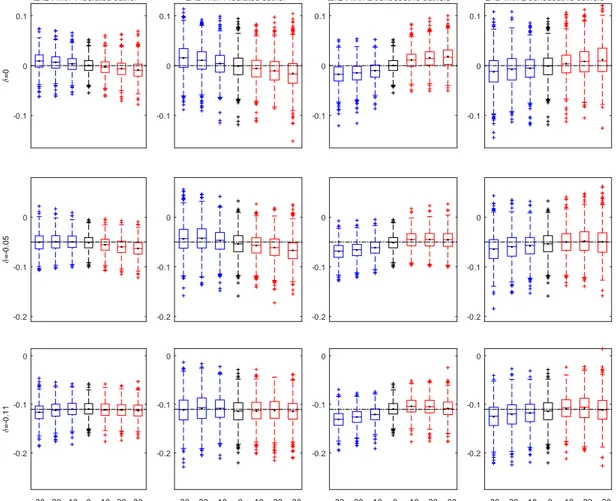
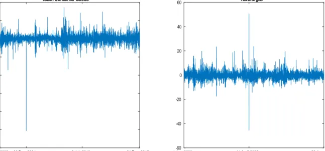
(17) test. Moreover, the parameters values of the two TGARCH models have been chosen to resemble the values usually encountered in real empirical applications and to make them somehow comparable, since their marginal variance and kurtosis are very similar. In particular, with these parameter sets, the marginal variance, the kurtosis and the 1st-order cross-correlation between squared and past returns are the following: Marginal variance Kurtosis 1st-order cross-correlation Parameter set 1 1 5:389 0:0647 Parameter set 2 1 5:727 0:135 Parameter set 3 0:9175 3:492 0 Since we are interested in the e¤ect of both the size and the sign of the outliers, we consider positive and negative outliers and we take the case of no outliers as a benchmark. In particular, the sizes of the outliers considered are the following: ! = f0; 10; 20; 30; 40; 50g. For each model, we generate 1000 independent samples. of size T = 1000.2 Then we contaminate each sample, …rst, with k = 1 isolated outlier of size ! at time t = T =2 and second, with k = 2 consecutive outliers of the same size but opposite signs placed at t = fT =2; T =2 + 1g. For instance, we contaminate with a negative outlier (! =. 10) at time t = 500 and a second one positive (! = 10) at time. t = 501 and then we repeat the experiments by contaminating …rst with a positive outlier (! = 10) at time t = 500 and a second one negative (! =. 10) at time t = 501. Then,. we repeat this procedure with each size of the outlier considered. For each replicate, we compute the estimates of the parameters (. 0;. ; ; ) by the three methods explained. above and we also compute their average over all replicates. For QML and QML-t estimates, we also compute, for each replicate, the asymptotic standard deviation of each estimator and the corresponding t-ratios to test for the signi…cance of each parameter. For comparison purposes, the LAD estimates are corrected by the corresponding scale factor M. 3.2. 1=2. (see Section 2.4). Moreover, for QML-t, the parameter. is also estimated.. Simulation results on estimation. As we are interested in the possible e¤ect of the outliers on the leverage e¤ect, we focus our discussion on the Monte Carlo results for the parameter . Actually, our results for 2. The results for T = f500, 5000g; not displayed to save space, are available upon request.. 17.

(18) the parameters. 0,. and. (not displayed here to save space) resemble those obtained in. Carnero et al. (2007, 2012) for symmetric GARCH models. In particular, QML always overestimates. 0. and underestimates. patches, and it overestimates. in the presence of outliers, either isolated or in. if there are two consecutive outliers. On the other hand,. QML-t is robust to one isolated outlier without losing the good properties of QML for uncontaminated series, but it fails to be robust to patches of big outliers, especially when estimating parameters. and . Moreover, we have also checked that the sign of. the outliers does not make a great di¤erence on estimating the parameters. 0,. and ;. it is only the magnitude of the outlier rather than its sign what makes the di¤erence. However, as Figures 2 and 3 will show, this is not the case when estimating the leverage parameter , where the sign of the outliers is essential. Figure 2 displays, in its left-hand side panels, the Box-plots of the QML estimates of for the three models considered (one for each row) in series contaminated with one single outlier of size ! for all the sizes considered, from the most negative value (! =. 50). to the highest positive one (! = 50). The central panels and the right-hand side panels of Figure 2 display the same plots for the QML-t and LAD estimates, respectively. Figure 3 displays similar Box-plots to those in Figure 2 but for series contaminated with two consecutive outliers of the same magnitude but opposite sign for all the outlier sizes considered. In particular, the labels in the x-axis of these plots represent the sign and size of the …rst outlier, being the 2nd one of the same magnitude but opposite sign. For instance, the Box-plot labelled as “ 50” represents the distribution of the 1000 estimated values of. from 1000 series contaminated with two consecutive outliers, namely. f 50; 50g, placed at t = f500; 501g, while the Box-plot labelled as “50”corresponds to the estimated values of. from 1000 series contaminated with two consecutive outliers,. namely f50; 50g, placed at t = f500; 501g. Several conclusions emerge from these …gures. First, QML is not robust to the presence of moderate-large outliers, as expected: both the bias and dispersion of QML estimates of increase with the size of the outliers. Actually, in the presence of moderatelarge outliers, the estimates can take any value within the admissible parameter space,. 18.

(19) Figure 2: Boxplots of estimated isolated outlier QM L with 1 isolated outlier. with QML, QML-t and LAD in the presence of one QM L-t with 1 isolated outlier. LAD with 1 isolated outlier. 0.5. 0.5. 0. 0. 0. -0.5. -0.5. -0.5. -1. -1. -1. 0.5. 0.5. 0.5. 0. 0. 0. -0.5. -0.5. -0.5. -1. -1. -1. 0.5. 0.5. 0.5. 0. 0. 0. -0.5. -0.5. -0.5. =-0.11. =-0.05. =0. 0.5. -1. -1 -50 -40 -30 -20 -10 0. 10 20 30 40 50. Size of outlier. -1 -50 -40 -30 -20 -10. 0. 10 20 30 40 50. Size of outlier. 19. -50 -40 -30 -20 -10. 0. 10 20 30 40 50. Size of outlier.

(20) Figure 3: Boxplots of estimated consecutive outliers QML with 2 consecutive outliers. with QML, QML-t and LAD in the presence of two QML-t with 2 consecutive outliers. LAD with 2 consecutive outliers. 0.5. 0.5. 0. 0. 0. -0.5. -0.5. -0.5. -1. -1. -1. 0.5. 0.5. 0.5. 0. 0. 0. -0.5. -0.5. -0.5. -1. -1. -1. 0.5. 0.5. 0.5. 0. 0. 0. -0.5. -0.5. -0.5. =-0.11. =-0.05. =0. 0.5. -1. -1 -50 -40 -30 -20 -10 0. 10 20 30 40 50. Size of outlier. -1 -50 -40 -30 -20 -10. 0. 10 20 30 40 50. Size of outlier. 20. -50 -40 -30 -20 -10. 0. 10 20 30 40 50. Size of outlier.

(21) rendering QML unreliable. Moreover, in models with leverage e¤ect ( 6= 0), the presence of one isolated outlier of either sign pushes QML estimate of. towards zero and. hence could hide true leverage e¤ect. This result agrees with the conclusions in Carnero et al (2016) regarding the identi…cation of leverage based on the cross-correlogram between past returns and current squared returns. Another remarkable feature is that, in general, two consecutive outliers are more harmful in QML than one isolated outlier of the same magnitude. Comparing Figures 2 and 3, we can see that, for a given model, both the bias and the interquartile range of QML estimates are always larger in the presence of two consecutive outliers than in the presence of one isolated outlier of the same size. However, the e¤ect of two consecutive outliers on QML estimates of. clearly. depends on the sign of the …rst outlier. If this is negative, QML underestimates. and. so it could yield spurious asymmetries (in models with no leverage) or it could overestimate the magnitude of the true leverage. By contrast,. is overestimated in series. contaminated with two consecutive outliers where the the 1st one is positive. Hence, in this case, QML could estimate spurious asymmetries (in models with no leverage) or it could either estimate asymmetries of the wrong sign or even no asymmetries in models with true leverage e¤ect. Again, this agrees with the results in Carnero et al. (2016) regarding the impact of consecutive outliers in the identi…cation of the leverage e¤ect. Figures 2 and 3 also show that both QML-t and LAD always outperform QML in the presence of outliers, as expected. Moreover, in the presence of one isolated outlier, both estimators perform quite well, even if the outlier is very large. However, they become slightly downward biased in the presence of two big consecutive outliers with the …rst one being negative. By contrast, when there are no outliers, QML is the best one, as expected, whereas LAD is the worst. Noticeably, QML-t does not lose much e¢ ciency with respect to QML in this case; a similar …nding is reported in Muler and Yohai (2008) for standard GARCH models. In order to better appreciate the di¤erences between QML-t and LAD, in Figure 4 we compare in more detail the results from these two estimators for some selected outlier sizes, namely ! = f0; 10; 20; 30g. As we can see, QML-t outperforms LAD in all cases, but in the presence of two consecutive outliers, it still su¤ers from some. biases, especially if the 1st outlier is negative. Moreover, in models with no leverage or even with low leverage, the presence of two consecutive outliers, being the …rst one. 21.

(22) positive, pushed QML-t estimated. upwards leading to a possible erroneous detection. of inverse leverage. Hence, there is still place to improve robustness in the estimation of asymmetric GARCH-type models, a topic that is left for further research.. 3.3. Simulation results on signi…cance tests. In this section we analyze the empirical properties of both the t-test and LR test using the standard rejection regions (11) and (12), respectively, to test H0 : H1 :. = 0 against. 6= 0: We only perform this analysis with the two likelihood-based estimators,. namely QML and QML-t. In all cases, the nominal size considered is 5%: In order to assess the empirical size of both tests, we simulated 1000 independent samples of size T=1000 of an AVGARCH (Parameter set 3) and, for each sample, we …tted a TGARCH model, by both QML and QML-t, and computed the corresponding t-ratio and loglikelihood. To calculate the LR statistic, we also …tted an AVGARCH and compare its log-likelihood with that of the …tted TGARCH. On the other hand, to analyze the empirical power of the tests, we simulated 1000 independent samples of size T=1000 of a TGARCH with Parameter set 2 ( =. 0:11) and, for each sample, we proceed. as before. We have also performed the same experiments with a TGARCH model with Parameter set 1 ( =. 0:05) obtaining similar conclusions.. Figure 5 compares the empirical size of the t test (left-hand side panels) and the LR test (right-hand side panels) based on both QML and QML-t estimates of TGARCH models contaminated with 1 isolated outlier (top panels) and with two consecutive outliers (bottom panels). That is, it represents the proportion of rejections under the null (H0 :. = 0), based on 5% critical value of t and LR tests using the standard. rejection regions (11) and (12), respectively. The main conclusions we can draw from this …gure are as follows. As expected, both the LR and t-test based on QML-t are always more robust to outliers than those based on QML. Moreover, as the outlier size increases, the tests based on QML become more oversized, i.e., they erroneously reject the null more often that they should and so they tend to identify spurious leverage. This problem is especially remarkable in the LR test, which could reach an over-rejection as huge as 80% in the presence of outliers of size larger than 15. By contrast, the tests. 22.

(23) Figure 4: Boxplots of estimated and two consecutive outliers. LAD with 1 isolated outlier. QML-t with 2 consecutive outliers. LAD with 2 consecutive outliers. 0.1. 0.1. 0.1. 0.1. 0. 0. 0. 0. -0.1. -0.1. -0.1. -0.1. 0. 0. 0. 0. -0.1. -0.1. -0.1. -0.1. -0.2. -0.2. -0.2. -0.2. 0. 0. 0. 0. -0.1. -0.1. -0.1. -0.1. -0.2. -0.2. -0.2. -0.2. =-0.11. =-0.05. =0. QML-t with 1 isolated outlier. with QML-t and LAD in the presence of one isolated. -30 -20 -10. 0. 10 20 30. Size of outlier. -30 -20 -10. 0. 10. 20. 30. -30 -20 -10. Size of outlier. 0. 10. Size of outlier. 23. 20. 30. -30 -20 -10. 0. 10. Size of outlier. 20. 30.

(24) based on QML-t keep the nominal size quite well and even better in the presence of 2 outliers than in the presence on 1 isolated outlier. It is also worth mentioning that, even with no outliers, the t-test does not reach the nominal size 5%. This could be related to the warning of Francq and Zakoian (2010), mentioned in Section 2.5, regarding the inappropriateness of the standard rejection region (11) in GARCH settings. This topic is out of the scope of this paper but deserves further research. Figure 6 compares the empirical powers of the t test (left-hand side panels) and the LR test (right-hand side panels) based on both QML and QML-t estimates of TGARCH models contaminated with 1 isolated outlier (top panels) and with two consecutive outliers (bottom panels). That is, this …gure displays, for each test, the relative frequency of rejection of the hypothesis H0 :. = 0 (no leverage) on 1000 independent realizations. of length T = 1000 of the TGARCH model with parameter. =. 0:11 (Parameter set. 2). This …gure shows that, in terms of power, both the LR and t-test based on QML-t are again more robust to outliers than those based on QML, as expected. The power of the tests based on QML decreases rapidly with the size of the outlier, although the loss of power is not that big in the LR test, which keeps the power around 80% when it is based on QML, even in the presence of huge outliers. However, the loss of power due to outliers of the t-test based on QML is dramatic. By contrast, the power of the tests based on QML-t is around 1 in all cases, regardless of the size, the sign and the amount of the outliers in the sample.. 4. Empirical application. In this section we illustrate the previous results by …tting both the AVGARCH and the TGARCH models to two series of daily returns from di¤erent markets by using the estimation methods describe above. For each series and estimated model, we check whether the leverage parameter is signi…cant or not by applying both the t-ratio and LR tests. The two series analyzed have been chosen to represent the possible e¤ects than one isolated outlier and two consecutive outliers have on the inferential statistics.. 24.

(25) Figure 5: Monte Carlo size. Proportion of rejections based on 5% critical value of t and LR tests under H0 : = 0 t-ratio test 1. LR test 1. QML. One single outlier. QML-t 0.8. 0.8. 0.6. 0.6. 0.4. 0.4. 0.2. 0.2. Two consecutive outliers. 0 -50. 0. 0 -50. 50. 1. 1. 0.8. 0.8. 0.6. 0.6. 0.4. 0.4. 0.2. 0.2. 0 -50. 0. 0 -50. 50. Size of the outlier(s). 25. 0. 0 Size of the outlier(s). 50. 50.

(26) Figure 6: Monte Carlo power. Proportion of rejections based on 5% critical value of t and LR tests under H1 : = 0:11 t-ratio test. LR test. 1. 1. One single outlier. QML QML-t 0.8. 0.8. 0.6. 0.6. 0.4. 0.4. 0.2. 0.2. Two consecutive outliers. 0 -50. 0. 0 -50. 50. 1. 1. 0.8. 0.8. 0.6. 0.6. 0.4. 0.4. 0.2. 0.2. 0 -50. 0. 0 -50. 50. Size of the outlier(s). 26. 0. 0 Size of the outlier(s). 50. 50.

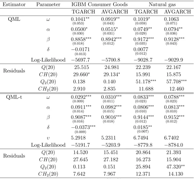
(27) 4.1. Data description and dynamic properties. The series analyzed are daily close-to-close returns of the Spain IGBM Consumer Goods index observed from June 3, 2002 to December 31, 2015, comprising 3398 observations, and daily open-to-open returns of futures contracts of Natural gas from January 4, 2000 to June 28, 2013, comprising 3368 observations3 . In both cases, the returns are computed as yt = 100. (log(Pt ). log(Pt 1 )); where Pt is the closing price at time t for. the IGBM series but it represents the open price at date t for the Natural gas. The two series are plotted in Figure 7. As we can see, they both display volatility clustering and some occasional extreme values that could be regarded as outliers. For instance, the IGBM returns exhibit several extreme observations, the largest one corresponding to December 30, 2004, when the index drops by. 25:3%. The Natural gas returns exhibit. two extreme consecutive observations, the …rst one positive and the second one negative, of magnitudes about 12 times the standard deviation of the series. These outliers are due to large changes in the open price of the Natural gas on the 13th, 14th and 15th of April 2006, with values of 6.78, 11.26 and 7.15 dollars, respectively. Table 1 contains descriptive statistics of the two series considered, as well as the Jarque-Bera and the Ljung-Box Q(20) test statistics, the heteroscedastic-corrected Qc (20) test statistic proposed by Diebold (1988), and the test statistic CH(20); proposed by Cumby and Huizinga (1992) which is also robust to conditional heteroscedasticity. We also include the values of the statistics Q and CH applied to the squared returns, denoted by Q2 (20) and CH2 (20), respectively, to test for conditional heteroscedasticity. As expected, both series exhibit excess kurtosis and the Jarque-Bera test for Normality always rejects the null. The values of Qc (20) and CH(20) never reject the null at 5% signi…cance level, suggesting that both returns are uncorrelated, as expected. Surprisingly, the values of Q2 (20) and CH2 (20) are not signi…cant for the IGBM series, suggesting that its conditional variance is constant over time, while the values of these test statistics are signi…cant at 1% for the Natural gas, indicating strong evidence of conditional heteroscedasticity.. 3. The data for the IGBM Consumer Goods index was downloaded from www.invertia.com and the corresponding one for Natural gas was obtained from the additional …les in Kristoufek (2014).. 27.

(28) Figure 7: Daily returns for IGBM Consumer Goods index and Natural gas IGBM Consumer Goods. 10. 60. Natural gas. 5 40 0 20 -5. 0. -10. -15 -20 -20 -40 -25. -30 4 Jun. 2002. 30 Dec. 2004. 9 Jul. 2010. -60 4 Jan. 2000. 31 Dec. 2015. 28. 14 April 2006. 28 Jun. 2013.

(29) Table 1: Descriptive statistics of the returns. Statistic IGBM Consumer Goods Natural gas Mean 0:0439 0:0149 Std.Dev. 1:3320 3:7653 Skewness 2:0142 0:7462 Kurtosis 44:542 21:765 Jarque-Bera 246630 4973 Sample size 3398 3368 48:547 Q(20) 37:537 Qc (20) 28:989 18:593 CH(20) 28:956 18:975 Q2 (20) 2:9310 631:56 CH2 (20) 23:119 75:94 ; ; : statistically signi…cant at 10%, 5% and 1% respectively. 29.

(30) Figure 8 displays, in its …rst row, the correlograms of the returns with the corrected 95% con…dence bands proposed by Diebold (1988) for conditionally hereroscedastic series. These bands are wider than the usual Barlett bands and show no evidence of autocorrelated returns. The correlogram of squared returns, displayed in the 2nd row of Figure 8, suggests no correlation in the squared returns of IGBM, looking like the typical correlogram of a white noise series and con…rming the previous result on the tests Q2 (20) and CH(20). Nevertheless, it should be noticed that the pattern of this correlogram can also be due to the harmful e¤ect of one isolated outlier on conditionally heteroscedastic series; see Carnero et al. (2007). On the other hand, for the Natural gas, we can see the typical pattern of the correlogram of the squared observations in the presence of two consecutive outliers, that is, a very high positive and signi…cant 1st order correlation while the others are pushed downwards towards zero; see Carnero et al. (2007). However, when the robust autocorrelations of squares proposed by Teräsvirta and Zhao (2011) are computed (see the 3rd row of Figure 8), another picture comes up. For both, the IGBM and the Natural gas, all these correlations become signi…cantly di¤erent from zero, suggesting that the conditional variances of both returns are not constant over time, as expected, and con…rming that the patterns of the sample autocorrelations are due to the presence of outliers. Finally, the last two rows of Figure 8 display the sample cross-correlations between past and squared returns and their robust counterparts, respectively. The latter are computed using the proposal in Carnero et al. (2016) based on applying the Ramsay weighting scheme to the sample variances and cross-covariances. Again, the picture changes depending on whether we look at the sample or the robust cross-correlations. For the IGBM returns, the sample cross-correlations suggest no leverage e¤ect. By contrast, most of the robust cross-correlations are negative suggesting possible leverage e¤ect in this series. As discussed in Carnero et al. (2016), this is the expected pattern due to one isolated outlier, which biases all sample cross-correlations towards zero hiding true leverage. On the other hand, for the Natural gas, the patterns are quite di¤erent,. 30.

(31) Figure 8: Correlograms of returns and squared returns and cross-correlograms between lagged returns and squared returns IGBM Consumer Goods. r(h). 0.1 0. 0. -0.1. -0.1. 2. r (h). 0. 5. 10. 15. 20. 0.4. 0.4. 0.2. 0.2. 0. 2. Robust r (h). 5. 10. 15. 20. 0.4. 0.4. 0.2. 0.2. 0. 0 0. (h). 0. 5. 10. 15. 20. 0. 5. 10. 15. 20. 0. 5. 10. 15. 20. 0. 5. 10. 15. 20. 0. 5. 10. 15. 20. 0 0. 5. 10. 15. 20. 0.1. 0.1. 0. 0. -0.1. -0.1. r. 12. Natural gas. 0.1. Robust r. 12. (h). 0. 5. 10. 15. 20. 0.1. 0.1. 0. 0. -0.1. -0.1 0. 5. 10. 15. 20. Lag. Lag. 31.

(32) whereas all the robust cross-correlations are around zero, indicating no leverage e¤ect, the 1st sample cross-correlation is pushed upwards to a signi…cant positive value, suggesting inverse leverage e¤ect (positive relationship between volatility and past returns). Again, this is the expected pattern due to the presence of two consecutive outliers, being the …rst one positive; see Carnero et al. (2016). Therefore, the inverse leverage e¤ect found in the Natural gas by some authors (see Kristoufek (2014) and the references therein) could be an artifact due to the misleading e¤ect of outliers.. 4.2. Estimating and testing for leverage e¤ect. We describe below the results from estimating the TGARCH and AVGARCH models to the two return series described above. Since the results in Section 3 suggest a better performance of QML-t over LAD and the computation of the standard errors of the latter is cumbersome, we focus our comparison on QML and QML-t, although the estimated leverage parameter by LAD will be also commented. Table 2 displays the estimation results obtained by QML and QML-t as well as some diagnostics based on the residuals, b "t = yt =bt , where bt is the estimated volatility for each model. The. estimation has been carried out with the Oxford MFE Toolbox for Matlab, taking into account the reparametrization used in this package (see Appendix A) in order to compute the estimated parameter values and their corresponding standard errors.4 As we can see, there are remarkable di¤erences between the results obtained for the two returns series and, for each series, there are also some di¤erences between both estimation methods that are worth mentioning. Since we are interested in the e¤ects of outliers on estimating and testing the leverage e¤ect, our comments will be focused on the leverage parameter . For the IGBM series, we can see that, regardless of the estimation method, the parameter. in the TGARCH model is estimated negative, as it is expected if there is leverage e¤ect. The LAD estimate is also negative (bLAD =. 0:0229). However, the leverage coe¢ cient is not statistically signi…cant when the. 4. To check for the robustness of our results, we have repeated the estimation by QML and QMLt in Stata, obtaining similar results. We have also estimated EGARCH models leading to similar conclusions.. 32.

(33) Table 2: Estimation of the TGARCH and AVGARCH models with QML and QML-t Estimator. Parameter. QML. !. IGBM Consumer Goods Natural gas TGARCH AVGARCH TGARCH AVGARCH 0:1041 0:0919 0:1019 0:1063 (0:053). (0:043). (0:059). (0:071). 0:0500. 0:0515. 0:0749. 0:0794. 0:8858. 0:8942. 0:9172. 0:9128. (0:030). (0:018). (0:031). (0:012). 0:0171. Residuals. QML-t. !. 5697:7 25:515 29:660 0:138 2:910. (0:035). (0:036). (0:043). 0:0077 (0:012). (0:013). Log-Likelihood Q(20) CH(20) Q2 (20) CH2 (20). (0:029). 5700:8 24:981 29:134 0:140 2:835. 9028:7 22:239 15:991 51:178 11:688. 9029:9 22:167 15:875 57:708 12:460. 0:0292. 0:0310. 0:0833. 0:0788. 0:0911. 0:0982. 0:0806. 0:0813. 0:9087. 0:9016. 0:9144. 0:9152. (0:009). (0:014). (0:016). (0:011). (0:015). (0:018). 0:0373. (0:010). (0:012). (0:023). (0:010). (0:012). 0:0185. (0:007). (0:009). 5:2918 Log-Likelihood 5191:7 Q(20) 14:520 Residuals CH(20) 27:645 Q2 (20) 0:113 CH2 (20) 7:642 ; ; : statistically signi…cant at. (0:023). 5:2311 6:7494 6:7402 5203:9 8779:8 8784:0 15:451 20:864 21:393 27:182 16:273 15:904 0:151 25:894 47:320 7:967 12:371 14:130 10%, 5%, and 1%, respectively. 33.

(34) QML-based t-ratio test is applied but becomes signi…cant when QML-t is used. In particular, the values (and p-values) of the t-statistic are. 1:330 (0:1836) and. 4:276. (0:000), respectively. Meanwhile, the values (and p-values) of the LR test statistic for H0 :. = 0 (AVGARCH) against H1 :. 6= 0 (TGARCH) are 6:248 (0:0124) and 24:356. (0:000) when the models are estimated by QML and QML-t, respectively, con…rming that. is signi…cant when QML-t is used but it is not longer signi…cant at 1% when. QML is applied. This result agrees with our discussion in Section 3 where we show that a single isolated outlier (like the one existing in the IGBM series) biases the QML estimated. towards zero and could hide true leverage. Then, it seems that, in this case,. QML-t is more reliable than QML suggesting that there is leverage e¤ect in the IGBM returns, although this is hidden by the huge return observed on December 30, 2004, when the model is estimated by QML. For the Natural gas series, the parameter is estimated positive by both QML and QML-t and also by LAD (bLAD = 0:0217), suggesting inverse leverage e¤ect. However, its statistical signi…cance also depends on the estimator used as well as the test statistic chosen. For this series, the values (and p-values) of both the t-ratio and LR test statistics. are 0:636 (0:5247) and 2:377 (0:123), respectively, when QML is used, indicating no evidence of leverage e¤ect at any reasonable signi…cance level. But, when the model is estimated using QML-t, the values (and p-values) of these two test statistics are 2:550 (0:0108) and 8:458 (0:0036), respectively, showing evidence of inverse leverage e¤ect at 5% signi…cance level (or even at 1% if the LR test is selected). This somehow surprising result could be related to our …ndings in Section 3, where we show that QML-t could be still biased in the presence two big consecutive outliers, with the estimated. being. pushed upwards if the …rst of these outliers is positive, as it is the case in the Natural gas series. Therefore, we should be very careful in concluding that there is actually inverse leverage e¤ect in this series, as this could be a misleading e¤ect caused by the two consecutive extreme observations present in this series. Finally, it is also worth mentioning that the thickness parameter. of the Student error distribution in QML-t,. indicates fat tails in both returns. When looking at residuals diagnostics, as expected, the values of the test statistics Q2 (20) and CH2 (20) for remaining autocorrelation in the squared residuals, have been reduced remarkably in all estimated models, as compared to their values for the. 34.

(35) returns displayed in Table 1. Only for the Natural gas, the values of Q2 (20) remain signi…cant at 1% when the two models are estimated by QML. However, when QML-t is used, both statistics Q2 (20) and CH2 (20) are not longer signi…cant for the TGARCH model, suggesting that this model has been able to properly capture the dynamics in the conditional variance of the returns. To further illustrate how the potential outliers can bias the estimation and testing of the leverage e¤ect, we consider a rolling window scheme of size T = 1000 through the whole sample, starting at point t = 1 and moving forwards up to covering the last 1000 observations of the full sample. For the IGBM and the Natural gas series, this amounts to analyzing 2398 and 2368 subsamples, respectively, covering periods of di¤erent volatilities and types and sizes of outliers, according to the following steps: 1. Select the 1st subsample for IGBM (04/06/2002 - 31/07/2006) and for Natural gas (04/01/2000 - 9/01/2004), estimate the parameter. by the three methods. considered (QML, QML-t and LAD) and compute, for QML and QML-t, the corresponding t-ratio and LR test statistics for these subseries. 2. Delete the 1st observation, add a new observation at the end of the subsample and re-estimate the model and test again for leverage. 3. Repeat the process until we reach the end of the full samples, where we cover the last subsamples for IGBM (26/01/2012 - 31/12/2015) and Natural gas (23/06/2009 - 28/06/2013). Figure 9 plots, in its …rst row, the estimated values of. across the rolling window for. the two series considered and for the three estimation methods applied, i.e., it plots the values of bQM L , bQM L t and bLAD for each of the 2398 subseries of the IGBM series (left-. hand side panel) and for each of the 2368 subseries of the natural gas series (right-hand side panel). As a benchmark, the zero line is also displayed to account for no leverage.. Similarly, Figure 9 plots the corresponding p-values of both the t-ratio (2nd row) and the LR (3rd row) tests to test H0 :. = 0 against H0 :. 6= 0. The horizontal line. represents the 5% signi…cance level and consequently, those subsamples with p-values below this line are those where the leverage e¤ect is signi…cant at 5% signi…cance level.. 35.

(36) Figure 9: Leverage parameter in a TGARCH model estimated with subsamples of size T = 1000 using a rolling window of both the IGBM Consumer Goods index and Natural gas daily returns (top panels) and the corresponging p-values of the t-ratio and LR test statistics to test for the statistical signi…cance of . IGBM Consumer Goods. Estimated. 0.1. 0. 0. -0.1. -0.1. p-values t-ratio. 0. 500. 1000. 1500. 2000. 0. 1. 1. 0.5. 0.5. 0. 500. 1000. 1500. 2000. 0. 500. 1000. 1500. 2000. 0. 500. 1000. 1500. 2000. QML QML-t. 0 0. p-values LR. Natural Gas. 0.1. QML QML-t LAD. 500. 1000. 1500. 2000. 1. 1. 0.5. 0.5. 0. 0 0. 500. 1000. 1500. 2000. Subseries. Subseries. 36.

(37) Several conclusions emerge from this …gure. First, we observe how extreme observations can bias the estimated leverage parameter and the corresponding test statistics and could lead to a wrong conclusion about the sign and magnitude of the leverage e¤ect. As expected, the QML estimated values of. present several sharp drops and rises which. do not appear in their robust counterparts. These sharp changes are usually due to the entrance and/or an exit of outlying observations in the corresponding subsample. For instance, in the IGBM series, the exit of the observation in December 30, 2004, where the index sustained its largest drop (y642 = 25:33), conveys a sudden fall in bQM L from a positive value to a negative value around. 0:035 (see the graph in the top left-hand. side panel). Noticeably, for the …rst subseries corresponding at the beginning of the full sample, i.e., for those including that isolated outlier, bQM L is always positive but. not signi…cant at any reasonable signi…cance level, as judged by the t-ratio test (see the corresponding p-values displayed in the left panel in the 2nd row of Figure 9). Moreover, for these subsamples, there are big di¤erences between bQM L and the robust estimates, bQM L t and bLAD , which are both both mainly negative and very similar to each other. Actually, when QML-t is used, the p-values of both signi…cance tests show that. is. statistically signi…cant for several subsamples, indicating the presence of leverage e¤ect.. Recall that, according to our results in Section 3, these di¤erences are expected in the presence of one isolated outlier, which seems to be the cause here of the upwards bias observed in bQM L , as compared to the robust estimators.. It is also worth noting that, when we look at the patterns after the exit of that. outlying negative observation of the IGBM index, i.e. when the subseries analyzed do not longer contain this outlier, the di¤erences between the three estimators (QML, QMLt and LAD) are considerably reduced, specially for the last subseries at the end of the sample. Actually, for these subseries, which are free from outliers (see the calm period in the IGBM returns displayed in Figure 7 at the end of the sample), we observe that, regardless of the estimator and the test statistics used,. is always estimated negative. and statistically signi…cant indicating the presence of leverage e¤ect. Again, this result agrees with our …ndings in Section 3 for the simulated series without outliers. When looking at the results for the Natural gas (right-hand side panels), we observe remarkable di¤erences among the three estimators considered, specially for the subseries located around the middle of the sample, i.e., those including the two huge consecutive. 37.

(38) outliers present in this series (y1566 = 50:73 and y1567 =. 45:41). In these cases, our. results in Section 3 show that even the robust estimators could still be slightly biased. In particular, when these two observations, the …rst one being positive and the next one negative, are in a subsample, we expect bQM L but also bQM L t to be upwards biased.. Another remarkable feature from the Natural gas results in Figure 9, is that the values of bQM L and bQM L t for the subseries at the end of the period (see the graph in the. top right-hand side panel), are very similar to each other but quite di¤erent from the values of bLAD : the former take negative values (standard leverage) whereas the latter estimate. > 0 (inverse leverage). This feature could be related to the fact that LAD. is underperforming if no outliers are present in the series, as discussed in Section 3.. Accordingly, for most of the subseries at the end of the period, neither the t-ratio nor the LR test statistics based on QML and QML-t reject the null, H0 :. = 0, in these. subseries. Therefore, we wonder whether the inverse leverage e¤ect found in the Natural gas returns by some authors (see, for example, Kristoufek (2014) and the references therein) could be due to the harmful e¤ect of these consecutive outliers. Alternatively, the patterns of the estimated parameters displayed in Figure 9 could be indicating that the leverage e¤ect is time-varying, as suggested by Bandi and Reno (2012), Yu (2012) and Jensen and Maheu (2014), but this is a di¤erent problem that is out of the scope of this paper.. 5. Conclusions. This paper has analyzed the e¤ects of outliers on the estimation and testing for the leverage e¤ect in the context of the TGARCH model. It is shown that, as expected, QML-t and LAD always outperform QML in the presence of outliers. Actually, one isolated outlier could lead QML to hide true leverage e¤ect whereas two consecutive outliers bias the QML estimated leverage in a direction that crucially depends on the sign of the …rst outlier. If this is negative (positive), QML underestimates (overestimates) the leverage parameter. Therefore, in these cases, QML could hide true leverage or estimate spurious asymmetries or asymmetries of the wrong sign. However, both robust estimators perform very well when there is one isolated outlier, but they are still slightly biased in the presence of patches of big outliers, leading, in some cases, to inaccurate. 38.

(39) estimates of the leverage coe¢ cient. In general, QML-t seems to outperform LAD because it is robust to moderate-big outliers without losing much e¢ ciency, as compared to QML, when there are no outliers. That is not the case for LAD, which performs much worse than QML with no outliers. These results are further illustrated with the empirical analysis of two return series from …nancial and energy markets, including one isolated negative outlier and two consecutive outliers, respectively.. 39.

(40) Appendix A. Parametrizations of the TGARCH(1,1) model There are several (equivalent) parametrizations of the TGARCH(1,1) model proposed in the econometric literature and also in the econometric software packages. Hence, in order to compare estimates and standard errors from di¤erent papers and/or di¤erent software packages, it is important to be very careful about which parametrization is being used in each case. The one we have adopted in this paper is taken from Rodríguez and Ruiz (2012) and it is given by the following equations: yt = t. =. 0. t. "t ;. jyt 1 j +. +. t 1. (A.1). + yt 1 :. Hence, the volatility equation (A.1) can be re-written as: ( if yt 0 + ( + ) yt 1 + t 1 t = ( ) yt 1 + t 1 if yt 0. 1. 0. 1. <0. :. (A.2). In turn, the original proposal in Zakoian (1994) de…nes the volatility as follows: t. =. 0. +. + + yt 1. yt. +. 1. (A.3). t 1;. where: yt+ = max(yt ; 0); yt = min(yt ; 0): Hence, the volatility equation (A.3) can be re-written as: ( + yt 1 + t 1 if yt 0+ t = yt 1 + t 1 if yt 0. 1. 0. 1. <0. :. (A.4). Therefore, comparing (A.2) and (A.4), the following relationship comes up between the parameters of both parametrizations: + = =. = 21 ( = 12 (. +. (). +. +. ) : ). +. He and Teräsvirta (1999) consider the same volatility speci…cation as Zakoian (1994), but they write it down in a slightly di¤erent way, namely t. =. 0. +. t 1f. +[. +. (1. I("t 1 )) +. 40. I("t 1 )] j"t 1 jg;. (A.5).

(41) where I("t 1 ) = Hence, taking into account that yt. 1. ( 1 if "t. 1. <0. 0 otherwise. =. t 1 "t 1. :. and sign(yt 1 ) = sign("t 1 ), the volatil-. ity equation (A.5) can be easily re-written as in (A.4). Another proposal, very similar to that in Rodríguez and Ruiz (2012), can be found in He et al. (2008), whose volatility equation is as follows =. t. 0. t 1f. +. Hence, taking into account that yt re-written as in (A.1) with. =. 1. +. j"t 1 j +. t 1 "t 1 ,. "t 1 g:. (A.6). the volatility equation (A.6) can be. = .. Finally, the MFE Toolbox for Matlab that we have used in our Monte Carlo experiments and empirical application, employs the following volatility equation for the TGARCH(1,1) model: t. =. 0. +. 1 jyt 1 j. 1 jyt 1 j. +. where I(yt. 1. < 0) =. I(yt. 1. < 0) +. ( 1 if yt. 1. <0. 0 otherwise. t 1;. (A.7). :. Hence, the volatility equation (A.7) can be re-written as: ( if yt 0 + 1 yt 1 + t 1 t = ( 1 + 1 ) yt 1 + t 1 if yt 0. 1. 0. 1. <0. :. (A.8). Therefore, comparing (A.2) and (A.8), the following relationships come up: + = =. 1 1. +. 1. (). = 1+ = 12. 1 2 1. :. 1. These relationships should be taken into account to properly compute the correct point ; ; )0 from the estimated parameters computed by the MFE Toolbox, namely (b 0 ; b 1 ; b; b1 ), and their asymptotic. estimates and standard errors of our parameters (. 0;. variance-covariance matrix.. Another parametrizations of the TGARCH(1,1) model are still possible; see, for. instance, Hentschel (1995).. 41.

(42) References [1] Andersen, T.G., Bollerslev, T., Diebold, F.X. and Ebens, H. (2001) The distribution of realized stock return volatility. Journal of Financial Economics 61, 43–76. [2] Ait-Sahalia, Y., Fan, J. and Li, Y. (2013) The leverage e¤ect puzzle: Disentangling sources of bias at high frequency. Journal of Financial Economics 109, 224–249. [3] Bandi, F. and Reno, R. (2012) Time-varying leverage e¤ects. Journal of Econometrics 169, 94–113. [4] Berkes, I. and Horvath, L. (2004) The e¢ ciency of the estimators of the parameters in GARCH processes. The Annals of Statistics 32, 633–655. [5] Black, R. (1976) Studies in stock price volatility changes, Proceedings of the 1976 Business Meeting of the Business and Economics Statistics Sections, American Statistical Association, 177–181. [6] Carnero, M.A., Peña, D. and Ruiz, E. (2007) E¤ects of outliers on the identi…cation and estimation of GARCH models. Journal of Time Series Analysis 28, 471–497. [7] Carnero, M.A., Peña, D. and Ruiz, E. (2012) Estimating GARCH volatility in the presence of outliers. Economics Letters 114, 86–90. [8] Carnero, M.A., Pérez, A. and Ruiz, E. (2016) Identi…cation of asymmetric conditional heteroscedasticity in the presence of outliers. SERIEs: Journal of the Spanish Economic Association 7, 179 –201. [9] Chkili, W., Hammoudeh, S. and Nguyen, D. (2014) Volatility forecasting and risk management for commodity markets in the presence of asymmetry and long memory. Energy Economics 41, 1–18. [10] Creal, D., Koopman, S. J. and Lucas, A. (2013) Generalized autoregressive score models with applications. Journal of Applied Econometrics 28, 777-795. [11] Cumby, R. and Huizinga, J. (1992) Testing the autocorrelation structure of disturbances in ordinary least squares and instrumental variables regressions. Econometrica 60, 185–195.. 42.

(43) [12] Diebold, F.X. (1988) Empirical Modeling of Exchange Rate Dynamics, SpringerVerlag. [13] Ding, Z., Granger, C. and Engle, R. (1993) A long memory property of stock market returns and a new model. Journal of Empirical Finance 1, 83–106. [14] Engle, R.F. (2011) Long term skewness and systematic risk. Journal of Financial Econometrics 9, 437–468. [15] Fan, J., Qi, L. and Xiu, D. (2014) Quasi-Maximum likelihood estimation of GARCH models with heavy-tailed likelihoods. Journal of Business and Economic Statistics 32, 178–191. [16] Francq, C. and J-M. Zakoian (2010) GARCH Models: Structure, Statistical Inference and Financial Applications. Wiley. [17] Francq, C. and J-M. Zakoian (2013) Optimal predictions of powers of conditionally heteroscedastic processes. Journal of the Royal Statististical Society B 75, 345–367. [18] Glosten, L.R., Jagannathan, R. and Runkle, D.E. (1993) On the relation between the expected value and the volatility of the nominal excess return on stocks. The Journal of Finance 48, 1779–1801. [19] Harvey, A. C. (2013) Dynamic Models for Volatility and Heavy Tails: With Applications to Financial and Economic Time Series. Cambridge University Press. [20] He, C. and Teräsvirta, T. (1999) Properties of moments of a family of GARCH processes. Journal of Econometrics 92, 173–192. [21] He, C., Silvennoinen, A. and Teräsvirta T. (2008) Parameterizing unconditional skewness in models for …nancial time series. Journal of Financial Econometrics 6, 208–230. [22] Hentschel, L. (1995) All in the family Nesting symmetric and asymmetric GARCH models. Journal of Financial Economics 39, 71–104.. 43.

(44) [23] Hibbert, A.M., Daigler, R.T. and Dupoyet, B. (2008) A behavioral explanation for the negative asymmetric return-volatility relation. Journal of Banking and Finance 32, 2254–2266. [24] Hill, J.B. (2015) Robust estimation and inference for heavy tailed GARCH. Bernoulli 21, 1629–1669. [25] Huang, D., Wang, H. and Yao, Q. (2008) Estimating GARCH models: when to use what? Econometrics Journal 11, 27–38. [26] Hwang, S. and Basawa, I. (2004) Stationarity and moment structure for Box-Cox transformed threshold GARCH(1,1) processes. Statistics & Probability Letters 68, 209–220. [27] Jensen, M.J. and Maheu, J.M. (2014) Estimating a semiparametric stochastic volatility model with a Dirichlet process mixture. Journal of Econometrics 178, 523–538. [28] Kristoufek, L. (2014) Leverage e¤ect in energy futures. Energy Economics 45, 1–9. [29] Laurent, S., Lecourt, C. and Palm, F.C. (2016) Testing for jumps in conditionally Gaussian ARMA-GARCH models, a robust approach. Computational Statistics & Data Analysis 100, 383–400. [30] Mendes, B. (2000) Assessing the bias of maximum likelihood estimates of contaminated garch models. Journal of Statistical Computation and Simulation 67, 359–376. [31] Muler, N. and Yohai, V. (2008) Robust estimates for GARCH models. Journal of Statistical Planning and Inference 138, 2918–2940. [32] Nelson, D.B. (1991) Conditional heteroskedasticity in asset returns: a new approach. Econometrica 59, 347–370. [33] Newey, W. K. and Steigerwald, D.G. (1997) Asymptotic bias for quasi-maximumlikelihood estimators in conditional heteroskedasticity. Econometrica 65, 587–599.. 44.

(45) [34] Pan, J., Wang H. and Tong H. (2008) Estimation and tests for power-transformed and threshold GARCH models. Journal of Econometrics 142, 352–378. [35] Peng, L. and Yao, Q. (2003) Least absolute deviations estimation for ARCH and GARCH models. Biometrika 90, 967–975. [36] Rodríguez, M.J. and Ruiz E. (2012) GARCH models with leverage e¤ect: di¤erences and similarities. Journal of Financial Econometrics 10, 637–668. [37] Sakata, S. and White, H. (1998) High breakdown point conditional dispersion estimation with application to S&P 500 daily returns volatility. Econometrica 66, 529–567. [38] Schwert, G.W. (1989) Why does stock market volatility change over time? Journal of Finance 45, 1129–1155. [39] Sentana, E. (1995) Quadratic ARCH Models. Review of Economic Studies 62, 639– 661. [40] Straumann, D. and Mikosch T. (2006) Quasi-maximum-likelihood estimation in heteroskedastic time series: A stochastic recurrence equations approach. Annals of Statistics 34, 2449–2495. [41] Taylor, S.J. (1986) Modelling Financial Time Series. Wiley. [42] Teräsvirta, T. and Zhao Z (2011) Stylized facts of return series, robust estimates and three popular models of volatility. Applied Financial Economics 21, 67–94. [43] Wintenberger, O. (2013) Continuous invertibility and stable QML estimation of the EGARCH(1,1) model. Scandinavian Journal of Statistics 40, 846–867. [44] Yu, J. (2012) A semiparametric stochastic volatility model. Journal of Econometrics 167, 473–482. [45] Zakoian, J.M. (1994) Threshold heteroskedastic models. Journal of Economic Dynamics and Control 18, 931–955.. 45.