Exploring Cross layer power management for PGAS applications on the SCC platform

Texto completo

(1)Exploring Cross-layer Power Management for PGAS Applications on the SCC Platform Marc Gamell [email protected]. Advisor: Ivan Rodero Open University of Catalonia (UOC) 2011-2012.

(2) Contents 1 Introduction. 2. 1.1. Motivation. . . . . . . . . . . . . . . . . . . . . . . . . . . . . . . . . . . . . . . . .. 2. 1.2. Objectives . . . . . . . . . . . . . . . . . . . . . . . . . . . . . . . . . . . . . . . . .. 3. 1.3. Contributions . . . . . . . . . . . . . . . . . . . . . . . . . . . . . . . . . . . . . . .. 3. 1.4. Planning . . . . . . . . . . . . . . . . . . . . . . . . . . . . . . . . . . . . . . . . . .. 4. 1.5. Organization . . . . . . . . . . . . . . . . . . . . . . . . . . . . . . . . . . . . . . .. 4. 2 Single-chip Cloud Computer background. 6. 2.1. Many-core motivation . . . . . . . . . . . . . . . . . . . . . . . . . . . . . . . . . .. 6. 2.2. Intel SCC’s architecture overview . . . . . . . . . . . . . . . . . . . . . . . . . . . .. 6. 2.3. Other existing many-cores . . . . . . . . . . . . . . . . . . . . . . . . . . . . . . . .. 7. 2.4. Memory . . . . . . . . . . . . . . . . . . . . . . . . . . . . . . . . . . . . . . . . . .. 8. 2.5. Mesh . . . . . . . . . . . . . . . . . . . . . . . . . . . . . . . . . . . . . . . . . . . .. 9. 2.6. SCC’s message passing library . . . . . . . . . . . . . . . . . . . . . . . . . . . . . .. 9. 2.7. Rocky-Lake (SCC board) architecture . . . . . . . . . . . . . . . . . . . . . . . . .. 9. 2.8. Power management capabilities . . . . . . . . . . . . . . . . . . . . . . . . . . . . .. 9. 2.8.1. Power monitoring . . . . . . . . . . . . . . . . . . . . . . . . . . . . . . . . .. 3 Unified Parallel C background. 12 13. 3.1. PGAS . . . . . . . . . . . . . . . . . . . . . . . . . . . . . . . . . . . . . . . . . . .. 13. 3.2. UPC overview . . . . . . . . . . . . . . . . . . . . . . . . . . . . . . . . . . . . . . .. 13. 3.3. Berkeley UPC . . . . . . . . . . . . . . . . . . . . . . . . . . . . . . . . . . . . . . .. 14. 4 Related work. 15. 4.1. Layered power management research . . . . . . . . . . . . . . . . . . . . . . . . . .. 15. 4.2. Many-core research . . . . . . . . . . . . . . . . . . . . . . . . . . . . . . . . . . . .. 16. i.

(3) ii. CONTENTS 4.3. PGAS research . . . . . . . . . . . . . . . . . . . . . . . . . . . . . . . . . . . . . .. 5 Profiling of UPC applications. 16 18. 5.1. Methodology . . . . . . . . . . . . . . . . . . . . . . . . . . . . . . . . . . . . . . .. 18. 5.2. NAS Parallel Benchmarks . . . . . . . . . . . . . . . . . . . . . . . . . . . . . . . .. 19. 5.2.1. NAS FT kernel . . . . . . . . . . . . . . . . . . . . . . . . . . . . . . . . . .. 20. 5.2.2. NAS MG kernel . . . . . . . . . . . . . . . . . . . . . . . . . . . . . . . . .. 24. 5.2.3. NAS EP kernel . . . . . . . . . . . . . . . . . . . . . . . . . . . . . . . . . .. 28. 5.3. Sobel . . . . . . . . . . . . . . . . . . . . . . . . . . . . . . . . . . . . . . . . . . . .. 32. 5.4. Matmul-based synthetic imbalanced application . . . . . . . . . . . . . . . . . . . .. 34. 5.4.1. Algorithm . . . . . . . . . . . . . . . . . . . . . . . . . . . . . . . . . . . . .. 34. 5.4.2. Parameters . . . . . . . . . . . . . . . . . . . . . . . . . . . . . . . . . . . .. 34. 5.4.3. Conclusions . . . . . . . . . . . . . . . . . . . . . . . . . . . . . . . . . . . .. 35. Conclusions . . . . . . . . . . . . . . . . . . . . . . . . . . . . . . . . . . . . . . . .. 39. 5.5. 6 Power management middleware. 40. 6.1. Motivation. . . . . . . . . . . . . . . . . . . . . . . . . . . . . . . . . . . . . . . . .. 40. 6.2. Architecture overview . . . . . . . . . . . . . . . . . . . . . . . . . . . . . . . . . .. 40. 6.3. Cross layer . . . . . . . . . . . . . . . . . . . . . . . . . . . . . . . . . . . . . . . .. 42. 6.4. Communication subsystem . . . . . . . . . . . . . . . . . . . . . . . . . . . . . . . .. 42. 6.5. Request handler subsystem . . . . . . . . . . . . . . . . . . . . . . . . . . . . . . .. 43. 6.6. Filter module . . . . . . . . . . . . . . . . . . . . . . . . . . . . . . . . . . . . . . .. 44. 6.7. Power adjuster subsystem . . . . . . . . . . . . . . . . . . . . . . . . . . . . . . . .. 45. 6.7.1. Direct DFS . . . . . . . . . . . . . . . . . . . . . . . . . . . . . . . . . . . .. 46. 6.7.2. DFS intra-tile synchronization . . . . . . . . . . . . . . . . . . . . . . . . .. 47. 6.7.3. DVFS intra-vDom synchronization . . . . . . . . . . . . . . . . . . . . . . .. 48. 6.8. Configuration module . . . . . . . . . . . . . . . . . . . . . . . . . . . . . . . . . .. 49. 6.9. Statistics . . . . . . . . . . . . . . . . . . . . . . . . . . . . . . . . . . . . . . . . .. 49. 7 Experimental results. 50. 7.1. Test suite . . . . . . . . . . . . . . . . . . . . . . . . . . . . . . . . . . . . . . . . .. 50. 7.2. FT . . . . . . . . . . . . . . . . . . . . . . . . . . . . . . . . . . . . . . . . . . . . .. 51. 7.3. EP and MG . . . . . . . . . . . . . . . . . . . . . . . . . . . . . . . . . . . . . . . .. 59. 7.4. Sobel . . . . . . . . . . . . . . . . . . . . . . . . . . . . . . . . . . . . . . . . . . . .. 60. 7.5. Synthetic imbalanced benchmark: matmul . . . . . . . . . . . . . . . . . . . . . . .. 70.

(4) iii. CONTENTS 7.5.1. Power Management, Runtime layer . . . . . . . . . . . . . . . . . . . . . . .. 70. 7.5.2. Power Management, Application Layer . . . . . . . . . . . . . . . . . . . . .. 72. 7.5.3. Algorithm impact . . . . . . . . . . . . . . . . . . . . . . . . . . . . . . . .. 75. 8 Conclusion. 76. 8.1. Future work . . . . . . . . . . . . . . . . . . . . . . . . . . . . . . . . . . . . . . . .. 77. 8.2. Personal opinion . . . . . . . . . . . . . . . . . . . . . . . . . . . . . . . . . . . . .. 77.

(5) List of Figures 1.1. Planning: Gantt diagram. . . . . . . . . . . . . . . . . . . . . . . . . . . . . . . . .. 5. 2.1. Single-chip Cloud Computer . . . . . . . . . . . . . . . . . . . . . . . . . . . . . . .. 7. 2.2. SCC LUT translation process . . . . . . . . . . . . . . . . . . . . . . . . . . . . . .. 8. 2.3. Rocky Lake Board . . . . . . . . . . . . . . . . . . . . . . . . . . . . . . . . . . . .. 10. 2.4. Domains in the SCC . . . . . . . . . . . . . . . . . . . . . . . . . . . . . . . . . . .. 10. 2.5. Consumed power by SCC according to the workload DFS/DVFS . . . . . . . . . .. 12. 5.1. Global architecture of the profiling platform. . . . . . . . . . . . . . . . . . . . . .. 18. 5.2. Length of FT calls. . . . . . . . . . . . . . . . . . . . . . . . . . . . . . . . . . . . .. 20. 5.3. Number of calls per delay. . . . . . . . . . . . . . . . . . . . . . . . . . . . . . . . .. 21. 5.4. Average delay of the call, per core. . . . . . . . . . . . . . . . . . . . . . . . . . . .. 21. 5.5. Number of operation calls per length . . . . . . . . . . . . . . . . . . . . . . . . . .. 22. 5.6. Operation calls and corresponding delays according to execution point . . . . . . .. 23. 5.7. Length of MG calls. . . . . . . . . . . . . . . . . . . . . . . . . . . . . . . . . . . .. 24. 5.8. MG wait behavior. . . . . . . . . . . . . . . . . . . . . . . . . . . . . . . . . . . . .. 25. 5.9. MG get pshared behavior. . . . . . . . . . . . . . . . . . . . . . . . . . . . . . . . .. 26. 5.10 MG get pshared doubleval behavior. . . . . . . . . . . . . . . . . . . . . . . . . . .. 27. 5.11 Length of EP calls. . . . . . . . . . . . . . . . . . . . . . . . . . . . . . . . . . . . .. 28. 5.12 EP wait behavior. . . . . . . . . . . . . . . . . . . . . . . . . . . . . . . . . . . . .. 29. 5.13 EP lock behavior. . . . . . . . . . . . . . . . . . . . . . . . . . . . . . . . . . . . . .. 30. 5.14 EP get pshared doubleval behavior.. . . . . . . . . . . . . . . . . . . . . . . . . . .. 31. 5.15 Length of Sobel calls. . . . . . . . . . . . . . . . . . . . . . . . . . . . . . . . . . . .. 32. 5.16 Sobel wait behavior. . . . . . . . . . . . . . . . . . . . . . . . . . . . . . . . . . . .. 33. 5.17 Matmul per-core length of calls in linear and logarithmic scales. . . . . . . . . . . .. 36. 5.18 Matmul per-core num of calls in linear and logarithmic scales. . . . . . . . . . . . .. 36. iv.

(6) LIST OF FIGURES. v. 5.19 Matmul mean delay per core. . . . . . . . . . . . . . . . . . . . . . . . . . . . . . .. 37. 5.20 Matmul total calls per core. . . . . . . . . . . . . . . . . . . . . . . . . . . . . . . .. 37. 5.21 Matmul number of wait operations per call length (in ms). . . . . . . . . . . . . . .. 37. 5.22 Matmul calls and their corresponding delays according to execution point . . . . .. 38. 6.1. External architecture overview of the power manager. . . . . . . . . . . . . . . . .. 41. 6.2. Internal architecture overview of the power manager. . . . . . . . . . . . . . . . . .. 41. 7.1. Measured execution time and energy of several benchmarks in the NAS test suite.. 51. 7.2. Delay penalty and energy savings in several FT class C executions with hints. . . .. 52. 7.3. Measured power and PM decisions in NAS FT class C benchmark . . . . . . . . .. 53. 7.4. Delay penalty and energy savings in several base FT executions. . . . . . . . . . .. 54. 7.5. Delay penalty and energy savings in FT class C (DVFS and thresholds) . . . . . .. 55. 7.6. Delay penalty and energy savings in FT class C (DVFS and moving average) . . .. 56. 7.7. Delay penalty and energy savings in FT class C (DFSi and thresholds) . . . . . . .. 57. 7.8. Delay penalty and energy savings in FT class C (DFSi and moving average) . . . .. 58. 7.9. Delay penalty and energy savings in several EP class D executions with hints. . . .. 59. 7.10 Delay penalty and energy savings in several MG class C executions with hints. . .. 59. 7.11 Measured power and PM decisions in Sobel application, part I. . . . . . . . . . . .. 62. 7.12 Measured power and PM decisions in Sobel application, part II. . . . . . . . . . . .. 63. 7.13 Delay penalty and energy savings in several Sobel executions with hints. . . . . . .. 64. 7.14 Measured power and PM decisions in modified-Sobel application, part I . . . . . .. 67. 7.15 Measured power and PM decisions in modified-Sobel application, part II . . . . . .. 68. 7.16 Delay penalty and energy savings in several modified-Sobel executions with hints. .. 69. 7.17 Matmul energy savings and time penalty. PM CONSERVATIVE hint . . . . . . .. 71. 7.18 Matmul energy savings and time penalty. PM AGGRESSIVE SAVE ENERGY hint 72 7.19 Measured power and PM decisions in Matmul. Whole execution . . . . . . . . . .. 73. 7.20 Measured power and PM decisions in Matmul. Detailed reduced execution . . . . .. 74. 7.21 Impact of the power manager on delay and energy. . . . . . . . . . . . . . . . . . .. 75.

(7) List of Tables 2.1. SCCProgrammersGuide, version 0.75, Table 9: Voltage and Frequency values . . .. 11. 2.2. Safer Voltage and Frequency values, experimentally determined. . . . . . . . . . . .. 11. 5.1. Parameters used in the matmul original (or base) test. . . . . . . . . . . . . . . . .. 35. 7.1. Delay penalty and energy savings in FT class C executions with hints . . . . . . .. 52. 7.2. Delay penalty and energy savings in several Sobel executions with hints . . . . . .. 64. 7.3. Delay penalty and energy savings in several modified-Sobel executions with hints .. 69. vi.

(8) Abstract Technological limitations and power constraints are resulting in high-performance parallel computing architectures that are based on large numbers of high-core-count processors. Commercially available processors are now at 8 and 16 cores and experimental platforms, such as the many-core Intel Single-chip Cloud Computer (SCC) platform, provide much higher core counts. These trends are presenting new sets of challenges to HPC applications including programming complexity and the need for extreme energy efficiency. In this study, we first investigate the power behavior of scientific PGAS application kernels on the SCC platform, and explore opportunities and challenges for power management within the PGAS framework. Results obtained via empirical evaluation of Unified Parallel C (UPC) applications on the SCC platform under different constraints, show that, for specific operations, the potential for energy savings in PGAS is large; and power/performance trade-offs can be effectively managed using a cross-layer approach. We investigate cross-layer power management using PGAS language extensions and runtime mechanisms that manipulate power/performance tradeoffs. Specifically, we present the design, implementation and evaluation of such a middleware for application-aware cross-layer power management of UPC applications on the SCC platform. Finally, based on our observations, we provide a set of recommendations and insights that can be used to support similar power management for PGAS applications on other many-core platforms.. 1.

(9) Chapter 1. Introduction 1.1. Motivation. Technological limitations and overall power constraints are resulting in high-performance parallel computing architectures based on large numbers of high-core-count processors. Commercially available processors are now at 8 and 16 cores and experimental platforms, such as the many-core Intel Single-chip Cloud Computer (SCC) platform, provide much higher core counts. This architectural trend is a source of significant programming challenges for HPC application developers, as they have to manage extreme levels of concurrency and complex processor and memory structures [4]. Partitioned Global Address Space (PGAS) is emerging as a promising programming model for such large-scale systems and can help address some of these programming challenges, and recent research has focused on its performance and scalability. For example, existing PGAS research includes improvement of UPC collective operations [36], hybrid models to improve performance limitations [11] and the implementation of X10 for the Intel SCC [7] and UPC for Tilera’s many core [37]. Another equally significant and immediate challenge is energy efficiency. The power demand of high-end HPC systems is increasing eight-fold every year [1]. Current HPC systems consume several megawatts of power, and power costs for these high-end systems routinely run into millions of dollars per year. Furthermore, increasing power consumption also impacts the overall reliability of these systems. In fact, the trend towards many core architectures employing large numbers of simpler cores [5] is motivated by the fact that simpler cores are smaller in terms of their die-area, as per Pollack’s Rule1 have more attractive power/performance ratios. However, as we move towards sustained multi-petaflop and exaflop systems, processor/system level energy efficiency alone is no longer sufficient and energy efficiency must be addressed in a cross-layer and application-aware manner. While application-aware power management has been addressed in prior work, for example, for distributed memory parallel applications using message passing in previous work by exploiting CPU low power modes when a task is not in the critical path (i.e., it can be slowed without incurring overall execution delay) or is blocked in an communication call (i.e., slack) [35], these approaches do not directly translate to PGAS applications on many-core processors where, for example, such communication and coordination operations are implicit. 1 See. chapter 2. 2.

(10) Cross-layer power management for PGAS on SCC. 1.2. Marc Gamell. Objectives. This work explores application-aware cross-layer power management for PGAS applications on many-core platforms. To do so, we show the design, implementation and experimental evaluation of language level extensions and a runtime middleware framework for application-aware cross-layer power management of UPC applications on the SCC platform. Specifically, • We first experimentally investigate the power behavior of scientific PGAS application kernels (i.e., the NAS Parallel Benchmarks) implemented in Unified Parallel C (UPC) on the experimental SCC platform under various constraints, and explore opportunities and challenges for power management within the PGAS framework. • We then investigate application driven cross-layer power management specified using PGAS language extensions and supported by runtime mechanism that explore power/performance tradeoffs. These extensions are a set of user levels functions (e.g., PM_PERFORMANCE()) that provide hints to the runtime system (e.g., threshold values). Hints can define tradeoffs and constraints. Analogous to CPU governors for OS-level power management, we define a set of application level policies for maximizing application performance, maximizing power savings, or balancing power/performance tradeoffs. The runtime mechanisms effectively exploit dynamic frequency and voltage scaling of SCC frequency and voltage domains in regions of the program where cores are blocked due to either thread synchronization or a (remote) memory access. This is achieved using adaptations that adjust the power configuration based on a combination of static and dynamic thresholds at multiple power levels, and use asynchronous voltage and frequency (i.e., DVFS) or only frequency (i.e., DFS) scaling.. 1.3. Contributions. Results obtained from experiments conducted on the SCC platform hosted by Intel2 show that only certain PGAS operations need to be considered for power management, and our runtime power management approach results in energy savings of 7% with less than 3% increase in execution time. Furthermore, by using application level hints about acceptable power/performance tradeoffs, specified using the proposed language extensions, the energy savings can be significantly improved. In this case a 20% reduction of the energy delay product can be achieved. The experiments also show that in the case of applications where application level power management does not provide any significant energy saving, a cross-layer approach can be used to achieve a wide range of energy and performance behaviors, and appropriate tradeoffs can be selected. These tradeoffs and the effectiveness of this approach are demonstrated using the Sobel edge detector application [27]. We also use a synthetic application (that generates different levels of load imbalance) to demonstrate that the adaptive runtime power management mechanism can handle different load imbalance scenarios and can provide significant energy savings. For example, when load imbalances are high, we can achieve up to 50% of available energy savings using DVFS and up to 25% using DFS without incurring a significant execution time penalty. Our evaluation also reveals several power management limitations of the SCC platform that must be addressed in future architectures; for example, voltage scaling can be performed only on 2 http://communities.intel.com/community/marc. 3.

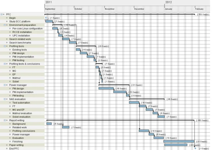
(11) Cross-layer power management for PGAS on SCC. Marc Gamell. domains of 8 cores. Finally, based on our observations, we provide a set of recommendations and insights that can be used to support similar power management for PGAS applications on other many-core platforms.. 1.4. Planning. Figure 1.1 shows the gantt diagram that represents the planning done at the beginning of the work. Jobs are distributed as described below: • The first unavoidable phase is needed to study how the experimental SCC platform works, and the basis of UPC Runtime. There is also a need to prepare the environment and search the existing related work. • A second phase is needed to approach application’s behavior. In order to achieve this target we need to look for several UPC benchmarks which can run on the constrained SCC environment, and profile its behavior. Therefore, we need to port existing profiling tools to SCC or prepare a lightweight instrumentation platform. • While extracting conclusions from the profiling phase, we can work on the power manager: a middleware which can take energy-efficiency related decisions. • Finally, we will need to evaluate the designed and implemented algorithm by executing a big set of tests. Note that, during the whole process (specially during periods in which the SCC is running tests), we will need to document the work, in order to avoid the final-term increased workload.. 1.5. Organization. The rest of this report is organized as follows. Chapter 2 presents the architecture of the SCC processor and specific SCC platform used in our experiment, with special focus on power management aspects that are important for our evaluation. Chapter 3 introduces PGAS parallel programming model and focus on one of its incarnations: UPC language. Chapter 4 discusses relevant related work. Chapter 5 contains a study of power behaviors of PGAS applications based on application profiling, with the goal of identifying opportunities for power management. Chapter 6 presents the proposed programming extensions and power management system for UPC PGAS applications on SCC, while chapter 7 presents their evaluation. Finally, chapter 8 concludes the report and outlines directions for future work.. 4.

(12) Cross-layer power management for PGAS on SCC. Figure 1.1: Planning: Gantt diagram.. 5. Marc Gamell.

(13) Chapter 2. Single-chip Cloud Computer background 2.1. Many-core motivation. In the recent years, as discussed by Borkar [5], processors has been shifted towards multi-core architectures: the idea is to include in a processor more simpler cores, than less complex ones. Note that the multi-core processor definition (a system with two or more independent processors packed together) can be applied to many-core systems too. We can find the main difference, however, in the number1 and complexity of these cores. While a multi-core processor have got several complex cores, a many-core processor have got a large number of cores that are much simpler than multi-core ones. Complex cores are faster, but simpler cores are smaller, in terms of die-area. If we apply Pollack’s Rule (performance increase is roughly proportional to square root of increase in complexity) inversely, performance of a smaller core reduces as square-root of the size, but power reduction is linear, resulting in smaller performance degradation with much larger power reduction. Overall, the compute throughput of the system, on the other hand, increases linearly with the larger number of small cores. That is why we can suppose that future processors will be based, in some way, in many-core processors.. 2.2. Intel SCC’s architecture overview. Intel Labs has created an experimental many-core processor, inside the Intel’s Tera-scale Computing Research Program, aimed to help accelerate many-core research and development. It is Single-chip Cloud Computer (SCC), and, as we can see in figure 2.1a, it consists of 48 x86 Pentium P54C cores, with increased L1 cache to 16 KB for data and another 16 KB for instructions and 256 KB of L2 cache per core. It is fabricated in a 45 nm process, and it’s cache is non-coherent: libraries like RCCE (studied below), however, offers software-based cache coherence implementation. It’s cores are grouped 2 by 2 in so-called tiles. 1 Usually,. many-core means 32 or more cores, while multi-core means fewer.. 6.

(14) Cross-layer power management for PGAS on SCC. (3,0). (3,5). (0,0). (0,5). (a) Architecture overview. Marc Gamell. (b) Packed chip. Figure 2.1: Single-chip Cloud Computer SCC features a fast (256 GB/s bisection bandwidth) 24-router on-die mesh network, with hardware support for message-passing, that communicates all tiles between them. This hardware message-passing support is helped by special per-tile 16 KB fast-r/w buffer, called message passing buffer (MPB). Therefore, every tile also includes a traffic generator (TG) used for ensure network reliability. Note that the on-chip network also provides tile access to four dual-channel DDR3 memory controllers (MC) with typically 32 GB or maximum 64 GB of main memory for the entire chip. The memory controllers are attached to the routers of the tiles at coordinates (0,0), (0,5), (2,0) and (2,5). As Single-chip Cloud Computer’s (SCC) name reflects, it implements an on-die scalable cluster of computers such as you would find in a cloud datacenter. The network topology and the message-passing implementation is proven to scale to thousands of processors in existing cloud datacenters. Moreover, each core can run a separate OS (typically Linux) and software stack and act like an individual compute node that communicates with other compute nodes over a packet-based network. SCC is intended to offer fine-grained power management, allowing to dynamically scale pertile frequency, and dynamically scale group-of-eight-core’s voltage. The power consumption can oscillate from 125 W to as low as 25W. This feature is what we are trying to exploit.. 2.3. Other existing many-cores. As mentioned in [16], SCC has been influenced by previous architectures and research. Beginning on the Cell processor, which wasn’t homogeneous and included 8 small SPE cores, SCC have been influenced by Polaris, a Intel 80-core experimental processor, which cores was simpler than x86’s SCC cores. On the other hand, there are other many-core architectures intended to be graphic proces7.

(15) Cross-layer power management for PGAS on SCC. Marc Gamell. sors. An example of this are the well known GPU architectures which must be programmed with special frameworks such as CUDA or OpenCL, as they are not x86. Another example is Intel’s Larrabee, which, like SCC, features x86 cores, with added support to vector processing.. 2.4. Memory. As mentioned above, SCC cores are regular x86 P54C cores. That means that it uses 32 bits to address the main memory. However, to access a main memory position we need to address one of four memory controllers, and a concrete position inside the 16 GB associated to that memory controller. As a result, we need 8 bits to point to the position of the MC in the mesh and 34 bits to address 16 GB. The difference between both addresses length is solved using a per-core lookup table (LUT), that translates a 32 bit core address to the corresponding system address. It is implemented as an area in the configuration block, and contains 256 22-bit positions. The 8 higher bits of a core address are used to point to a position of the LUT, which returns the 22 extra positions to fit the system address. This process is shown in figure 2.2, in which subdestination field points to a position inside a tile (i.e. core0, core1, MPB, east port, west port...) and a bit for MIU bypass. core address (32b) 8b. 1b. 8b. 3b. 24b. 10b. 24b. bypass dest subdest MC address. MC's memory address (34b). Figure 2.2: SCC LUT translation process. An SCC advantage is that LUT can be changed in run-time, meaning that we can redimension the core memory and/or the shared memory in order to adequate it to workload requirements. The cores of the SCC are grouped into four memory domains, depending on which memory controller (MC) holds the core main memory. As we have seen talking about LUT, this table determines which MC is responsible for which core. That is why memory domains are not fixed. However, the standard configuration is to assign each core to the nearest MC. This results on a vertical and horizontal division exactly in the middle of SCC, leaving 6 tiles per memory controller and a maximum hop number of 3 to reach the corresponding memory controller’s router.. 8.

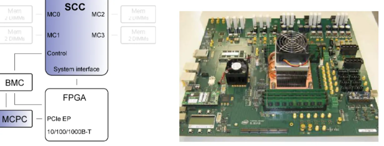
(16) Cross-layer power management for PGAS on SCC. 2.5. Marc Gamell. Mesh. Each tile is provisioned with a four-port router, in charge of the tile-to-tile connections, and with a Mesh Interface Unit (MIU), in charge of pack, unpack and address decode, among other related functions. These routers, the MIUs, and their corresponding connections forms the so-called mesh, a 6x4 two-dimensional squared grid that connects each tile with surrounding tiles and other entities like memory controllers, voltage regulator or system interface. This packet-switched network is governed by a simple deterministic (x,y) routing scheme. This means that data packets are routed first horizontally and finally vertically.. 2.6. SCC’s message passing library. SCC tools includes RCCE, a library that implements message passing functions specifically optimized to the SCC architecture. It takes profit of tile MPB’s and the fast mesh. The library also supports high level abstractions that handles voltage or frequency scaling operations or simplifies shared memory allocation.. 2.7. Rocky-Lake (SCC board) architecture. The experimental SCC chip needs a concrete environment to properly run, as it is not directly bootable. That is why a standard PC is used to control and manage SCC status, called management console PC (MCPC). The complete system’s architecture used for the work in this study (rocky lake board) is shown in figure 2.3a. As we can see, the SCC chip is connected directly to 8 memory dimms, totaling 32 GB. On the other hand, an ARM processor called Board Management Controller (BMC) is connected to the SCC and can handle commands like platform initialization or power data collecting. Furthermore, it is connected, via the system interface, to a FPGA that controls it’s external communications. Specifically, in addition to general purpose ports (22 I/O signals, SATA and PCIe interfaces) and a connection to the BMC, FPGA includes several ports (PCIe and Gigabit Ethernet) for connecting to the management PC.. 2.8. Power management capabilities. As mentioned above, RCCE provides tools that abstracts power management details in SCC. In this section, however, we are trying to explain which are SCC power management capabilities and which limitations have it got. Microprocessor’s power management can be done over the whole processor, or in specific areas (for example, cores). SCC, compared to existing processors, allows fine-grained power management. SCC have got three components that works with different clock and power source: mesh, memory controllers and tiles. On the one hand, the frequency of the entire mesh can operate from 800 MHz to 1.6 GHz. On the other hand, memory controllers operates from 800 to 1066 MHz. However, as soon as mesh and memory frequency and voltage changes cannot be performed during run-time, in this study we are focusing only on tile and voltage-domain power management.. 9.

(17) Cross-layer power management for PGAS on SCC. Marc Gamell. FPGA PCIe EP 10/100/1000B-T. (a) Rocky Lake System architecture. (b) Rocky Lake Board. Figure 2.3: Rocky Lake Board SCC cores are grouped 8 by 8 in six voltage domains, as shown in figure 2.4a, and voltage can only be changed in the scope of a whole voltage domain. Similarly, as shown in figure 2.4b, so-called frequency domains corresponds to tiles, and, therefore, frequency can only be changed tile by tile.. Single Chip Cloud. Single Chip Cloud. 39. 39. vDom 0. vDom 1. vDom 3. 27. 27. 33. 15. 15. vDom 4 0. 33. vDom 5. vDom 7 0. 6. (a) Voltage domains. 6. (b) Frequency domains. Figure 2.4: Domains in the SCC The part of the processor involved in the voltage is called the VRC (Voltage Regulator Controller), that works in a command-based strategy: cores sends messages with VRC destination, including the command. There is no limit in the source core of a command, which means that a core in a voltage domain can change the voltage of another domain, which can be very useful for sophisticated power management. The VRC is not distributed in every voltage domain, but it is a standalone part, reachable via the mesh by all cores. Therefore, the VRC only accepts one command at a time and, theoretically, the state is not defined if two cores sends respectively commands simultaneously. That is why a core can send a command three times in order to be sure the command have been finished. The first command will result in the actual change while the 10.

(18) Cross-layer power management for PGAS on SCC. Marc Gamell. last two ones would assure the change process have been finished. As described in [2], VRC allows voltage requests with a granularity of 6.25 mV, between 0 and 1.3 V. However, we found that the lower subrange of this voltages cannot be used in practice, as cores both crashes or become unstable. To remain safe, the lowest voltage used (with their corresponding lowest frequency) was 0.65625 V. We experimentally determined that this process takes an average of 40.2 ms to complete, regardless the originating-tile frequency or voltage and the desired voltage. Frequency scaling involved part, however, is distributed among tiles. Each tile contains a configuration register that is used to change the frequency divider, which can be any integer value between 2 and 16. As soon as global clock frequency is 1.6 GHz, resulting frequency oscillate between 800 to 100 MHz. When the process of writing the desired value in the register have been finished, the processor takes as little as 20 clock cycles to complete the actual frequency change. Before changing the voltage, however, the frequency must be changed accordingly to the desired voltage level. Similarly, when changing frequency we must take care the current voltage in the corresponding voltage domain. In the RCCE source code and in the SCC Programmers Guide there is a table showing the maximum frequency allowed for a voltage level (see table 2.1). As SCC cores maximum frequency is 800 MHz, the useful part of the table, however, are the voltage levels 0, 1 and 4. Experimentally we found that the first two voltage levels seems not to be safe, as many times the voltage domain became unstable, as described in [16]. The frequencies that worked, in our case, are shown in table 2.2. Voltage Level. Voltage (volts). Max freq. (MHz). 0 1 2 3 4 5 6. 0.7 0.8 0.9 1.0 1.1 1.2 1.3. 460 598 644 748 875 1024 1198. Table 2.1: SCCProgrammersGuide, version 0.75, Table 9: Voltage and Frequency values Voltage Level. Voltage. Max freq.(MHz). Tested freq. (MHz). 0 1 4. 0.75 0.85 1.1. 460 598 875. 400 533 800. Table 2.2: Safer Voltage and Frequency values, experimentally determined. To sum up, despite dynamic voltage scaling is difficult to exploit due to large voltage domains, its energy reduction is far better than frequency scaling which, unlike happens with voltage, a change in frequency only has a linear impact on the energy consumption. However, this technique is far faster than voltage scaling, and more flexible due to the smaller domain size, and, therefore, it can be applied in more variety of scenarios.. 11.

(19) Cross-layer power management for PGAS on SCC. 2.8.1. Marc Gamell. Power monitoring. SCC chip does not provides monitoring tools itself. In order to collect the measured voltage and current consumption we can send, from the management PC, a query command to the BMC (see figure 2.3a). Thanks to this features we can automatically collect the measured power consumption, obtaining a sampling frequency of about 6,5 measures per second. Figure 2.5 shows us the SCC’s consumed power, according to the workload and the technique used. Note that DVFS allows exponential power reduction regardless the workload, and DFS technique only allows linear power reduction. Note too that 400 MHz (which corresponds to lowest voltage allowed (0.75 V) is a good DVFS target in order to save energy, as lower levels provide only little-saving with huge frequency reduction. 100. Power (W). 80. DFS no load DVFS no load DFS load EP DVFS load EP. 60. 40. 20. 0 100. 200. 300. 400 500 Frequency (Mhz). 600. 700. 800. Figure 2.5: Consumed power by SCC according to the workload and the technique (DFS / DVFS). The data have been collected in the 15 possible frequencies available.. 12.

(20) Chapter 3. Unified Parallel C background 3.1. PGAS. In order to help the development stage of parallel and distributed applications, in the last few decades there have been a lot of research about parallel design languages and techniques. Partitioned global address space (PGAS) paradigm is a relatively new model that proposes a easy-of-use solution to the parallelization problem. It assumes a global, shared memory space that is logically partitioned among all threads and, therefore, each portion of the memory is local to one of the processors. As each thread is aware of which data is local, the application can improve performance by exploiting data locality. The performance, however, is not the only PGAS focus. Another important goal is to enhance user productivity significantly by abstract details like thread synchronization or implement implicitly the message passing. The PGAS model is the basis of Unified Parallel C (UPC), Co-array Fortran (CAF), Titanium, Chapel and X10.. 3.2. UPC overview. Unified Parallel C is an ISO C 99 extension that supports explicit parallelization and the PGAS model. It tries to get the best points of several previous C parallel extensions (like PCP, AC or Split-C), hence the name. It uses a Single Program Multiple Data (SPMD) model of computation in which the same code runs independently on different threads, in parallel. Apart from the private variables (which can only be seen inside the process), the user can define shared variables, usually vectors, which UPC distributes following a default pattern or a specified one. All threads can read or write a defined shared variable, but each memory position is physically assigned to one processor. In case the R/W operation is local, the UPC implementation should write it directly. If it is not local, however, the implementation is the responsible of mapping the operation to the corresponding R/W message and send it to the processor with affinity to that memory position. 13.

(21) Cross-layer power management for PGAS on SCC. Marc Gamell. Aside from the easy-of-use of PGAS paradigm, UPC offers a high level control over data distribution among cores. Furthermore, it extends the standard C pointers allowing it to point to an arbitrary position of the shared space, regardless it have local affinity or not. Shared space allows both static and dynamic memory allocations, as standard C does for the corresponding private addresses. Moreover, we should pay attention to the ability of incremental performance improvements that UPC paradigm offers. The programmer can begin by designing the application as plain sequential C code, converting it, later, to a simple shared-memory implementation, sharing some vectors. The programmer can then improve the performance by tuning data locality layout. Finally, for critical applications, the programmer can go deeply and tune it by making the memory management and one-sided communications explicit. The UPC extensions to C are as simple as an explicitly parallel execution model (global constants THREADS and MYTHREAD), shared variables and pointers (shared token), synchronization primitives (such as barrier or lock) and memory management primitives (such as bulk memory copy memget operation). As C is a well-known language inside the HPC user community (as for example scientists), the learning curve for UPC is easy to achieve.. 3.3. Berkeley UPC. In our study we have been using Berkeley UPC, which is an open-source UPC implementation. It is composed basically of: • The Berkeley UPC Translator. This module compiles the UPC source code to ANSIcompliant C code which can be linked with the abstract-machine described by the UPC Runtime. • The Berkeley UPC Runtime, which includes platform-independent job/thread control, shared memory access (put/get operations and bulk transfer operations), shared pointer manipulation and arithmetic, shared memory management, UPC barriers and UPC locks. • GASNET is the layer below UPC Runtime, which is a portable high-performance low-level networking layer and, among other things, is the responsible of implementing communication algorithms such as remote memory access. It runs over a wide variety of high-performance networks such as well-known MPI, Infiniband, Myrinet GM, Cray Gemini, or even UDP.. 14.

(22) Chapter 4. Related work Our work is mainly centered in three topics: layered power management, many-core power management and PGAS power management. In the following sections we are describing the existing and ongoing research on these three topics.. 4.1. Layered power management research. Existing and ongoing research in power efficiency and power management has addressed the problem at different levels such as processor and other subsystems level, runtime/OS level and application level. Processor level Since processors dominate the system power consumption in HPC systems [25], processor level power management is the most addressed aspect at server level. The most commonly used technique for CPU power management is Dynamic Voltage and Frequency Scaling (DVFS), which is a technique to reduce power dissipation by lowering processor clock speed and supply voltage [17,18]. Operating system level OS-level CPU power management involves controlling the sleep states or the C-states [28] and the P-states of the processor when the processor is idle [29] [30]. The Advanced Configuration and Power Interface (ACPI) specification provides the policies and mechanisms to control the C-states and P-states of the processor when they are idle [38]. Workload level Some of the most successful approaches for workload-level CPU power management were based on overlapping computation with communication in MPI programs, using historical data and heuristics [14, 15, 20, 22, 34], based on application profiles [6, 32], scheduling mechanisms [8] or exploiting low power modes when a task is not in the critical path [35]. Another result is that we can take profit of slack CPU periods slowing it down, and, therefore, saving energy. The problem have been to determine which periods are the appropriate. Here, the policies varies in complexity. Scheduled communication techniques take profit of the big difference between network and CPU speeds, and, while the application asks for a barrier, a synchronous send, or a synchronous receive and the processor is waiting for the transmission to finish, the runtime slow it down (by applying DVFS techniques) to save energy. Examples of this techniques. 15.

(23) Cross-layer power management for PGAS on SCC. Marc Gamell. can be found in work by Liu et al. [24] or work by Lim et al. [23]. Compiler level Another targeted layer for power management have been the compiler. Wu et al. [42] introduced a dynamic-compiler-driven control for energy efficiency. A dynamic compiler (HP Dynamo, IBM DAISY or Intel IA32EL) is a runtime software system that compiles, modifies or optimizes a program as it runs. Application level Aforementioned techniques are transparent to the application. This means that the programmer does not need to modify its application. However, existing work has also addressed power efficiency and power management at the application level. For example, Eon [39] is a coordination language for power-aware computing that enables developers to adapt their algorithms to different energy contexts. Overall, however, any of the existing research have been addressed the power management in a cross-layer approach.. 4.2. Many-core research. Power management Existing power management research has also addressed many-core systems. For example, Majzoub et al. [26] introduced a chip-design approach to voltage-island formation, for the energy optimization of many core architectures. Alonso et al. [3] proposed extending the power-aware techniques of Dense Linear Algebra algorithms to SCC. Performance improvements Other approaches have considered the SCC platform but mainly from the performance perspective. For example, Rotta [33] discussed how to efficiently design and implement the different strategies for message passing on SCC. Pankratius [31] introduced an application-level automatic performance tuning approach on the SCC. Urena et al. [40] implemented an MPI runtime optimized for the SCC message passing capabilities, RCKMPI. Clauss et al. [9,10] improved message passing performance on SCC by adding a non-blocking communication extension to RCCE library. Van Tol et al. [41] introduced an efficient memcpy implementation.. 4.3. PGAS research. Existing PGAS research has focused mainly on its performance and scalability. Salama et al. [36] proposed a potential improvement of collective operations in UPC. Dinan et al. [11] proposed an hybrid programming paradigm based upon MPI and UPC models that try to improve performance limitations. Chen et al. [19] compare the performance of benchmarks compiled with their own optimizations in BUPC with that of HP UPC compiler. Tarek et al. [12,13] benchmarks UPC and propose compiler optimizations. Kuchera et al. [21] study the UPC memory model and memory consistency issues. Existing PGAS research on many-core systems is not very large. Chapman et al. [7] implemented the X10 programming language on the Intel SCC (using RCCE library) and performed a comparative study versus MPI using different benchmark applications. Serres et al. [37] ported Berkeley UPC to Tilera’s many-core Tile64. 16.

(24) Cross-layer power management for PGAS on SCC. Marc Gamell. Overall, these approaches do not directly translate to PGAS applications on many-core processors and, to the best of our knowledge, power management in the PGAS framework has not been addressed yet.. 17.

(25) Chapter 5. Profiling of UPC applications In this chapter we are trying to show the behavior of some UPC applications suitable to work on SCC processor. We show an analysis of some applications from the UPC implementation of the NAS Parallel Benchmarks specification (FT, MG and EP kernels), a matmul-based synthetic imbalanced application and an application for edge detection (Sobel) from the UPC official test suite.. 5.1. Methodology. In order to profile the UPC applications we need to have got some instrumentation that tells us which UPC runtime operations an application uses. Existing profiling tools are designed to be executed in traditional clusters with big amounts of memory. If we use it in the SCC constrained environment, our profiling would be biased due to the overhead of the profile process. For this reason we decided to implement a low-footprint instrumentation system (that we called pmi, for Power Management Instrumentation), currently working on UPC, but extensible to other PGAS runtimes. Our design tries to minimize the runtime part, and do the main work as a post data processing. This is represented in the figure 5.1 flow. As seen, we achieve low overhead by writing lightweight intermediate files containing data in raw binary format. Then, the application parses the stored data (timestamps of the corresponding begin and end for each call) and, automatically, generates logfiles and relevant plots.. Data processing. Runtime UPC application. UPC runtime. Data collecting. Data extraction. Flow. Figure 5.1: Global architecture of the profiling platform.. 18. Graphics generation.

(26) Cross-layer power management for PGAS on SCC. 5.2. Marc Gamell. NAS Parallel Benchmarks. NPB are a well-known benchmark collection for parallel computing, standardized by the NASA Advanced Supercomputing. The suite comprises a set of kernels and pseudoapplications that reflect different kinds of relevant computation and communication patterns used by a wide range of applications. Each kernel can be configured with several different versions. These versions, called classes, does not differ in the problem nature, the difference is mainly in the size of the data. Apart from the MPI version of NPB, distributed and maintained by the NASA, there are several more implementations in different languages. One of these is NPB in UPC language, that have been developed and distributed by the George Washington University. Note that this distribution does not implement the whole set of tests, only a part. Kernels have been manually optimized through techniques that mature UPC compilers should handle in the future. Therefore, researchers can choose the level of optimization they wants to run. As mentioned above, the evaluated kernels are FT (Fast Fourier Transforms), EP (embarrassingly parallel cpu-intensive code) and MG (Multi Grid). We executed each benchmark on the whole SCC (involving all 48 available cores) because we want to stress the whole platform to obtain the most real potential of power management in many-core environments. BT and SP benchmarks, which require the number of processors be a perfect square, doesn’t use all the SCC platform potential. Other NAS benchmarks, like CG, that needs powers of two number of threads, does not stress the whole 48-core SCC platform neither. That is why we discarded these algorithms.. 19.

(27) Cross-layer power management for PGAS on SCC. 5.2.1. Marc Gamell. NAS FT kernel. FT is a kernel that calculates three 1D Fast Fourier Transforms, one for each dimension of a 3D partial differential equation. It is floating-point computation intensive and requires long range communications. We can run several versions of the same NPB kernel. For our experiments, we have been using FT class C, optimization O1, that is the largest problem that runs on the SCC platform and, therefore, it is the one that takes more time to finish. After instrumentation phase, we have collected data and processed it as mentioned in the section above, obtaining results in a set of graphics. The most representatives are shown here.. 25. 100. 10. 20. Length (s). Length (s). 1 15. 10. 0.1. 0.01 5. 0. 0.001. up. cr. up up up up up up up up up up c c c c c c c c c c glo r all r fre r wa r all ri lo r loc r pu r pu r ge r me ck tp t t e a it loc k ba sh psh psh mge l a lloc ka ar ar ar t llo l l e e o c d d d ed d c ou o ble uble va va l l. (a) Linear scale.. 0.0001. up. cr. up up up up up up up up up up c c c c c c c c c c glo r all r fre r wa r all ri lo r loc r pu r pu r ge r me tp t t e a it loc ck k ba sh psh psh mge l a lloc ka ar ar ar t llo l l e e o c d d d ed d c ou o ble uble va va l l. (b) Logarithmic scale.. Figure 5.2: Length of FT calls. If we take attention to figure 5.2a, we can see that it represents the length of each UPC call. Note that the candles shows the maximum, minimum and average duration (in seconds) of the corresponding call. As we can see in the mentioned figure (and the more detailed logarithmic version, figure 5.2b), FT uses only 11 UPC runtime operations, but only memget and wait seems to be long enough for being the focus of energy savings strategies. There have been 1056 memgets and 136 barriers per core, so we can analyze how many of these are short and how many are long. In figures 5.3a and 5.3c (and the corresponding figures 5.3b and 5.3d, in logarithmic scale) we analyze the number of calls per delay that FT performed for wait and memget, respectively. The figures corresponding wait, shows us that, apart from the 2500 calls of almost-null slack periods, there are lots of calls that needs 1-4 seconds, 6-7 seconds and more than 10 seconds to finish. memget, however, only uses operations of almost-zero and around 3 seconds delay. The main conclusion of these tests is that FT have a communication-bound profile.. 20.

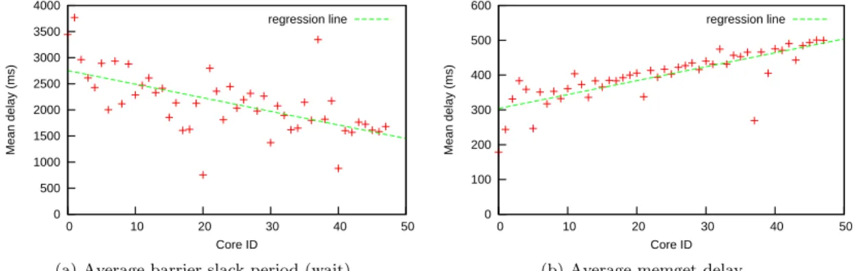
(28) Cross-layer power management for PGAS on SCC. Marc Gamell. 3000. 10000. 2500 1000 Number of calls. Number of calls. 2000. 1500. 100. 1000 10 500. 0. 1 0. 1000. 2000. 3000. 4000. 5000. 6000. 7000. 8000. 9000 >10000. 0. 1000. 2000. 3000. 4000. Length (ms). 5000. 6000. 7000. 8000. 9000 >10000. Length (ms). (a) Wait calls. Linear scale.. (b) Wait calls. Logarithmic scale.. 3500. 10000. 3000 1000 Number of calls. Number of calls. 2500. 2000. 1500. 1000. 100. 10. 500. 0. 1 0. 1000. 2000. 3000. 4000. 5000. 6000. 7000. 8000. 9000 >10000. 0. 1000. 2000. 3000. 4000. Length (ms). 5000. 6000. 7000. 8000. 9000 >10000. Length (ms). (c) Memget calls. Linear scale.. (d) Memget calls. Logarithmic scale.. Figure 5.3: Number of calls per delay.. 4000. 600 regression line. regression line. 3500. 500 Mean delay (ms). Mean delay (ms). 3000 2500 2000 1500. 400 300 200. 1000 100. 500 0. 0 0. 10. 20. 30. 40. 50. 0. 10. 20. Core ID. 30 Core ID. (a) Average barrier slack period (wait).. (b) Average memget delay.. Figure 5.4: Average delay of the call, per core.. 21. 40. 50.

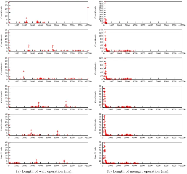
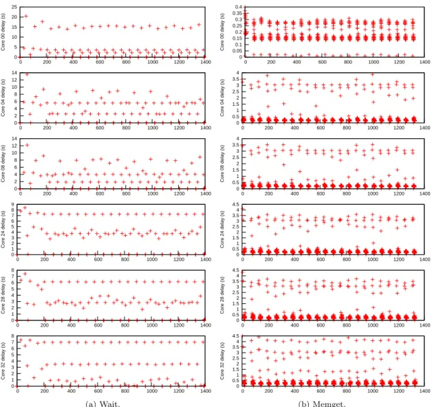
(29) Cross-layer power management for PGAS on SCC. Marc Gamell. 20 15 10. Core 00 calls. Core 00 calls. 30 25. 500 450 400 350 300 250 200 150 100 50 0. Core 04 calls. Note that in all these graphics we have been looking at the behavior of all cores together. In addition, the per-core behavior is notable. As we can see in figure 5.5a for waits, and figure 5.5b for memgets, each core have a different profile. Figure 5.6 shows the execution point in which each wait or memget call have been done, and their corresponding delays (in seconds). In these figures we can suspect that the average length is linearly dependent to the number of the core. If we look at the average of each call (figures 5.4a and 5.4b), per core, we will see that this suspect is not unfounded: there is a trend.. 140 120 100 80 60 40 20 0. 5 0. 0. Core 32 calls. 40 35 30 25 20 15 10 5 0. 3000. 4000. 4000. 5000. 5000. 6000. 6000. 7000. 7000. 8000. 8000. 9000. 9000. >10000. >10000. 0. 1000. 2000. 3000. 4000. 5000. 6000. 7000. 8000. 9000 >10000. 0. 1000. 2000. 3000. 4000. 5000. 6000. 7000. 8000. 9000 >10000. 0. 1000. 2000. 3000. 4000. 5000. 6000. 7000. 8000. 9000 >10000. Core 08 calls. 100 80 60 40 20 0. 0. 0. 0. 1000. 1000. 1000. 1000. 2000. 2000. 2000. 2000. 3000. 3000. 3000. 3000. 4000. 4000. 4000. 4000. 5000. 5000. 5000. 5000. 6000. 6000. 6000. 6000. 7000. 7000. 7000. 7000. 8000. 8000. 8000. 8000. 9000. 9000. 9000. 9000. >10000. Core 24 calls. Core 24 calls Core 28 calls. 40 35 30 25 20 15 10 5 0. 2000. 3000. 120. 0 35 30 25 20 15 10 5 0. 1000. 2000. 80 70 60 50 40 30 20 10 0. Core 28 calls. 35 30 25 20 15 10 5 0. 1000. 80 70 60 50 40 30 20 10 0. Core 32 calls. Core 04 calls Core 08 calls. 0 35 30 25 20 15 10 5 0. 80 70 60 50 40 30 20 10 0. >10000. >10000. >10000. (a) Length of wait operation (ms).. 0. 1000. 2000. 3000. 4000. 5000. 6000. 7000. 8000. 9000. >10000. 0. 1000. 2000. 3000. 4000. 5000. 6000. 7000. 8000. 9000. >10000. 0. 1000. 2000. 3000. 4000. 5000. 6000. 7000. 8000. 9000. >10000. (b) Length of memget operation (ms).. Figure 5.5: Number of operation calls per length (in ms). Each subplot represents a power domain controller.. 22.

(30) Core 00 delay (s). 5. Core 04 delay (s). 10. 4 3.5 3 2.5 2 1.5 1 0.5 0. Core 08 delay (s). 15. 0.4 0.35 0.3 0.25 0.2 0.15 0.1 0.05 0. 4 3.5 3 2.5 2 1.5 1 0.5 0. Core 24 delay (s). Core 00 delay (s). 25 20. 4.5 4 3.5 3 2.5 2 1.5 1 0.5 0. Core 28 delay (s). Marc Gamell. 4.5 4 3.5 3 2.5 2 1.5 1 0.5 0. Core 32 delay (s). Cross-layer power management for PGAS on SCC. 4.5 4 3.5 3 2.5 2 1.5 1 0.5 0. 0. Core 04 delay (s) Core 08 delay (s). 14 12 10 8 6 4 2 0. Core 24 delay (s). 9 8 7 6 5 4 3 2 1 0. Core 28 delay (s). 8 7 6 5 4 3 2 1 0. Core 32 delay (s). 0 14 12 10 8 6 4 2 0. 8 7 6 5 4 3 2 1 0. 0. 0. 0. 0. 0. 200. 200. 200. 200. 200. 200. 400. 400. 400. 400. 400. 400. 600. 600. 600. 600. 600. 600. 800. 800. 800. 800. 800. 800. 1000. 1000. 1000. 1000. 1000. 1000. 1200. 1200. 1200. 1200. 1200. 1200. 1400. 0. 1400. 1400. 1400. 1400. 1400. (a) Wait.. 200. 400. 600. 800. 1000. 1200. 1400. 0. 200. 400. 600. 800. 1000. 1200. 1400. 0. 200. 400. 600. 800. 1000. 1200. 1400. 0. 200. 400. 600. 800. 1000. 1200. 1400. 0. 200. 400. 600. 800. 1000. 1200. 1400. 0. 200. 400. 600. 800. 1000. 1200. 1400. (b) Memget.. Figure 5.6: Operation calls and corresponding delays (in seconds) according to execution point (in seconds). Each subplot represents a power domain controller. The conclusion of this part is that, although FT is well-balanced, some cores suffer from big slack periods. Therefore, FT can be a good candidate in order to study UPC power management techniques.. 23.

(31) Cross-layer power management for PGAS on SCC. 5.2.2. Marc Gamell. NAS MG kernel. MG, that stands for Multi Grid, is a benchmark that solves a 3D scalar Poisson equation. It performs both structured short and long range communications. In our profiling process we have been using MG class C, optimization O3, because it is the maximum that supports SCC constrains.. 30. 100. 25. 10. 20. 1 Length (s). Length (s). As we can see in figure 5.7, MG features mainly wait and two types of get_pshared calls.. 15. 0.1. 10. 0.01. 5. 0.001. 0. up. cr. up. up. cr. glo. ba. cr. wa. la. it. llo. c. up all. up up up up up up c c cr cr cr cr ge pu ge me loc r loc r pu tp tp tp tp k k sh sh sh sh mpu ka ar ar ar ar t llo e e e d d d d ed d c ou o ble uble va va l l. loc. cri. (a) Linear scale.. 0.0001. up. cr. up up up u up up up up up c c cri pcr c c c c c glo r wa r all loc r pu r ge r pu r ge r me l tp t t t it loc ock k ba sh psh psh psh mpu la ka ar ar ar ar t llo l l e e e o c d d d d ed d c ou o ble uble va va l l. (b) Logarithmic scale.. Figure 5.7: Length of MG calls. Let’s analyze first wait behavior. In figures 5.8a and 5.8b we can observe that MG performs lots of barriers (about 1200 per core), and, on average, the corresponding waits are short (about 5 to 30 ms). However, figure 5.8c shows that only a little quantity of calls are very long (10 seconds or more), while the bast majority are less than 0.25 seconds. Finally, with the help of figure 5.8d we can figure out this behavior: there is only one imbalanced barrier at the beginning of the execution (in the initialization phase), and the rest of the MG execution is well-balanced. The conclusions obtained from the wait analysis can be applied to get_pshared (figure 5.9): there are lots of small calls (25000 calls per core, 0.5 ms on average), and only one huge call, on the initialization phase. The same conclusions can be drawn for get_pshared_doubleval operation (see figure 5.10). With all this conclusions in mind, we see why MG does not show energy saving opportunities.. 24.

(32) Cross-layer power management for PGAS on SCC. Marc Gamell. 45. 1400 regression line. 40. 1200 1000. Number of calls. Mean delay (ms). 35 30 25 20 15. 800 600 400. 10 200. 5 0. 0 0. 10. 20. 30. 40. 50. 0. 5. 10. 15. 20. Core ID. 50. 20 15 10. 0. 0. 0. 1000. 1000. 1000. 1000. 2000. 2000. 2000. 2000. 2000. 3000. 3000. 3000. 3000. 3000. 4000. 4000. 4000. 4000. 4000. 5000. 5000. 5000. 5000. 5000. 6000. 6000. 6000. 6000. 6000. 7000. 7000. 7000. 7000. 7000. 8000. 5. 8000. 8000. 8000. 8000. 9000 >10000. Core 04 delay (s) 0. 1000. 16 14 12 10 8 6 4 2 0. Core 08 delay (s). Core 32 calls. 800 700 600 500 400 300 200 100 0. 45. 25. 16 14 12 10 8 6 4 2 0. Core 24 delay (s). Core 04 calls Core 08 calls Core 24 calls Core 28 calls. 800 700 600 500 400 300 200 100 0. 40. 0 0. 800 700 600 500 400 300 200 100 0. 35. 30 Core 00 delay (s). 800 700 600 500 400 300 200 100 0. 800 700 600 500 400 300 200 100 0. 30. (b) Total calls per core. 16 14 12 10 8 6 4 2 0. Core 28 delay (s). Core 00 calls. (a) Mean delay per core. 800 700 600 500 400 300 200 100 0. 25 Core ID. 8 7 6 5 4 3 2 1 0. 9000 >10000. 9000 >10000. 9000 >10000. 9000 >10000. 0. 50. 100. 150. 200. 250. 0. 50. 100. 150. 200. 250. 0. 50. 100. 150. 200. 250. 0. 50. 100. 150. 200. 250. 150. 200. 250. 0. 50. 100. Core 32 delay (s). 0.2 0.15 0.1 0.05 0 0. 1000. 2000. 3000. 4000. 5000. 6000. 7000. 8000. 9000 >10000. (c) Number of operation calls per length (in ms).. 0. 50. 100. 150. 200. 250. (d) Calls and corresponding delays (in seconds) according to execution point (in seconds).. Figure 5.8: MG wait behavior. 25.

(33) Cross-layer power management for PGAS on SCC. Marc Gamell. 0.8. 30000 regression line. 0.7. 25000 Number of calls. Mean delay (ms). 0.6 0.5 0.4 0.3. 20000 15000 10000. 0.2 5000. 0.1 0. 0 0. 10. 20. 30. 40. 50. 0. 5. 10. 15. 20. Core ID. (a) Mean delay per core. Core 00 delay (s). Core 00 calls. 25000 20000 15000 10000 5000 0 6000. 7000. 8000. 9000 >10000. 0. Core 04 calls. 30000 25000 20000 15000 10000 5000. Core 04 delay (s). 5000. 7 6 5 4 3 2 1 0. Core 08 delay (s). 4000. 7 6 5 4 3 2 1 0. Core 24 delay (s). 3000. 7 6 5 4 3 2 1 0. Core 28 delay (s). 2000. 7 6 5 4 3 2 1 0 7 6 5 4 3 2 1 0. 0 0. 1000. 2000. 3000. 4000. 5000. 6000. 7000. 8000. 9000 >10000. Core 08 calls. 30000 25000 20000 15000 10000 5000 0 0. 1000. 2000. 3000. 4000. 5000. 6000. 7000. 8000. 9000 >10000. Core 24 calls. 30000 25000 20000 15000 10000 5000 0 0. 1000. 2000. 3000. 4000. 5000. 6000. 7000. 8000. 9000 >10000. Core 28 calls. 30000 25000 20000 15000 10000 5000 0 0. 1000. 2000. 3000. 4000. 5000. 6000. 7000. 8000. 9000 >10000. Core 32 calls. 30000 25000 20000 15000 10000 5000 0 0. 1000. 2000. 3000. 4000. 5000. 35. 40. 45. 50. 6000. 7000. 8000. 0.08 0.07 0.06 0.05 0.04 0.03 0.02 0.01 0. Core 32 delay (s). 1000. 30. (b) Total calls per core. 30000. 0. 25 Core ID. 9000 >10000. (c) Number of operation calls per length (in ms).. 50. 100. 150. 200. 250. 0. 50. 100. 150. 200. 250. 0. 50. 100. 150. 200. 250. 0. 50. 100. 150. 200. 250. 0. 50. 100. 150. 200. 250. 0. 50. 100. 150. 200. 250. (d) Calls and corresponding delays (in seconds) according to execution point (in seconds).. Figure 5.9: MG get pshared behavior. 26.

(34) Cross-layer power management for PGAS on SCC. Marc Gamell. 200. 300 regression line. 180. 250. 140. Number of calls. Mean delay (ms). 160. 120 100 80 60. 200 150 100. 40. 50. 20 0. 0 0. 10. 20. 30. 40. 50. 0. 5. 10. 15. 20. Core ID. (a) Mean delay per core. Core 00 delay (s). Core 00 calls. 200 150 100 50. 50. 0.006 0.004 0.002. 0. 1000. 1000. 2000. 2000. 2000. 3000. 3000. 3000. 3000. 4000. 4000. 4000. 4000. 4000. 5000. 5000. 5000. 5000. 5000. 5000. 6000. 6000. 6000. 6000. 6000. 6000. 7000. 7000. 7000. 7000. 7000. 7000. 8000. 8000. 8000. 8000. 8000. 8000. 9000 >10000. 0. Core 04 delay (s) 0. 1000. 2000. 3000. 4000. 8 7 6 5 4 3 2 1 0. Core 08 delay (s) 0. 1000. 2000. 3000. 8 7 6 5 4 3 2 1 0. Core 24 delay (s). 0. 1000. 2000. 8 7 6 5 4 3 2 1 0. Core 28 delay (s). 0. 1000. 8 7 6 5 4 3 2 1 0. Core 32 delay (s). Core 04 calls Core 08 calls Core 24 calls Core 28 calls Core 32 calls. 140 120 100 80 60 40 20 0. 45. 0 0. 140 120 100 80 60 40 20 0. 40. 0.008. 0. 140 120 100 80 60 40 20 0. 35. 0.01. 250. 140 120 100 80 60 40 20 0. 30. (b) Total calls per core. 300. 140 120 100 80 60 40 20 0. 25 Core ID. 8 7 6 5 4 3 2 1 0. 9000 >10000. 9000 >10000. 9000 >10000. 9000 >10000. 9000 >10000. (c) Number of operation calls per length (in ms).. 50. 100. 150. 200. 250. 0. 50. 100. 150. 200. 250. 0. 50. 100. 150. 200. 250. 0. 50. 100. 150. 200. 250. 0. 50. 100. 150. 200. 250. 0. 50. 100. 150. 200. 250. (d) Calls and corresponding delays (in seconds) according to execution point (in seconds).. Figure 5.10: MG get pshared doubleval behavior. 27.

(35) Cross-layer power management for PGAS on SCC. 5.2.3. Marc Gamell. NAS EP kernel. EP, the last NAS benchmark that we will use, is an embarrassingly parallel application that performs floating point operations with almost no-communication. In our study we have been running EP class D, without optimization, because it is the maximum configuration that supports SCC constrains. Beginning with figure 5.11, we can see that the long operations that EP uses are wait, upcr_lock, upcri_lock and get_pshared_doubleval. Note that both lock operations are equivalent, because one always calls the other in UPC Runtime implementation.. 70. 100. 60. 10. 50. Length (s). Length (s). 1 40. 30. 0.1. 0.01 20 0.001. 10. 0. up. cr. up. cr. glo. ba. up. cr. wa. la. it. llo. c. up all. cri. loc. up. cr. loc. ka. k. up. cr. loc. k. llo. c. up tp. sh. 0.0001. up. cr. pu. cr. pu. ar. tp. ed. sh. tp. ar. ed. up. cr. ge. sh. cr. ba. ed. ub. do. up. cr. wa. it. la. ar. do. up glo. llo. c. up all. cri. loc. up. cr. loc. k. ka. up. cr. loc. k. up. llo. c. ub. lev. al. cr. pu. tp. sh. up. cr. pu. ar. tp. ed. sh. ge. tp. ar. ed. sh. ar. do. ed. ub. lev. al. (a) Linear scale.. do. ub. lev. al. lev. (b) Logarithmic scale.. Figure 5.11: Length of EP calls. As in the previous analysis, we begin studying wait operation profile on EP kernel. The first conclusion drawn from figure 5.12 is that there are only 9 calls per core and 8 have got insignificant delays. The ninth one corresponds to the barrier at the end of execution, and is large (18 seconds) because it accumulates the short imbalance through all the execution. In figure 5.13b we can observe that there is only one lock call in the whole execution. This makes lock a bad candidate for energy savings opportunities. Finally, as we can see in the set of figures 5.14, get_pshared_doubleval operation, that initially seemed interesting, is not interesting from energy savings point of view, because there are only few and short calls in 47 cores, and only in the first core the delay is, sometimes, large. Although common sense tells us that CPU-intensive applications are not suitable for energy savings, this study shows us that EP does not give many energy savings opportunities, because EP’s profile is not communication-bound nor memory-bound.. 28. al.

(36) Cross-layer power management for PGAS on SCC. Marc Gamell. 2000. 9 regression line. 1800. 8 7. 1400. Number of calls. Mean delay (ms). 1600. 1200 1000 800 600. 6 5 4 3. 400. 2. 200. 1. 0. 0 0. 10. 20. 30. 40. 50. 0. 5. 10. 15. Core ID. 8000. Core 00 calls. Core 00 delay (s) 7000. Core 04 delay (s). 6000. 18 16 14 12 10 8 6 4 2 0. Core 08 delay (s). 5000. 18 16 14 12 10 8 6 4 2 0. Core 24 delay (s). 4000. 18 16 14 12 10 8 6 4 2 0. Core 28 delay (s). 3000. 18 16 14 12 10 8 6 4 2 0. 18 16 14 12 10 8 6 4 2 0. Core 32 delay (s). 2000. 18 16 14 12 10 8 6 4 2 0. 9000 >10000. Core 04 calls. 4 3.5 3 2.5 2 1.5 1 0. 1000. 2000. 3000. 4000. 5000. 6000. 7000. 8000. 9000 >10000. Core 08 calls. 4 3.5 3 2.5 2 1.5 1 0. 1000. 2000. 3000. 4000. 5000. 6000. 7000. 8000. 9000 >10000. Core 24 calls. 4 3.5 3 2.5 2 1.5 1 0. 1000. 2000. 3000. 4000. 5000. 6000. 7000. 8000. 9000 >10000. Core 28 calls. 4 3.5 3 2.5 2 1.5 1. Core 32 calls. 0. 1000. 2000. 3000. 4000. 5000. 6000. 7000. 8000. 9000 >10000. 5 4.5 4 3.5 3 2.5 2 1.5 1 0. 1000. 2000. 3000. 4000. 5000. 6000. 30. 35. 40. 45. 50. (b) Total calls per core. 5 4.5 4 3.5 3 2.5 2 1.5 1 1000. 25 Core ID. (a) Mean delay per core. 0. 20. 7000. 8000. 9000 >10000. (c) Number of operation calls per length (in ms).. 0. 200. 400. 600. 800. 1000. 1200. 1400. 0. 200. 400. 600. 800. 1000. 1200. 1400. 0. 200. 400. 600. 800. 1000. 1200. 1400. 0. 200. 400. 600. 800. 1000. 1200. 1400. 0. 200. 400. 600. 800. 1000. 1200. 1400. 0. 200. 400. 600. 800. 1000. 1200. 1400. (d) Calls and corresponding delays (in seconds) according to execution point (in seconds).. Figure 5.12: EP wait behavior. 29.

(37) Cross-layer power management for PGAS on SCC. Marc Gamell. 70000. 1 regression line. 60000 Number of calls. Mean delay (ms). 0.8 50000 40000 30000 20000. 0.6. 0.4. 0.2 10000 0. 0 0. 10. 20. 30. 40. 50. 0. 5. 10. 15. Core ID. Core 00 delay (s) Core 04 delay (s). 6.46 6.44 6.42 6.4 6.38 6.36 6.34 6.32 6.3. Core 08 delay (s). 20.2 20.15 20.1 20.05 20 19.95 19.9 19.85 19.8 19.75. Core 24 delay (s). 61 60.8 60.6 60.4 60.2 60 59.8 59.6. Core 28 delay (s). 1 0.995. 0.0101 0.01008 0.01006 0.01004 0.01002 0.01 0.00998 0.00996 0.00994 0.00992 0.0099. 7.32 7.3 7.28 7.26 7.24 7.22 7.2 7.18 7.16. Core 32 delay (s). Core 00 calls. 1.01. 16.2 16.15 16.1 16.05 16 15.95 15.9 15.85 15.8. 0.99 2000. 3000. 4000. 5000. 6000. 7000. 8000. 9000 >10000. -1. Core 04 calls. 1.01 1.005 1 0.995 0.99 0. 1000. 2000. 3000. 4000. 5000. 6000. 7000. 8000. 9000 >10000. -1. Core 08 calls. 1.01 1.005 1 0.995 0.99 0. 1000. 2000. 3000. 4000. 5000. 6000. 7000. 8000. 9000 >10000. -1. Core 24 calls. 1.01 1.005 1 0.995 0.99 0. 1000. 2000. 3000. 4000. 5000. 6000. 7000. 8000. 9000 >10000. Core 28 calls. 1.01 1.005 1 0.995 0.99 0. 1000. 2000. 3000. 4000. 5000. 6000. 7000. 8000. 9000 >10000. Core 32 calls. 1.01 1.005 1 0.995 0.99 0. 1000. 2000. 3000. 4000. 5000. 6000. 30. 35. 40. 45. 50. (b) Total calls per core. 1.005. 1000. 25 Core ID. (a) Mean delay per core. 0. 20. 7000. 8000. 9000 >10000. (c) Number of operation calls per length (in ms).. -0.5. -0.5. -0.5. 0. 0. 0. 0.5. 1. 0.5. 1. 0.5. 1. -1. -0.5. 0. 0.5. 1. -1. -0.5. 0. 0.5. 1. 0.5. 1. -1. -0.5. 0. (d) Calls and corresponding delays (in seconds) according to execution point (in seconds).. Figure 5.13: EP lock behavior. 30.

(38) Cross-layer power management for PGAS on SCC. Marc Gamell. 300. 300 regression line 250 Number of calls. Mean delay (ms). 250 200 150 100. 200 150 100. 50. 50. 0. 0 0. 10. 20. 30. 40. 50. 0. 5. 10. 15. 20. Core ID. (a) Mean delay per core. Core 00 delay (s). Core 00 calls. 200 150 100 50 0 1000. 2000. 3000. 4000. 5000. 6000. 7000. 8000. 9000 >10000. Core 04 delay (s). Core 04 calls. 12.1 12.05 12 11.95 11.9 1000. 2000. 3000. 4000. 5000. 6000. 7000. 8000. 50. 10. 20. 30. 40. 50. 60. 70. 80. 90. 0.5 0 -0.5. 9000 >10000. 0. 0.002. 0.004. 0.006. 0.008. 0.01. 0.008. 0.01. 0.008. 0.01. 0.01 Core 08 delay (s). Core 08 calls. 45. -1 0. 12 10 8 6 4 2. 0.008 0.006 0.004 0.002. 0. 0 0. 1000. 2000. 3000. 4000. 5000. 6000. 7000. 8000. 9000. >10000. 0. 0.002. 0.004. 0.006. 1 Core 24 delay (s). 12.15 Core 24 calls. 40. 1. 11.85. 12.1 12.05 12 11.95 11.9 11.85. 0.5 0 -0.5 -1. 0. 1000. 2000. 3000. 4000. 5000. 6000. 7000. 8000. 9000 >10000. 0. 0.002. 0.004. 0.006. 0.01 Core 28 delay (s). 12 Core 28 calls. 35. 35 30 25 20 15 10 5 0 0. 12.15. 10 8 6 4 2 0. 0.008 0.006 0.004 0.002 0. 0. 1000. 2000. 3000. 4000. 5000. 6000. 7000. 8000. 9000. >10000. 0. 0.002. 0.004. 0.006. 0.008. 0.01. 0. 0.002. 0.004. 0.006. 0.008. 0.01. 0.01 Core 32 delay (s). 12 Core 32 calls. 30. (b) Total calls per core. 250. 0. 25 Core ID. 10 8 6 4 2 0. 0.008 0.006 0.004 0.002 0. 0. 1000. 2000. 3000. 4000. 5000. 6000. 7000. 8000. 9000. (c) Number of operation calls per length (in ms).. >10000. (d) Calls and corresponding delays (in seconds) according to execution point (in seconds).. Figure 5.14: EP get pshared doubleval behavior. 31.

(39) Cross-layer power management for PGAS on SCC. 5.3. Marc Gamell. Sobel. Sobel is an edge detection application, a kind of applications useful in several fields such as computer vision. The parallelized version of this algorithm partitions the image among the cores, performs calculations locally and, when it needs to shift the data through the last row of a thread data, it access to the elements of the next row (allocated in the next contiguous core). The first step to analyze the Sobel application is to determine which UPC Runtime operations it uses. In figure 5.15 we can see that it uses wait and global_alloc. Note that during the instrumentation phase we disabled the upcr_get_pshared operation logging, because we observed that each core called it about 90 millions of times (89786623 calls); this huge amount of calls produced the execution time during instrumentation increase a lot, and that is why we decided to disable it to run the execution more realistic. 500. 100. 450 10 400 350 1 Length (s). Length (s). 300 250. 0.1. 200 0.01 150 100 0.001 50 0. up. cr. 0.0001. up. cr. glo. ba. up. cr. wa. la. it. up. cr. glo. ba. llo. c. (a) Linear scale.. wa. it. la. llo. c. (b) Logarithmic scale.. Figure 5.15: Length of Sobel calls. Like NAS benchmarks studied above, the next step is to observe the behavior of the main calls; in this case, only wait. We don’t show the results of upcr_get_pshared because all the calls are negligible. As we observe in figure 5.16, we should distinguish the behavior of the core 0 and the rest of the cores. One reason for this is due to the initialization phase, made only by core 0. Note that there is a barrier in the beginning of the execution, that delays the non-0 cores about 500 seconds, and this barrier is finished only when core 0 finishes the init phase and calls the corresponding barrier operation (see the lonely 0-delay point around position x = 480, in figure 5.16d). Once the initialization is done, the benchmark repeats N = 100 times the Sobel algorithm, synchronizing with a barrier at the end of each iteration. As we can see in figure 5.16c, the slack period corresponding to the wait operation is about 0.5 seconds on all cores except cores 0 and 47 (core 47 log is not shown in the figure because of a space matter), which are about 2 seconds long. Although this application does not seems very interesting from the point of view of the iterations phase (due to little imbalance), it can be useful to study the core-0 driven initialization phase. 32.

(40) Cross-layer power management for PGAS on SCC. Marc Gamell. 7000. 120 regression line 100. 5000. Number of calls. Mean delay (ms). 6000. 4000 3000 2000. 80 60 40 20. 1000 0. 0 0. 10. 20. 30. 40. 50. 0. 5. 10. 15. Core ID. Core 00 delay (s) Core 04 delay (s). 500 450 400 350 300 250 200 150 100 50 0. Core 08 delay (s). 5. 500 450 400 350 300 250 200 150 100 50 0. Core 24 delay (s). 10. 500 450 400 350 300 250 200 150 100 50 0. Core 28 delay (s). 15. 1.8 1.6 1.4 1.2 1 0.8 0.6 0.4 0.2 0. 500 450 400 350 300 250 200 150 100 50 0. Core 32 delay (s). Core 00 calls. 20. 500 450 400 350 300 250 200 150 100 50 0. 0 2000. 3000. 4000. 5000. 6000. 7000. 8000. 9000. >10000. Core 04 calls. 30 25 20 15 10 5 0 0. 1000. 2000. 3000. 4000. 5000. 6000. 7000. 8000. 9000. >10000. Core 08 calls. 25 20 15 10 5 0. Core 24 calls Core 28 calls. 0 14 12 10 8 6 4 2 0 20 18 16 14 12 10 8 6 4 2 0. 0. 0. 1000. 1000. 1000. 2000. 2000. 2000. 3000. 3000. 3000. 4000. 4000. 4000. 5000. 5000. 5000. 6000. 6000. 6000. 7000. 7000. 7000. 8000. 8000. 8000. 9000. 9000. 9000. >10000. >10000. >10000. Core 32 calls. 25 20 15 10 5 0 0. 1000. 2000. 3000. 4000. 5000. 6000. 30. 35. 40. 45. 50. (b) Total calls per core. 25. 1000. 25 Core ID. (a) Mean delay per core. 0. 20. 7000. 8000. 9000. (c) Number of operation calls per length (in ms).. >10000. 0. 100. 200. 300. 400. 500. 600. 700. 800. 900. 0. 100. 200. 300. 400. 500. 600. 700. 800. 900. 0. 100. 200. 300. 400. 500. 600. 700. 800. 900. 0. 100. 200. 300. 400. 500. 600. 700. 800. 900. 0. 100. 200. 300. 400. 500. 600. 700. 800. 900. 0. 100. 200. 300. 400. 500. 600. 700. 800. 900. (d) Calls and corresponding delays (in seconds) according to execution point (in seconds).. Figure 5.16: Sobel wait behavior. 33.

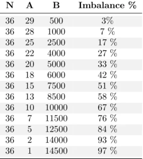
(41) Cross-layer power management for PGAS on SCC. 5.4. Marc Gamell. Matmul-based synthetic imbalanced application. In the profile of the UPC version of the NAS applications we have seen that wait is an usual operation. We know that this UPC Runtime instruction is used to implement barriers. That’s why we can suppose that the more imbalanced an application is, the more energy savings we will achieve. A parallel or distributed application is balanced if the slack period during a barrier is almost null. It is imbalanced if there are threads that spend lots of time waiting, in barriers (big slack periods), compared to other threads, which slack periods are almost null. The main goal of using the synthetic matmul is to study the potential of voltage scaling for different levels of load imbalance caused by barriers (wait operation).. 5.4.1. Algorithm. Basically, the main algorithm is: for (i=0 ; i<N ; i++) { perform A matrix multiplications, distributed in 48 cores; if(MYTHREAD is in Voltage Domain X) perform B matrix multiplications; upc_barrier; }. 5.4.2. Parameters. The parameters to control the behavior of the aforementioned algorithm are: N The number of overall iterations A The number of all 6 voltage domain distributed matrix multiplications B The number of only one voltage domain matrix multiplications The first set of tests performed with this benchmark was the regular execution (i.e. no power management), called in this document original tests or base tests. The parameters used in this set of tests are shown in the table 5.1, which relates the level of imbalanced produced by the parameters, and that is calculated experimentally, with the data collected during the execution. Another significant results from the collected data are the execution time, that was about 20 minutes per test and the consumed energy, about 105 KJ.. 34.

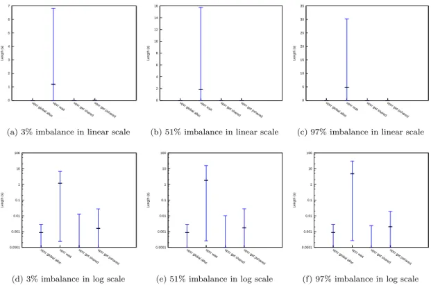
(42) Cross-layer power management for PGAS on SCC. Marc Gamell. N. A. B. Imbalance %. 36 36 36 36 36 36 36 36 36 36 36 36 36. 29 28 25 22 20 18 15 13 10 7 5 2 1. 500 1000 2500 4000 5000 6000 7500 8500 10000 11500 12500 14000 14500. 3% 7% 17 % 27 % 33 % 42 % 51 % 58 % 67 % 76 % 84 % 93 % 97 %. Table 5.1: Parameters used in the matmul original (or base) test.. 5.4.3. Conclusions. We ran matmul with load imbalances ranging from 3% to 97%. Figure 5.17 shows that wait calls are the largest ones (i.e. most energy-savings capable). The histograms and the mean delay per core plots of the wait calls are shown by figures 5.18 and 5.19, respectively. Note that in tests with very imbalanced applications (Figures 5.18b, 5.18e,5.18c and 5.18f) many calls are longer than 10 seconds. Comparing parameter B in table 5.1 and resulting wait calls in figure 5.20, we can see that the number of calls is directly proportional to the B parameter. Figure 5.21 shows the histogram of the wait operation length, while figure 5.22 shows the execution point in which each wait call have been done, and their corresponding delays (in seconds). The results show very different behaviors depending of the percentage of load imbalance. Specifically, longer wait calls correspond to larger load imbalance percentages.. 35.