Outflow of Weddell sea waters into the Scotia Sea through the western sector of the South Scotia Ridge

Texto completo

(1)OUTFLOW OF WEDDELL SEA WATERS INTO THE SCOTIA SEA THROUGH THE WESTERN SECTOR OF THE SOUTH SCOTIA RIDGE. A thesis submitted to the Department of Physics of the Universitat de les Illes Balears for the degree of Doctor of Physics by. Margarita Palmer García. Palma de Mallorca, November 2012.

(2)

(3) __________________________________________________________ Damià Gomis Bosch, Catedràtic d’Universitat del Departament de Física de la Universitat de les Illes Balears, CERTIFICA Que aquesta tesi ha estat realitzada per la Sra. Margarita Palmer García sota la seva direcció. I per a que així consti, firma la present, a Palma, a dia 5 de novembre de 2012. Damià Gomis Bosch __________________________________________________________.

(4)

(5) To my parents.

(6)

(7) ACKNOWLEDGEMENTS Looking backwards at the end of this research work, I remember that my first step in this field was an optional course offered as part of my degree in Physics. The topic was Physical Oceanography, and it was given, coincidences of life, by who some years later became the director of this PhD thesis, Dr. Damià Gomis. During the same period I also attended an optional course on Marine Biology (this one belonging to the degree in Biology), and I was fascinated by the pictures of the chapter devoted to Antarctica. I remember that after one of the lessons I went to a tutorial because there was something I couldn’t understand properly: it was related to the inshore currents around Antarctica and now I know that my question did not have an easy answer... But it was not until I applied for a PhD grant of the Spanish Ministry of Science and Innovation that I got deeply in contact with the world of Oceanography. Hence, first of all I have to thank Drs. Damià Gomis and M. Mar Flexas for giving me the opportunity of being part of this project (ESASSI, POL2006-11139-C02-01/CGL) and for their guidance and help during the development of this thesis. I also thank a contract from the Universitat de les Illes Balears that has covered the last period of this work. My implication in this project began in the best possible way: taking part in a cruise to the Southern Ocean. The ESASSI-08 cruise was actually the first cruise of my life, and it was to a region that few people have the opportunity to visit. I want to thank the scientists, technicians, officers and crew of R/V Hespérides for their contribution to the success of the cruise. I also want to thank all the people that have helped me in different aspects of this Thesis. In particular, Dr. Gabriel Jordà, for his introduction to the world of Matlab programming and for the pre-processing and de-tiding of ADCP data. Drs. Alberto C. Naveira-Garabato,. Loic. Jullion,. and. Takamasa. Tsubouchi. from. the. National. Oceanography Centre in Southampton for helping me with the inverse modeling and with the interpretation of results. Dr. T. Tsubouchi also helped me with the Optimum Multiparameter technique. I also want to thank Dr. Marta Álvarez for providing oxygen and nutrient data, Dr. Laurie Padman for providing the output of a new tidal model in the study region, Dr. Andrew F. Thompson for providing historical and ADELIE drifter observations and Dr. Josep M. Gili for his comments on the nutrient distribution in the Weddell-Scotia Confluence..

(8) Last, but not least, I am especially grateful to my family for their support and to my colleagues at IMEDEA for their friendship along these years..

(9) ABSTRACT This work compiles the results of the analysis of hydrographical data collected in January 2008 over the western sector of the South Scotia Ridge (SSR). The cruise was carried out on board R/V Hespérides in the framework of the Synoptic Antarctic Shelf-Slope Interaction (SASSI) study, one of the core projects endorsed by the International Polar Year. SASSI focused on shelf-slope processes taking place all along the Antarctic continental slope, paying particular attention to the Antarctic Slope Front (ASF) and its associated westward Antarctic Slope Current (ASC). The Spanish contribution to SASSI (framed by the E-SASSI project) focused on the SSR region between the South Shetland Islands and the South Orkney Islands, bounded to the north by the Scotia Sea and to the south by the Weddell Sea. The main objectives of E-SASSI were (1) to quantify the outflow of Weddell Sea waters into the Scotia Sea and to determine how these waters contribute to the modification of the Southern Boundary (SB) of the Antarctic Circumpolar Current (ACC); (2) to determine the role of the Antarctic Slope Front in these processes; and (3) to track the path of the Antarctic Slope Current before diluting into the Scotia Sea. This thesis aims to answer these questions. The sector of the SSR located between the South Shetland Islands and the South Orkney Islands is a region of especial interest. First because the gaps indenting the ridge constitute the first gate for the outflow of relatively shallow, recently ventilated waters from the northwestern Weddell Sea into the Scotia Sea. Second, because of the complexity of the bathymetry: a deep trough (the Hesperides Trough) separates the northern and southern flanks of the ridge and the location and depth of the different gaps indenting the ridge constrain the pathway of the Antarctic Slope Current. A key feature of the E-SASSI cruise with respect to previous studies conducted in the region is the unprecedented high spatial resolution of the hydrographic survey, particularly over the continental slopes. Also the coverage of all the gaps of the northern flank of the ridge was a novelty of E-SASSI. Both features have allowed a better quantification of the water mass transports in the region. The E-SASSI physical data consist mainly of Conductivity-Temperature-Depth (CTD) and ship-mounted Acoustic Doppler Currentmeter Profiler (ADCP) measurements. The presence of narrow jets, the rough topography, the strong tidal currents observed in the.

(10) region, and the fact that velocity measurements were available only for the upper 500 meters of the water column, they all handicapped the determination of the barotropic component of the flow. Inverse modeling based on the conservation of volume, heat, and salt over an enclosed region was used to refine the barotropic component of the velocity pattern initially estimated from the adjustment of the baroclinic component of velocity profiles to the ADCP measurements. The regional circulation, including the pathway of the Antarctic Slope Current, was inferred from the joint analysis of CTD profiles and the velocity field inferred from the inverse model. Results from a cross-slope section located in the Weddell Sea side show the well-defined structure of the Antarctic Slope Front before reaching the SSR. At the firsts gaps indenting the southern flank of the SSR the ASC has been observed to break into two branches: an inshore branch following the upper levels of the slope (700m) and an offshore branch extending over the 1600m isobath. At the northern flank the sampling covered all the gaps of the ridge and several cross-slope sections into the Scotia Sea. The inshore branch of the ASC was detected crossing a relatively shallow gap that prevents the outflow of the offshore, deeper branch and acts as a barrier for Weddell Sea Deep Water (WSDW). In spite of the higher velocities of the outflow, this shallow gap is less important in terms of Warm Deep Water (WDW) transport than the deeper Hesperides Passage hosting the outflow of the deeper branch of the ASC. This passage accounts for most of the outflow of Weddell Sea waters into the Scotia Sea and is the only gate of WSDW through the western sector of the SSR. The transports inferred from the inverse model give a net outflow of 7 ± 5 Sv, 2 Sv corresponding to WSDW and most of the other 5 Sv being WDW. In addition to the determination of the circulation pattern we have also analyzed inflow/outflow θS diagrams. They show an overall homogenization of the outflowing waters with respect to the more variable incoming Weddell Sea waters. In the last part of this thesis we show that isopycnal mixing between inshore and offshore water masses taking place within the Hesperides Trough is the main process for the modification of subsurface and intermediate layers. We also describe the role of the ASF in the formation of the most modified WDW observed before reaching the SSR and study the contribution of this water to the modification of the Southern Boundary of the ACC, in the southwestern sector of the Scotia Sea..

(11) RESUM Aquest treball reuneix els resultats de l’anàlisi de dades hidrogràfiques preses el gener de 2008 durant una campanya oceanogràfica a la Dorsal d’Escòcia del Sud (Antàrtida). La campanya es va dur a terme a bord del R/V Hespérides en el marc del projecte SASSI (Synoptic Antarctic Shelf-Slope Interaction study), un dels projectes clau de l’Any Polar International. Aquest projecte va tenir com a objectiu l’estudi de processos entre la plataforma i el talús continental antàrtics, amb una especial atenció al Front de Talús Antártic i al seu corrent associat que flueix en sentit oest, el Corrent de Talús Antàrtic. La contribució espanyola a SASSI (el projecte E-SASSI) es va centrar en el sector oest de la Dorsal d’Escòcia del Sud, entre les illes Shetland del Sud i Orcades del Sud, flanquejat al nord pel Mar d’Escòcia i al sud pel Mar de Weddell. Els objectius principals d’E-SASSI eren: (1) quantificar l’exportació d’aigües del Mar de Weddell cap al Mar d’Escòcia i determinar com aquestes aigües contribueixen a la modificació de la Frontera Sud del Corrent Circumpolar Antàrtic; (2) determinar el paper que juga el Front de Talús en tots aquests processos; i (3) traçar el camí que recorr el Corrent de Talús abans de diluir-se en el Mar d’Escòcia. Aquesta tesi tracta de respondre totes aquestes qüestions. El sector oest de la dorsal és d’especial interés. Primer perquè els passos que s’obren al llarg de la dorsal constitueixen la primera porta de sortida cap al Mar d’Escòcia d’aigües relativament poc fondes i recentment ventilades que flueixen al llarg del marge nordoest del Mar de Weddell. Segon, degut a la complexitat de la batimetria: la localització i fondària d’aquests passos, a més de l’existència d’una fossa submarina que separa aquesta banda de la dorsal en un flanc nord i un flanc sud (la Fossa d’Hespèrides), són tots factors que afecten al pas del Corrent de Talús per sobre de la dorsal. Els punts claus de la campanya E-SASSI respecte d’estudis precedents duïts a terme en aquesta regió són, d’una banda, l’elevada resolució espacial del mostreig hidrogràfic, sobretot al talús continental, i d’altra, la cobertura del mostreig, que abastà tots els passos del flanc nord de la dorsal. Ambdós aspectes han estat una aportació fonamental per part d’E-SASSI, per quan han permès una millor quantificació dels transports d’aigües en aquesta regió. El conjunt de dades físiques d’E-SASSI són majoritàriament dades de conductivitat, temperatura i pressió (Conductivity-Temperature-Depth, CTD) i de velocitat (Acoustic.

(12) Doppler Currentmeter Profiler, ADCP). La presència de corrents prims, lo abrupt de la batimetria, els forts corrents de marea observats a la regió, i el fet de disposar de mesures directes de la velocitat només en els primers 500 metres de la columna d’aigua, tot plegat fa que la determinació del component baròtrop del fluxe sigui complicada. La modelització inversa és una tècnica que es basa en la conservació de volum, calor i sal a una regió de perímetre tancat. Aquest tècnica s’ha emprat per refinar el component baròtrop del patró inicial de velocitat obtingut a partir de l’ajust del component baroclí a dades d’ADCP. La circulació regional, i en particular el traçat del Corrent de Talús, s’ha obtingut a partir de l’anàlisi conjunt de les dades de CTD i del camp de velocitats donat pel model. Quan als resultats, una secció hidrogràfica d’E-SASSI mostra el Front de Talús perfectament estructurat just abans d’arribar al flanc sud de la dorsal. És al primer pas d’aquest flanc on el Corrent de Talús se separa en dues branques: una interior que flueix a la part alta del talús (700m) i una de més externa que segueix la isobata de 1600m. Al flanc nord el mostreig va cobrir tots els passos i diverses seccions que travessen el talús cap a dintre del Mar d’Escòcia. La branca interna del Corrent de Talús es va detectar creuant un pas relativament poc profund, que per altra banda no només evita la sortida de la branca més externa sinó també la de Weddell Sea Deep Water (WSDW). Tot i les intenses velocitats del fluxe de sortida, aquest pas no és tan important com el Pas d’Hespèrides pel que fa a exportació de Warm Deep Water (WDW). Aquest pas no només permet la sortida de la branca externa del Corrent de Talús, sinó que és l’única porta de sortida de WSDW a la banda oest de la Dorsal d’Escòcia del Sud. Els transports obtinguts pel model invers han donat un fluxe net de sortida de 7 ± 5 Sv, dels quals 2 Sv són WSDW i gran part dels 5 Sv restants corresponen a WDW. A més de la determinació de la circulació regional hem comparat les característiques d’entrada i sortida de les aigües a sobre de diagrames θS. L’anàlisi ha mostrat una homogeneïtzació de les aigües del Mar de Weddell quan travessen la dorsal. Hem mostrat que això és degut a processos de mescla isopicna a la Fossa d’Hespèrides pel que fa a la modificació de les capes subsuperficial i intermèdia. També hem descrit al darrer punt de la tesi el paper que juga el Front de Talús en la formació de la forma més modificada de WDW observada abans d’entrar a la dorsal i la seva contribució en la modificació de la Frontera Sud del ACC al sudoest del Mar d’Escòcia..

(13) CONTENTS. 1. Introduction. 1. 1.1. Water masses and circulation in the Atlantic sector of the Southern Ocean. 1. 1.2. Outline of the problem. 9. 1.3. Objectives of this thesis. 11. 2. The ESASSI-08 cruise and data treatment. 13. 2.1. The ESASSI-08 cruise. 13. 2.2. Data set and instrumentation. 17. 2.3. Calibrations 2.3.1. Conductivity sensor 2.3.2. Dissolved oxygen sensor 2.3.3. Phosphate measurements. 19 20 22. 2.4. Neutral density. 23. 2.5. De-tiding of ADCP measurements. 25. 2.6. Baroclinic and barotropic components of the flow. 29. 3. Quantification of transports using an inverse model. 33. 3.1. Inverse model design 3.1.1. Box domain 3.1.2. Closure of the box 3.1.3. Water mass distribution. 33 34 37. 3.2. Inverse model setup. 39. 3.3. Velocity field and imbalances before and after the inversion 3.3.1. First guess of the velocity field and initial imbalances 3.3.2. Final imbalances and absolute velocity field. 41 45. 4. Water mass pathways and transports over the western sector of the South Scotia Ridge 4.1. Introduction. 54. 4.2. Regional circulation. 55. 4.3. Outflow of Upper WSDW through the Hesperides Passage. 61. 4.4. Water mass modification in the Hesperides Trough. 66. 4.5. Conclusions. 70.

(14) 5. The path of the Antarctic Slope Current across the South Scotia Ridge. 71. 5.1. Introduction. 71. 5.2. The Antarctic Slope Current at the southern flank of the SSR. 74. 5.3. The Antarctic Slope Current at the northern flank of the SSR. 80. 5.4. The inshore branch of the Antarctic Slope Current in the Scotia Sea. 83. 5.5. The offshore branch of the Antarctic Slope Current in the Scotia Sea. 85. 5.6. Conclusions. 88. 6. Diapycnal and isopycnal mixing in the western sector of the South Scotia Ridge 91 6.1. Introduction. 91. 6.2. Methodology. 93. 6.3. Mixing at the Antarctic Slope Front just before reaching the southern flank of the SSR. 98. 6.4. Mixing at the gaps of the southern flank of the SSR. 101. 6.5. Mixing in the Hesperides Trough. Outflowing mixtures through the Hesperides Passage. 106. 6.6. Water mass fractions in the Scotia Sea side. Intrusions of WDW from the eastern gaps of the SSR. 108. 6.7. Mixing at the Southern Boundary of the Antarctic Circumpolar Current. 110. 6.8. Conclusions. 111. 6.9. Appendix: Source water mass proportions. 113. 7. Conclusions. 127. REFERENCES. 131. LIST OF FIGURES. 137. LIST OF TABLES. 143. LIST OF ACRONYMS. 145.

(15) CHAPTER 1. INTRODUCTION. 1.1. Water masses and circulation in the Atlantic sector of the Southern Ocean The dynamics in the Southern Ocean have a global impact on Earth’s climate. This ocean surrounds Antarctica, a continent of extreme temperatures, and connects with the three major oceans in the planet, playing a key role in the global Ocean Conveyor Belt (Broecker, 1991). When the surface, relatively warm water carried by the Gulf Stream reaches the northern regions of the Atlantic Ocean, it cools, gets denser, and sinks near the Labrador Peninsula and Greenland. After crossing the Atlantic Ocean from North to South in the form of North Atlantic Deep Water (NADW; see upper panel of Fig. 1.1) it reaches the southern boundary of the South Atlantic Subtropical Gyre, in the Southern Ocean. There it overrides the densest Antarctic bottom waters and incorporates into the Antarctic Circumpolar Current (ACC; Reid et al., 1977). The ACC is the most important ocean current on Earth because of its circumpolar distribution around Antarctica, strength, and transport. It flows eastwards without any interruption, with velocities of tens of cm s-1 (lower panel of Fig. 1.1). The ultimate driving force of the ACC are the westerly winds: sea surface Ekman processes derived from the wind pattern produce the convergence/divergence of upper waters to the north/south of approximately 50ºS, resulting into a pronounced tilting of isopycnals between 40ºS and 60ºS. The horizontal density gradients derived from the isopycnal tilting result in the observed eastward baroclinic flow through geostrophic adjustment. The tilting of isopycnals is not spatially uniform; where isopycnals are steeper the flow is more intense and a jet is observed (see upper panel of Fig. 1.2). Orsi et al. (1995) completed the previous knowledge on the ACC with an extended analysis of new available data and described the overall structure of the current. To the north, the Subtropical Front (STF) separates the ACC from the warmer surface waters of the Subtropical Gyre that also flow eastwards. On the contrary, the Southern Boundary (SB) of the ACC is the limit between its eastward flow and westward currents flowing closer to the continent and carrying water. 1.

(16) from the subpolar regions. In between the northern and southern limits, three circumpolar jets are observed within the ACC: the Subantarctic Front (SAF), the Polar Front (PF), and the Southern ACC Front (SACCF). Although the mean circulation of the ACC is a strong eastwad flow, some branches turn southwards and incorporate into the clockwise circulation of the subpolar regions, i.e. the Weddell and Ross Gyres in the Atlantic and Pacific sectors, respectively (Orsi et al., 1993; see the lower panel of Fig. 1.2).. Figure 1.1. Upper panel: scheme of the Global Conveyor Belt in the North Atlantic (Rahmstorf, 1997). Surface currents are depicted in red, deep current in cyan. Lower panel: the Antarctic Circumpolar Current (ACC) as observed from altimetry data (Image courtesy from NOAA, http://www.oar.noaa.gov).. 2.

(17) Figure 1.2. Upper panel: density distribution at a cross-section through Drake Passage (Stewart, 2005). The frontal structure of the ACC and the baroclinic transports are also indicated. Lower panel: scheme of the circulation in the Southern Ocean (Rintoul et al., 2001). 3.

(18) The water mass that characterizes the ACC is the Circumpolar Deep Water (CDW); it is the most abundant water mass south of the Polar Front (Orsi et al., 1995). At upper levels CDW is characterized by a relative temperature maximum, a minimum in oxygen, and a maximum in nutrients due to the contribution of deep waters from the Pacific and Indian Oceans; it is the so called Upper CDW, or UCDW. The lower levels are characterized by a relative salinity maximum due to the incorporation of NADW; it is the so called Lower CDW, or LCDW (Orsi et al., 1995; see Fig. 1.3). Overriding the CDW we find Antarctic Surface Water (AASW), which includes all the different surface water masses located to the south of the Polar Front of the ACC. The interaction with ice and with the atmosphere is the cause of the wide spatial and temporal variability of AASW. Thus, Shelf Water (SW) results from ocean-ice interactions (Whitworth et al., 1998), while Winter Water (WW) is the subsurface remnant of the cold, surface winter water after the summer warming of the first meters of the water column (Mosby, 1934). LCDW is the only constituent of CDW that incorporates into the subpolar gyres. These gyres allow the ventilation of LCDW when approaching to the coldest regions of the Southern Ocean and contribute to the formation of the dense Antarctic Bottom Water (AABW; Jacobs, 1991).. CDW NADW WDW AABW. CDW AABW. Figure 1.3. Potential temperature vs. salinity diagrams for typical profiles of the Atlantic and Pacific sectors of the Southern Ocean (Talley et al., 2011). Several deep and bottom water mass labels are added.. 4.

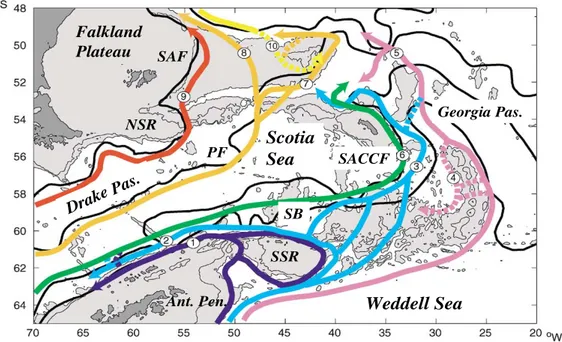
(19) The incorporation of ventilated and new formed water masses from the subpolar regions ventilates the ACC and therefore the global ocean (Orsi et al., 1999). Lateral and vertical mixing are thought to be the basic processes for the ventilation of CDW. Lateral ventilation along isopycnals was shown by Whitworth et al. (1994). Naveira-Garabato et al. (2003) obtained intense diapycnal mixing rates in the Scotia Sea (southwest Atlantic) between CDW and the upper layers of AABW from the Weddell Sea. However, it is the outflow of intermediate and deep fresher and colder Weddell Sea waters towards the Southern Boundary of the ACC that makes the Scotia Sea to play a key role in the ventilation of the Southern Ocean. CDW enters the Scotia Sea through its western boundary, the Drake Passage. Bounded north by the southern tip of the American continent and south by the South Shetland Islands, the Drake Passage forces the ACC to narrow at this longitude. After crossing the passage the ACC is bounded to the north by the Falkland Plateau and the North Scotia Ridge (NSR), and to the south by the South Scotia Ridge (SSR), both ridges running longitudinally from west to east. Whereas the gaps of the northern ridge constrain the pathways of the northern jets of the ACC (SAF and PF, Orsi et al., 1995), the gaps of the southern ridge are crucial for the ventilation of ACC waters as they allow the inflow of subpolar, ventilated waters from the Weddell Sea into the Scotia Sea (see Fig. 1.4; Naveira-Garabato et al., 2002a). The eastern boundary of the Scotia Sea is the Georgia Passage, which is much narrower than the Drake Passage as it is flanked by the South Georgia Island and the South Sandwich Islands Arc. This passage not only hosts the southern jet of the ACC (SACCF), which turns to the north at this location, but also the Southern Boundary of the ACC (Orsi et al., 1995). In the Scotia Sea, the Southern Boundary of the ACC marks the southernmost extent of CDW mixtures with Weddell Sea waters. These mixtures, which extend from the southern continental slope in the western Scotia Sea to the Georgia Passage, result in the abrupt horizontal gradients of most water properties observed in this region (see Fig. 1.4). The hydrodynamic structure of the Weddell Gyre is crucial to understand the outflow of cold ventilated waters from the Weddell Sea into the Scotia Sea. A LCDW branch of the ACC delimited by the 27.95 and 28.27 kg m-3 neutral density isopycnals (Whitworth et al., 1998) turns southwards through the Southwest Indian Ridge discontinuity (eastern. 5.

(20) boundary of the Weddell Sea; see Orsi et al., 1993) and incorporates into the cyclonic Weddell Gyre. When LCDW approaches the shelf waters of the continental margin, density gradients result in westward geostrophic currents. Along the way, mixing processes between these waters take place, eroding the core temperature and salinity maxima of LCDW and increasing the upper limit density to 28.10 kg m-3. This modified water mass is referred to as Warm Deep Water (WDW; Carmack, 1974) and occupies most of the opensea water column in the Weddell Sea. Moreover, AABW is formed in the Weddell Sea from the intrusion and mixing of SW with WDW. Defined by a neutral density > 28.27 kg m-3, it is separated into Weddell Sea Deep Water (WSDW, θ > -0.7°C) and Weddell Sea Bottom Water (WSBW, θ < -0.7°C) (Reid et al., 1977). The characteristics of AABW are conditioned by the local properties of SW (Orsi et al., 1999), but they are fresher and colder than the bottom waters of the Ross Sea, the second region in bottom water formation around Antarctica. This makes the Weddell Sea particularly important for the ventilation of the Southern Ocean.. Falkland Plateau SAF. Georgia Pas.. NSR PF. Scotia Sea. as. eP k a Dr. SACCF. SB SSR Ant. Pen.. Weddell Sea. Figure 1.4. Upper panel: scheme of the circulation in the Scotia Sea (Naveira-Garabato et al., 2002a). The fronts and some topographical features are indicated. Middle and lower panels (next page): potential temperature and salinity distributions around Antarctica at 2000m (upper level of AABW in the southern sector of the Scotia Sea, Naveira-Garabato et al., 2003). The cooling and freshening taking place in the Scotia Sea due to the outflow of Weddell Sea waters is well apparent. The higher temperatures and salinities observed in the South Atlantic correspond to NADW. Images courtesy from the WOCE Southern Ocean Atlas (http://woceatlas.tamu.edu/ ). 6.

(21) 7.

(22) The westward currents flowing along the continental margin were measured by Sverdrup (1953) at 2ºE. The associated shelf-slope frontal structures were first described by Gill (1973) at the southern rim of the Weddell Sea, and named as the Antarctic Slope Front (ASF) after the work of Ainley and Jacobs (1981). Jacobs (1986, 1991) noted that the ASF is guided by the topography and characterized by horizontal gradients in many properties across the continental slope. The ASF is found along most of the Antarctic margin, the only exception being the western coast of the Antarctic Peninsula, where CDW floods the continental shelf (Whitworth et al., 1998). At 24ºW (southeastern Weddell Sea) for instance, a single front separating inshore cold and fresh AASW from the seaward warmer and saltier WDW (the regional component of LCDW in the Weddell Sea) has been reported (see Gill, 1973). Further west, at 32ºW and 50ºW (close to the Filchner and Ronne ice shelves), a V-shaped double frontal structure filled with AASW has been reported separating the colder but saltier SW (Whitworth et al. 1998) from the offshore WDW. A sketch of the structure of the ASF is shown in Fig. 1.5.. Figure 1.5. Sketch of the Antarctic Slope Front (ASF). Image courtesy from the report of the AnSlope Program “Crossslope exchanges at the Antarctic Slope Front”, available from: http://cmdac.oce.orst.edu/data/datarpt/a nslope/planning/projdesc.pdf.. 8.

(23) After its pathway around the continental margin of the Weddell Sea, LCDW reaches again the SSR region, now on its southern flank and in the modified form of WDW. Along the northeastern slopes of the Antarctic Peninsula (Patterson and Sievers, 1980) there is a continuous mixing of colder (θmax < 0ºC; Deacon and Foster, 1977), fresher, and oxygenrich shelf waters with waters from the Weddell Gyre (θmax > 0ºC; Deacon and Foster, 1977). It is this branch of cooled and freshened Weddell Gyre waters that flows into the Powell Basin (the northernmost basin of the Weddell Sea) along its outer rim and then spreads into the Scotia Sea through the gaps across the SSR located to the west of the South Orkney Plateau (Gordon et al., 2001). A less modified inner branch continues eastwards, surrounds the South Orkney Plateau and outflows into the Scotia Sea through the gaps located to the east of the South Orkney Islands (see Fig. 1.4; Gordon et al., 2001; Naveira-Garabato, 2002a). The outflow into the Scotia Sea of Weddell Sea waters carries AASW, WDW, and WSDW. Whereas the lighter Weddell Sea waters ventilate the ACC isopycnally, WSDW underrides the ACC and diapycnally ventilates the lower layers of the ACC (Orsi et al., 1999). WSBW cannot cross the SSR and therefore it does not outflow into the Scotia Sea (Orsi et al., 1993).. 1.2. Outline of the problem As shown above, the dynamics of the Southern Ocean are key to the global ocean circulation and therefore to the Earth’s climate. On the other hand, the extreme conditions that characterize Antarctica and its surrounding ocean make this region difficult to explore and submitted to many uncertainties. One of these uncertainties is the fate of the Antarctic Slope Current (ASC) before disappearing south of the Drake Passage, after crossing the SSR (Whitworth et al., 1998). Heywood et al. (2004) traced its pathway through the southern flank of the SSR and suggested its presence in the northern wall of the Hesperides Trough. However, its incorporation into the Scotia Sea through the northern gaps of the SSR has not been documented in spite of its importance for the ventilation of the Scotia Sea. A major reason for it is that surveying the ASC is handicapped by its narrowing as the continental slope steepens to the north of the Powell Basin and by its weakening as it crosses the complicated bathymetry of the ridge region.. 9.

(24) Although the western sector of the SSR is the first outflowing gate for recently ventilated Weddell Sea waters into the Scotia Sea, the quantification of water mass transports through this region addressed in previous works showed some discrepancies. Conversely, the studies on the outflow through the eastern sector of the SSR (through the gaps located beyond the Orkney Plateau, such as the Orkney Passage) are more numerous and accurate (see e.g. Franco et al., 2007; Naveira-Garabato et al., 2002b), mainly because it was assumed that the ventilation of the Scotia Sea through the eastern SSR was more relevant than through the western sector. The outflow of WSDW through different eastern gaps is well documented, for instance, while it remains unclear for the region studied in this work. These are matters to be clarified too. The questions outlined above can only be solved by means of a dedicated survey of the region. Determining the role of the ASF and the pathway of the ASC between the South Shetland and South Orkney Islands, for instance, need of high resolution observations in order to resolve such narrow features. This was precisely one of the goals of the E-SASSI project, the Spanish contribution to the international polar year project SASSI (Synoptic Antarctic Shelf-Slope Interaction study). The main objective of SASSI was to obtain a quasi-simultaneous sampling of different continental shelf-slope regions around Antarctica, focusing on the exchanges of mass, heat, and biogeochemical parameters between the continental shelves and the open ocean. These exchanges include essential processes like the modification and formation of deep and bottom waters due to the intrusion of relative warm and salty waters over the continental shelf. The region studied by E-SASSI did not cover the regions of bottom water formation, but covered the first outflowing gate of Weddell Sea waters into the Scotia Sea. Thus, in addition to determine the role of the ASF and the pathway of the ASC between the South Shetland and South Orkney Islands, E-SASSI aimed to determine and quantify the whole outflow of Weddell Sea waters through the western sector of the SSR. The characterization of the outflow implies to study the processes involved in the modification of Weddell Sea waters as they cross this region and their interaction with Weddell Sea waters outflowing through the eastern gaps that takes place in the Scotia Sea. That is, E-SASSI was designed to characterize the contribution of Weddell Sea waters outflowing over the western sector of the SSR to the modification of the ACC and hence of the global ocean.. 10.

(25) 1.3. Objectives of this thesis The objectives of this thesis are essentially those of the E-SASSI project. We intend to reach these objectives through the analysis of the data set collected during the intensive oceanographic cruise carried out on January 2008 (the ESASSI-08 cruise). Specific objectives of this thesis are (1) to describe the regional circulation, paying particular attention to the Antarctic Slope Current; (2) to quantify the water mass transports over the western sector of the SSR; and (3) to study the modification of Weddell Sea water masses as they cross the SSR and how do they interact with Scotia Sea waters. The thesis is structured in an introduction, five major chapters and the conclusions. In this introduction we have given a brief overview of the circulation and water masses observed in the Atlantic sector of the Southern Ocean, we have defined several unknowns and set the objectives of our work. The second Chapter is a summary of the cruise carried out on January 2008 and of the subsequent data processing, paying particular attention to the calculation of the variables that are most relevant for our analysis. In Chapter 3 we use an inverse model in order to obtain a better estimation of the velocity field and hence of the transports over the ridge. The ultimate aim is a better understanding of the circulation of the different water masses and of the role of the bathymetry in the exchange of properties, aspects that are addressed in Chapter 4. Chapter 5 is devoted to determine the path and fate of the Antarctic Slope Current. The last of the major chapters (Chapter 6) focuses on the modification of Weddell Sea waters as they cross the western section of the SSR and outflow into the Scotia Sea. In particular we determine the water mass fractions of the modified water masses present in the region by applying an Optimum Multiparameter Technique. The main conclusions of this work are outlined in Chapter 7.. 11.

(26) 12.

(27) CHAPTER 2 THE ESASSI-08 CRUISE AND DATA TREATMENT. 2.1. The ESASSI-08 cruise In the framework of the recent International Polar Year, the ESASSI-08 cruise was carried out on January 2008 on board R/V Hespérides. Of the 20 scientists onboard the vessel, 15 were from the Mediterranean Institute for Advanced Studies (IMEDEA), 4 from the Texas A&M University (TAMU), and 1 from the University of East Anglia (UEA). A team of 8 technicians from the Marine Technology Unit (UTM) of the Spanish National Research Council (CSIC) was responsible for the logistics of the measurements. After sailing from Ushuaia (Argentina) on January the 2nd, and before crossing the Drake Passage, the main task was the calibration of the ship-borne Acoustic Doppler Current Profiler (ADCP). The calibration based on changing the heading by 90º from one transect to another, for a total of 5 transects of about 20 minutes each. The aim was to align correctly the instrument respect to the hull of the vessel. Besides, a hydrographical cast was made to test the Conductivity-Temperature-Depth (CTD) sensor. The survey of the target region started the 4th of January and it covered the Weddell-Scotia Confluence region, from 60ºS to 62ºS and from 58ºW to 46ºW. The design of the sampling was planned in order to address the questions outlined in the previous section, namely the path of the Antarctic Slope Current over the western sector of the South Scotia Ridge and the export of waters from the Powell Basin to the Scotia Sea. A total of 113 CTD profiles were obtained, distributed along 11 sections running across different slopes of the SSR and along three additional transects (see Fig. 2.1 and Table 2.1). All cross-slope sections followed a similar strategy: one or two casts were obtained over the continental shelf; the others where obtained at different depths downslope, with a separation distance decreasing down to 2 nm where the sharp gradients characteristic of the slope front where detected. The CTD profiles (including those obtained by the attached oxygen and fluorescence sensors) run from surface to bottom at every station. Discrete water samplings were also taken at different depths with the aim of calibrating the CTD sensor and to measure a whole set of biogeochemical parameters. 13.

(28) o 8 5 S. Scotia Sea Drake Pas.. o. 59 S. Shackleton Fracture. o. T1. 60 S S1. Elephant Is.. 61 S. T3. S7. o. 63 S o. S tr d l ie nsf a r B. 64 S o 60 W. ait. 1500m 2500m. Antarctic Peninsula. o. South Orkney Is. and Plateau. S9 Philip 8 S Pas.. Powell Basin. o. 62 S. Orkney Pas.. T2. S4. S2. o. Hesperides Pas. S10. S3 S5N S5 S6. 56 W. Weddell Sea. o. 52 W. o. 48 W. 44 oW. 4 0oW. Figure 2.1. The ESASSI-08 hydrographic sampling (transects and transit casts in red; yo-yo station in green). The bathymetry is from Smith and Sandwell (1997); the areas shallower than 1000m are shaded.. 14.

(29) Table 2.1. Tracking of the ESASSI-08 cruise. Sections and transits Beagle Channel. Starting position Starting date Ending position Finishing date Port of Ushuaia. Cast. 02/01/08 11:00 55º18’S 66º20’W 03/01/08 01:00. Calibration of the ship-borne ADCP. 55º18’S 66º20’W 03/01/08 05:21 55º28’S 66º19’W 03/01/08 07:06. Drake Passage. 55º31’S 66º14’W 03/01/08 08:09 60º44’S 57º08’W 04/01/08 22:19. Section S1 (south of Drake Passage). 60º48’S 57º04’W 04/01/08 22:48 61º05’S 56º03’W 05/01/08 21:31. Transit from section S1 to section S2. 61º05’S 56º03’W 05/01/08 21:31 61º04’S 54º49’W 06/01/08 02:34. Section S2 (north of Elephant Island). 61º04’S 54º49’W 06/01/08 02:34 60º47’S 54º47’W 06/01/08 19:28. 09-15. Transit T1, from section S2 to section S3 (Scotia Sea). 60º47’S 54º47’W 06/01/08 19:28 60º09’S 52º42’W 07/01/08 11:49. 16-17. Section S3 (cross-slope section in the Scotia Sea). 60º09’S 52º42’W 07/01/08 11:49 60º25’S 52º53’W 08/01/08 05:13. 18-24. Section S4 (gap of the northern flank of the SSR). 60º27’S 52º41’W 08/01/08 08:53 60º22’S 52º01’W 09/01/08 09:43. 25-35. Section S5N (cross-slope section in the Scotia Sea). 60º22’S 52º01’W 09/01/08 09:48 60º07’S 51º52’W 10/01/08 08:12. 36-44. Transit from section S5N to section S7. 60º07’S 51º52’W 10/01/08 08:12 61º22’S 51º32’W 10/01/08 19:15. Section S7 (cross-slope section in the Weddell Sea). 61º22’S 51º32’W 10/01/08 19:15 61º33’S 51º15’W 11/01/08 14:53. Transit from section S7 to section S8. 61º33’S 51º15’W 11/01/08 14:53 61º17’S 51º15’W 11/01/08 18:28. Section S8 (gap of the southern flank of the SSR). 61º17’S 51º15’W 11/01/08 18:28 61º06’S 50º36’W 12/01/08 21:30. 54-68. Section S9 (cross-slope section in the Weddell Sea). 61º06’S 50º36’W 12/01/08 21:30 60º57’S 50º02’W 13/01/08 09:50. 69-75. 15. 00. 01-08. 45-53.

(30) Transit T2, from section S9 to section S6 (Hesperides Trough). 60º57’S 50º02’W 13/01/08 09:50 60º13’S 50º03’W 14/01/08 05:10. 76-78. Section S6 (cross-slope section in the Scotia Sea). 60º13’S 50º03’W 14/01/08 05:10 60º03’S 50º02’W 14/01/08 17:40. 79-85. Transit from section S6 to section S5. 60º03’S 50º02’W 14/01/08 17:40 60º17’S 51º19’W 15/01/08 02:58. Section S5 (gap of the northern flank of the SSR). 60º17’S 51º19’W 15/01/08 02:58 60º13’S 50º25’W 15/01/08 16:49. Transit from section S5 to section S10. 60º13’S 50º25’W 15/01/08 16:49 60º13’S 49º19’W 15/01/08 22:35. Section S10 (Hesperides Passage). 60º13’S 49º19’W 15/01/08 22:35 60º12’S 47º02’W 16/01/08 22:45 94-100. Transit from section S10 to Signy Is. (South Orkney Islands). 60º12’S 47º02’W 16/01/08 22:45. Transit from Signy Is. to the yo-yo station. Signy. Signy. 86-93. 18/01/08 04:30. 18/01/08 05:00 61º15’S 51º13’W 19/01/08 16:55. Yo-yo station. 61º15’S 51º13’W 19/01/08 16:55 61º15’S 51º16’W 20/01/08 04:31 101-111. Transit T3, southwestern flank of the SSR. 61º15’S 51º16’W 20/01/08 04:31 61º14’S 53º19’W 20/01/08 17:16 112-113. Transit from the last station to Deception Island. 61º14’S 53º19’W 20/01/08 17:16 Deception Island. 16.

(31) 2.2. Data set and instrumentation The rosette used in the ESASSI-08 cruise hosted a Seabird 911 CTD and 24 Niskin bottles of 12 l each for water samplings. The down/up casts were carried out at a speed between 45 and 60 m min-1 and were controlled from an onboard computer. In this way CTD measurements were observed in real time and the depth of the bottle samples (taken during the upcasts) were decided looking at the downcast profiles. The variables measured by the CTD multisensor were conductivity, temperature, and pressure, but the acquisition software also provided salinity (inferred from conductivity), density (inferred from temperature, salinity and pressure using the state equation) and depth (inferred from the vertical integration of the specific volume with pressure). Dissolved oxygen, turbidity, and fluorescence were also measured with additional sensors attached to the CTD. The water samples from the bottles provided accurate measurements of salinity, dissolved oxygen and chlorophyll, which were used for the calibration of the conductivity, oxygen, and fluorescense sensors of the CTD, respectively. Clorofluorocarbons (CFC), nutrients (silicates, phosphates, nitrates) and other biogeochemical parameters such as pH, alkalinity or dissolved organic carbon were also measured from the water samples. Phosphates will be used in this work as water mass tracers. The vessel-mounted ADCP measures the speed and direction of currents relative to the ship (in which case the ship velocity must be accurately determined in order to infer absolute current velocities) or relative to the bottom (only in waters shallower than 500m approximately). The vertical resolution and range of the measurements depends on the accoustic frequency: higher frequencies result in a higher vertical resolution, but in a shorter vertical range. For the ESASSI-08 cruise the ADCP was set to provide measurements in 8m vertical cells covering from surface to about 600m depth. Data were collected both at stations and along the track of the ship. The accuracy of a single profile was estimated in 0.09 m s-1 in the upper 450m and in 0.17 m s-1 from 450m to 600m. The accuracy can be improved by averaging a set of velocity profiles: for the ESASSI-08 cruise we averaged the profiles in 20-min intervals (i.e., over 2 nm along track), which in the best case would resulted in an accuracy of the order of 0.02-0.03 m s-1.(errors can be significantly larger due to inaccuracies in the navigation system, for instance).. 17.

(32) Additional measurement were those provided by a thermosalinograph measuring in a continuous way a flow of water sucked from 4 - 5m depth. The same flow was used to measure also CFCs and other parameters. Data from the meteorological station, different acoustic echo-sounders, and the navigation systems (GPS, heading, velocity of the ship) were all acquired in an automatic mode and saved by the System for Oceanographical Data Adquisition (SADO) installed onboard. Not all the variables have the same spatial resolution. The variables saved by the SADO and the ship-borne ADCP cover most of the track of the ship, though in the case of the ADCP they only cover the upper (600m) levels. Data from the CTD and the attached oxygen, fluorescence and transmittance sensors are discrete in the horizontal dimension (they were acquired only at station points) but are continuous in the vertical and cover from the surface to the bottom. The water samples from the Niskin bottles are discrete in both, the horizontal dimension (they were sampled at every CTD station) and in the vertical dimension (the samples were obtained typically at 10-12 levels in the vertical). The range of measurement of the temperature sensor of the CTD is from -5ºC a +35ºC, with a nominal accuracy of ±0.001 ºC and a resolution of ±0.0002 ºC. Although this sensor can hardly be calibrated from cruise measurements, it is considered to be quite reliable provided it is routinely calibrated in between cruises (as it was the case). The pressure sensor used in ESASSI-08 had a nominal accuracy of ±0.015% and a nominal resolution of ±0.001% of the whole measurement range, which was of 10500m (i.e., an accuracy of about 1.5m and a resolution of about 0.1m). The nominal accuracy and resolution of the conductivity sensor expressed in practical salinity units were ±0.001 and ± 0.0002, respectively. Unlike the temperature sensor, the conductivity cell is more sensible to drifts due to environmental conditions, and therefore a calibration against water sample salinity measurements is highly recommended. The same applies to the dissolved oxygen sensor. The calibration procedures and their results are presented in the following.. 18.

(33) 2.3. Calibrations. 2.3.1. Conductivity sensor A total of 258 salinity samples were analyzed onboard with an autosalinometer, a Guildline Portasal 8410A calibrated with IAPSO Standard Seawater ampoules. The measurement range of that model is from 2 to 42, the accuracy is ±0.003 and the resolution is ±0.0003. Although the nominal accuracy of the salinometer is worse than the accuracy of the conductivity sensor of the CTD, the latter is more submitted to drifts and therefore an in situ calibration against the water samples is highly recommended. Water sample salinity measurements covered a wide range of stations and depths, recording values from 34.1 to 34.8. The linear regression between water samples and CTD values gave a correlation coefficient of 0.9991 and a mean value for the residuals of ±0.003, which is within the value of the nominal accuracy of the autosalinometer (Fig 2.2). Hence, no further correction apart from the linear regression towards the water samples was applied to salinity CTD data.. 34.8 34.7. Sautosal = (0.9938 ± 0.0019) SCTD + (0.22 ± 0.06) 2. R = 0.9991 RMS = ± 0.003. Sautosal. 34.6 34.5 34.4 34.3 34.2 34.1 34.1. 34.2. 34.3. 34.4. 34.5. SCTD Figure 2.2. Linear regression for the salinity data sets.. 19. 34.6. 34.7. 34.8.

(34) 2.3.2. Dissolved oxygen sensor. The accuracy and resolution of the oxygen sensor are significantly poorer (relative to the usual variability of the parameter) than for the conductivity or the temperature sensors. This makes the calibration of that sensor to be particularly important. Bottle water samples were analyzed by applying the Winkler methodology, a potentiometric titration method (Culberson and Huang, 1987) where the 0.01N iodate OSIL standards were used for quality control following the recommendations of Culberson et al. (1991) for aliquot determinations. The analysis of replicate samples taken from the same Niskin bottle point to a precision of less than 0.7 µmol kg-1 for dissolved oxygen. A preliminary analysis of the first 28 stations revealed important differences between the values measured by the CTD sensor and the Winkler measurements (Fig. 2.3). A comparison with historical data in the Scotia Sea, the differences between the downcasts and upcasts and other calibration tests suggested that the Winkler measurements are correct, so that the problem was with the oxygen sensor of the CTD. In particular it seems that the sensor experienced a hysteresis with pressure during the first part of the cruise, perhaps because it was a new sensor (Fig. 2.4). For the other casts (29-113) the values given by the CTD sensor are more in agreement with the Winkler measurements. In that latter case the calibration of the oxygen sensor data set is straightforward, as a simple linear regression is enough for these values to match the water sample measurements. The calibration of the station 1-28 data set is more problematic, as it can be inferred from Fig. 2.4, which shows higher and pressure dependent residuals for the first water sample batches. We first tried a regression with an exponential dependence with pressure, in an attempt to eliminate the observed anomalies. After that, two mean square linear regressions were applied to the residuals, one for the data located between 100 and 900 db and another one for pressures greater than 900 db. For the upper range 0-100 db results were not satisfactory and therefore they were discarded; this is not a great loss, since surface oxygen velocities are not as important as at deeper levels for the study of water masses.. 20.

(35) 380 360. O2 Winkler (µmol kg-1) O2 winkler. 340 1 2 3 4 5 6 7 8 9 10 11 12 13 14. 320 300 280 260 240 220 200 180 160 160. 180. 200. 220. 240. 260 280 300 O2 CTD (µmol kg-1). 320. 340. 360. 380. O2 CTD. O2 residuals (µmol kg-1) Res O2. Figure 2.3. Comparison of dissolved oxygen values given by the oxygen sensor of the CTD and the Winkler results. ‘Batchs’ are sets of water samples analyzed altogether and that include different casts. The most important deviations correspond to casts from 1 to 28 (batches 1, 2, 3, and part of 4). Figure courtesy of M. Álvarez.. 100. 0. -100. casts All 1 to 28 castsBatch>=4 29 to 113. -200. 0. 2. 4. 6. 8. 10. 12. 14. Res O2 O2 residuals (µmol kg-1). Batch 100 50 0 -50 -100 -150. 0. 500. 1000. 1500. 2000 2500 3000 Prs (db) Pressure. 3500. 4000. 4500. Figure 2.4. Differences between Winkler and CTD oxygen measurements after applying a common linear regression to the data set (black line in Fig. 2.3). The residuals are smaller and independent on pressure for casts 29-113 (batch>4). The residuals are larger and dependent on pressure for casts 1-28 (batch 1-4).. 21.

(36) The numerical expressions used to calibrate the CTD dissolved oxygen are:. Casts 1 to 28: R2 = 0.70, RMS = 14 µmol kg−1  O2 Winkler = ( 381± 6) p( −0.065±0.003) + (1.03± 0.07) O2 CTD + ( −226 ±17) , 100db ≤ p<900db  −1 O2 ( µmol kg ) R2 = 0.76, RMS = 7 µmol kg−1  −0.065±0.003) + ( 0.63± 0.05) O2 CTD + ( −150 ±11) , p ≥ 900db O2 Winkler = ( 381± 6) p(  −1 O2 ( µmol kg ) Casts 29 to 113: R2 = 0.99, RMS = 4 µmol kg−1  O2 Winkler = (1.237 ± 0.007) O2 CTD + ( −3.7 ±1.4) , p( db)  −1 O2 ( µmol kg ) Although the correction has significantly reduced the differences between Winkler and CTD values, the first 28 casts must be taken with caution. When plotting vertical sections of the different parameters and after a water mass analysis we conclude that calibrated oxygen data from casts 1 to 28 are good enough, but not excellent. For instance, no reliable trends can be inferred from the comparison with other cruises in the region. Conversely, the accuracy of the other casts (29-113) and the bottle values of the first casts (1-28) are valid to be used for any purpose.. 2.3.3. Phosphate measurements Samples for phosphate analysis were saved in high-density polyethylene tubes and frozen. They were analyzed at IMEDEA using a Bran-Luebe AA3 autoanalyzer and following standard methods (Hansen and Koroleff, 1999). When comparing the obtained phosphate concentrations with historical data from the WOCE Southern Ocean Atlas (Orsi and Whitworth, 2005), a bias of -0.65 ± 0.15 µmol kg-1 was detected and corrected (see Fig. 2.5).. 22.

(37) Figure 2.5. Neutral density vs. phosphate concentrations. ESASSI direct measurements (red) and climatological values (black).. As part of the nutrient cycle, organic phosphates are re-mineralized by bacteria in the water column: ∆ ( PO 4 ) = PO 4* − PO 4 . Broecker et al. (1998) stated that the ratio between the phosphates and oxygen used by bacteria during this process ( ∆ ( O 2 ) = O 2saturation − O2 ) is approximately constant: -. ∆ ( O2 ) ∆ ( PO 4 ). = 175 . This allows the estimation of PO 4* , which can. be used as a quasi-conservative tracer of water masses (see e.g. Naveira-Garabato et al., 2002b). We will examine the distribution of PO 4* later on in this work.. 2.4. Neutral density The basic physical parameters to classify water masses in the ocean are potential temperature, salinity, and neutral density. Salinity is given by the acquisition software of the CTD. The computation of potential temperature (the temperature of a water parcel. 23.

(38) when it is adiabatically moved from its original position to the surface) is straightforward; we used the CSIRO MatLAB Seawater Library (Phil Morgan, maintained by Lindsay Pender, 2003) based on the UNESCO algorithms. Instead, some background related to different density variables (Stewart, 2005) is needed to better understand the meaning of neutral density. The absolute density is difficult to measure out of the environmentally controlled conditions of a laboratory. The use of a density relative to the density of pure water is consequently more extended. The “in situ” density is the density of a water parcel at a certain depth. It is a function of salinity, temperature, and pressure: ρ = ρ ( S, T, p ) . Due to the small changes in sea water, the density anomaly σ ( S, T, p ) = ρ ( S, T, p ) − 1000 kg m −3 is more widely used. When it comes to compare water masses, however, it is necessary to reference the density to the same pressure level, in order to avoid density differences due to the effects of pressure. A water parcel can be denser than another parcel of the same water mass just because it is located at a different pressure level. At upper levels the surface pressure can be used as reference, the density then being computed as σ t = σ t ( S, T, p = 0 ) . At levels deeper than a few hundred meters, however, the warming due to the effects of pressure is no longer negligible and must be taken into account. Most of this indirect effect of pressure over the density is eliminated by using the potential temperature θ instead of the in situ temperature in the density equation: σθ = σθ ( S, θ, p = 0 ) . This approximation is the so called potential density and it eliminates not only the direct effect of pressure over the density, but also the indirect effects through temperature. There are still other effects not considered by the definition of σθ which can be relevant at depths greater than a thousand meters and for long trajectory water masses. That is the case of the Southern Ocean, where it is convenient to use of a more appropriate definition of density. When analyzing the properties of the ocean to determine the origin of water masses, it is assumed that the movement of a water parcel located in the interior of the ocean is mostly due to the density distribution. This implies that a water parcel follows a layer of heat (isentropic surface) and salt conservation. This type of surface is complicated to define when mixing processes are involved. In practice, potential density surfaces are often used to trace the path of a water parcel. Thus, from 0 to 500db, the isentropic surfaces are 24.

(39) approximated by the potential density computed relative to the surface (σ0); from 500 to 1500 db, potential density surfaces referred to 1000 db (σ1) are used; and so on. This method is obviously better than using σ0 at all depths, but it is not perfect for a wide range of pressure levels. Jackett and McDougall (1997) published a key paper where they defined a new variable, the neutral density. Neutral density surfaces are the closest approximation to the real isentropic surfaces and are almost globally described. They are based on the interpolation of an extensive data set of CTD profiles and water samples around the globe, all it implemented in a package that can be easily applied to the most extended programming languages. The neutral density is a function of latitude, longitude, pressure, in situ temperature, and salinity, and has an error (derived from the interpolation) smaller than the observational error.. 2.5 De-tiding of ADCP measurements ADCP measurements were taken along the track of the ship shown in Fig. 2.6. In order to evaluate the potential impact of tidal currents on hydrographic data, a yo-yo station located at the shelf break of section S8 (600m depth, see Fig. 2.6) was also performed during the cruise. Figure 2.7 (upper panel) shows the sequence of temperature profiles gathered during 12 hours at that station. There is a clear transition from profiles that are characteristic of shelf waters (more homogeneous) to profiles that reflect the structure of open ocean water masses (with a subsurface temperature minimum characteristic of remnant WW located at 100-200m and the 400-500m temperature maximum characteristic of WDW). These results suggest that WDW could flood and retreat from the slope region with a tidal periodicity. The tidal currents measured at the yo-yo station were as high as 1 m s-1 (see Fig. 2.6, lower panel). Similar values were obtained over the shelf-slope of some of the other gaps surveyed during the cruise. This unexpected feature (previous studies had reported weak tidal currents in the region) confirms the crucial role of the abrupt bathymetry in the forcing of the flow. Regarding the data processing, it makes clear that ADCP data must be carefully detided if they have to account only for the subinertial flow. In order to eliminate tidal currents from the ADCP record, we tested three models: the circum-Antarctic inverse barotropic tidal model (CADA, Padman et al., 2002), the Antarctic. 25.

(40) o. Scotia Sea. 58 S. Drake Pas.. o. 59 S. Shackleton Fracture T1. o. 60 S. S3 S5N S4. S5. S1. 61 S o. 62 S o. 63 S o. S th u So. d an l t he. Is.. T3. S7. South Orkney Is. and Plateau. S9 Philip 8 S Pas.. Powell Basin. it tra S d fiel s n Bra. 64 S o 60 W. Orkney Pas.. T2. S2. o. Hesperides Pas. S10. S6. 1500m 2500m. Antarctic Peninsula. o. 56 W. Weddell Sea. o. 52 W. o. 48 W. 44 oW. 4 0oW. Figure 2.6. ADCP data set along the ship tracking (blue). ESASSI-08 hydrographic sampling (transects and transit casts in red; yo-yo station in green). The bathymetry is from Smith and Sandwell (1997); the areas shallower than 1000m are shaded.. 26.

(41) 0 100. Eastward velocity (m s-1). -0.6. -0.4 θ (ºC). 1. 0. -1. -2 0. ADCP CADA CATS2008b ANTPEN. 2. 4. 6 8 Hours. 10. -0.2. 0. 0.2. 0.4. 106 107 108 109 110 111. -0.8. 104 105. -1. 102 103. 101. 700 -1.2. 101. 600. Northward velocity (m s-1). 500. 106 107 108 109 110 111. 400. 101 102 103 104 105 106 107 108 109 110 111. 104 105. 300. 102 103. p (db). 200. 1. 0. -1. -2 0. ADCP CADA CATS2008b ANTPEN. 2. 4. 6 8 Hours. 10. Figure 2.7. Upper panel: temperature profiles measured at the ESASSI yo-yo station located at the shelf break of section S8 (depth of 600m, see Fig. 2.6 for location). Lower panels: mean velocity components obtained by vertically averaging ADCP data gathered below a depth of 50m (black line, with the standard deviation from the mean value in gray) and tidal velocity components at the same location and time as predicted by three tide models; the time at which the profiles of the upper plot were gathered is marked.. 27.

(42) Peninsula high-resolution tidal forward model (AntPen, a regional version of CATS, Padman et al., 2002), and a recent update of the circum-Antarctic tidal forward model CATS02 (CATS2008b, Padman et al., 2008). The three models gave very similar results at open-sea. At section S8 (Fig. 2.7) the overall structure of the tidal current given by the three models is also similar and consistent with the directions inferred from the hydrographic profiles obtained along the section. However, the magnitude of the currents is rather different among the models, particularly over the shelf break. After a careful checking of the model outputs against sea level data and an exhaustive comparison of the vertical structure of the residual currents against geostrophic currents, the AntPen model was chosen for the de-tiding.. Figure 2.8. Velocity components and velocity speed estimated by vertically averaging ADCP data gathered below 50m plotted along the track of the ship (black line, with the standard deviation from the mean value in gray). Tidal velocity components and speed at the same location and time as predicted by the AntPen model (red line). The location of the sections plotted in Fig. 2.6 is marked.. 28.

(43) Figure 2.8 shows the mean velocities estimated from ADCP data along the whole track of the ship. The values were obtained averaging the layer below 50m in order to avoid windinduced effects (tidal currents are essentially barotropic, as inferred from the small deviations from the mean shown in Fig. 2.7). Figure 2.8 also shows the collocated tidal currents given by the AntPen model. Altogether, results suggest that tidal currents are the dominant component of the flow; the highest speeds are observed at the southern flank of the ridge (sections S7, S8 and S9, and at transit T3, from S7 to Elephant Island).. 2.6 Baroclinic and barotropic components of the flow Ocean dynamics is described by the momentum equations for horizontal velocities, and the hypothesis of hydrostatic balance and incompressibility. Because the ocean interior is very approximately in geostrophic balance, the prognostic equations can be reduced to the diagnostic equations giving the longitudinal and latitudinal geostrophic velocities (Ug , Vg).. 1 ∂p = fVg ρ ∂x. ;. 1 ∂p = − fU g ρ ∂y. (2.1). where p is pressure, ρ is density, f is the Coriolis parameter, g is the gravity acceleration and (x,y) are the horizontal coordinates. Having the stations distributed along cross-slope sections implies that only the cross-section (along-slope) flow can be obtained. The geostrophic velocity field can be split into two components: the baroclinic and the barotropic components. The first one gives the velocity shear with respect to a reference level and depends on the contribution of horizontal density differences to the pressure gradients appearing in (2.1). In a finite differencing scheme and working with pressure instead of z as vertical coordinate, the cross-section baroclinic component of the geostrophic flow (Vbc) in between two (station or grid) points can be expressed simply as the difference between the dynamical height (Φ) measured at these two points divided by the distance between the points (∆x) and the Coriolis parameter (see e.g. Stewart, 2005):. Vbc ref =. 10 d Φ ref 10 Φ ( x + ∆x ) ref − Φ ( x ) ≃ f dx f ∆x 29. ref. (2.2).

(44) A second contribution to the horizontal pressure gradients appearing in (2.1) comes from sea level height anomalies. In this case the pressure differences (and hence the derived geostrophic velocity) will be the same at every depth. This is the barotropic component (Vbt) of the flow. The baroclinic component of the flow can be estimated at any depth where T, S (and hence density) measurements are available. On the other hand, (absolute) velocity measuremets (Vabs) are only available for the depth range covered by the ADCP (upper several hundred meters). Thus, if we take advantage of the two independent data sets (density and velocity) covering the upper levels to estimate the barotropic component, this could also be added to the baroclinic component computed below the range of the ADCP in order to recover the absolute velocity at any depth. The important point to be noticed is that the barotropic component is constant with depth, and therefore the value computed at upper levels is the same to be added at lower levels. It is also important to note, however, that since the baroclinic component depends on the reference level used for the geostrophic computations, the barotropic component will also be a function of that level:. Vabs ( p ) = Vbc ( p ) p + Vbt ( pref ref. ). (2.3). In principle, Vbt(pref) could be determined using velocity measurements at any single level. p, since (2.3) is valid everywhere. In particular, since Vbc(pref)│pref = 0, the barotropic component could be simply made equal to the actual velocity field at the reference level (Chereskin and Trunnell, 1996). The problem is that the noise-to-signal ratio of ADCP data is rather high. Although the nominal accuracy reported in section 2.2 for averaged ADCP profiles was quite acceptable, it neglects for instance the errors derived from inaccuracies in the detiding process. Thus, using (2.3) as it stands would imply transferring the errors of ADCP data to the barotropic component of the flow Vbt(pref). It can be shown, for instance, that using (2.3) at different p levels would result in rather different Vbt(pref) estimates. Rudnick (1996) suggested to determine the barotropic component in a different way, namely through the minimization of the expression. (V ( p ) − V abs. ADCP ( p ) ). 30. 2. (2.4) ADCP range.

(45) where the overbar could in principle denote vertical averaging over the ADCP range. This is equivalent to make the barotropic component equal to:. Vbt ( pref ) = VADCP ( p ) − Vbc ( p ) p. (2.5). ref. That is, the optimal value of Vbt(pref) would be that minimizing the differences between absolute geostrophic velocities and the observed velocities. The basic assumption of Rudnick’s method is that the vertical averaging of the differences between ADCP and the baroclinic component is more reliable than the same difference evaluated at a single level, as proposed by Chereskin and Trunnell (1996). This is likely to be the case in the presence of random errors, but it is also clear that the method will not prevent the pouring of vertically correlated ADCP errors into Vbt(pref). Another advantage is the independence of the estimated absolute geostrophic velocities with respect to the choice of the reference level, a property that can be easily proved from:. Vabs ( p ) = Vbc ( p ) p + VADCP ( p ) − Vbc ( p ) p ref. ref. (2.6). A hypothesis implicit in Rudnick’s method is that the flow is essentially geostrophic. Because this can only be ensured in the ocean’s interior, it is advisable that the averaging domain of (2.4)-(2.6) ignores the surface Ekman layer. For the method to work properly it is also crucial that the a-priori de-tiding of ADCP velocities is as accurate as possible. Another quality control applied prior to the application of Rudnick’s method consisted of checking the consistency between adjacent CTD stations, particularly over the shelf break. A few ESASSI stations located very close to their neighbours (e.g. casts 13, 26, 31, 34, 49, 88) were discarded on the basis of the comparison between the vertical structure of the detided currents and the geostrophic currents between stations. The misfit obtained at the discarded station pairs is due to the lack of synopticity and to the application of the geostrophic balance to structures smaller than the Rossby radius of deformation. Although the lack of synopticity also affects station pairs separated by longer distances, the impact on the mean geostrophic velocity is less important than for stations located very close to each other.. 31.

(46) After the estimation of the absolute geostrophic velocity field, computing the cross-section geostrophic flow is, in principle, straightforward. Specific details such as the downwards extrapolation of the velocity field over the slope will be discussed in the next chapters.. 32.

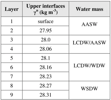
(47) CHAPTER 3. GEOSTROPHIC VELOCITY AND TRANSPORTS FROM AN INVERSE MODEL. In this chapter we present an accurate quantification of the transport of volume, heat, and salt through the gaps of the SSR west of the South Orkney Islands. Absolute velocities are first estimated from the CTD casts and ship-borne ADCP data described in the previous chapter. This first estimation is then used as a first guess for the inverse model. The design of the inverse model is presented in section 3.1, while the setup is presented in section 3.2. In section 3.3 we present the application of the model and the analysis of its impact on the first guess of the velocity field. The analysis of the results in terms of the regional circulation (water mass pathways and associated transports) is addressed in chapter 4.. 3.1. Inverse model design Inverse modeling (Wunsch, 1977) allows correcting the velocity field by applying flow conservation equations to a set of neutral density layers of the water column within an enclosed region of the ocean assumed to be in geostrophic balance. For this work, we use the DOBOX model, implemented by Morgan (1994) and tested against a numerical model by McIntosh and Rintoul (1997). The layers considered in this work (see Table 3.1) were chosen basing on the separation between the different water masses present in the region.. 3.1.1. Box domain The domain for the inversion covers from 60˚S (the northern flank of the SSR) to 61.5˚S (the southern flank) and from Elephant Island to 50˚W (Fig. 3.1). The box makes use of six of the hydrographic sections sampled during the ESASSI-08 cruise, with closely spaced stations (1-2 nm over the slope, less than 5 nm elsewhere, 1nm ≡ 1852 m) covering the main passages of the northern and southern flanks of the SSR. The box also uses three transits extending along greater distances but with fewer stations. Direct current measurements from a ship-borne ADCP were collected along all the sections and transits.. 33.

(48) Table 3.1. Inverse model layers and water masses delimited by the chosen neutral density surfaces. Layer. Upper interfaces γn (kg m-3). 1. surface. 2. 27.95. 3. 28.0. 4. 28.06. 5. 28.1. 6. 28.16. 7. 28.23. 8. 28.27. 9. 28.31. Water mass AASW LCDW/AASW. LCDW/WDW. WSDW. The most important gaps crossed by the box model are the two westernmost gaps of the southern flank (2100m and 2500m depth, sections S8 and S9, respectively), the Hesperides Trough (4000m depth, northern part of transit T2), and the two westernmost gaps of the northern flank (1700m and 1300m depth, sections S4 and S5, respectively). The ESASSI08 cruise did not cover the stretch between Elephant and Clarence Islands, and from Clarence Island to the beginning of transit T3. The closure of the box at this site is addressed in the next section.. 3.1.2. Closure of the box The last hydrographic station of the ESASSI-08 cruise (cast 113, see Fig. 3.1) is located about 80 km to the E-SE of Elephant Island. No ADCP data were recorded between that cast and Elephant Island. Some inflow from the Bransfield Strait has been reported to enter the selected domain through that gap (López et al., 1999) and therefore it must be included in the conservation equations before the inversion of the model equations. The estimation of the property transports across that transect will be based on historical data and on previous results obtained by other authors.. 34.

(49) Drake Passage. Hesperides Gap and Trough. Section 3. Section 5. 18. o. 60 S. Transit 1. Shackleton Fracture. 30'. 79. 17. 78. 16. 32. 24. 36. Section 2. 61 S. Elephant and Clarence Is.. 30'. 112. 69. Philip Passage. Section 9. 58 62. 113. Transit 3. Section 8. South Orkney Is.. South Orkney Plateau. Powell Basin. o 62 S. 30'. 76 65. 9. Orkney Passage. Transit 2. 77. Section 4. 15. o. Scotia Sea. 91. Bransfield Strait. 1500 m. Antarctic Peninsula. o 63 S. o 56 W. Weddell Sea 52oW. 48 oW. 2500 m. 44 oW 40 oW. Figure 3.1. ESASSI-08 hydrographic stations (red crosses) in the region. The stations constituting the model box are linked; only the most relevant are numbered. The bathymetry is from Smith and Sandwell (1997); the areas shallower than 1000m are shaded. The topographical gaps crossed by the boundaries of the model domain have been encircled: one of them is in the southern flank of the South Scotia Ridge (section S8) and two in the northern flank (sections S4 and S5). The eastern boundary of the box (transit T2) runs from the southern flank to the northern flank.. 35.

(50) A relevant contribution to the knowledge of the missing transect comes from the hydrographic data collected during the ECOANTAR-94 cruise carried out in January 1994. That is, the same month as the ESASSI-08 cruise, though 14 years earlier. During ECOANTAR-94 the whole eastern basin of the Bransfield Strait was covered with a regular distribution of stations spaced 20 km (López et al., 1999). Those hydrographic data and the baroclinic component of the geostrophic velocities computed with respect to the deepest common level enable the tracking of the water masses exiting the Bransfield Strait to the east, since they cover most of the gap of the ESASSI-08 cruise. The barotropic component of the current cannot be estimated from ECOANTAR-94 data, due to the absence of direct current measurements. Instead, absolute velocities were estimated from near surface velocities recorded by drifters and interpolated over the ECOANTAR94station pairs. The analysis of the data set of historical and ADELIE-07 drifters provided by Thompson et al. (2009) shows a negligible barotropic component compared with the geostrophic shear. The ECOANTAR-94 stations cover most of the missing transect, but there is still a small uncovered segment shallower than 500m close to the southeast coast of Elephant Island. The hypothesis we make is that the westward flow observed at the northern coast of the island (casts 9-10, section S2) is a coastal current surrounding Elephant Island anticlockwise, so that the volume transport at the southern coast should be equal to the transport observed to the north of the island. A previous study of the ECOANTAR-94 cruise (López et al., 1999) estimated the geostrophic flow across the missing transect in approximately 0.5 Sv, of which 0.4 Sv would enter the box domain between Elephant and Clarence Islands and 0.1 Sv would enter the box to the southeast of Clarence. That calculation is based on the hypothesis of a common level of no motion at 500m depth. A re-calculation down to the bottom and the inclusion of the coastal flow around Elephant Island increase the net volume transport up to 1.4 Sv (Table 3.2). The lack of synopticity between the drifters and ECOANTAR-94 data as well as the inherent temporal variability of the Bransfield currents (Savidge and Amft, 2009) suggest considering transport uncertainties of the same order as the quoted absolute values.. 36.