Long run efficiency of price structures in hydrothermal electric systems

Texto completo

(1)PONTIFICIA UNIVERSIDAD CATOLICA DE CHILE ESCUELA DE INGENIERIA. LONG RUN EFFICIENCY OF PRICE STRUCTURES IN HYDROTHERMAL ELECTRIC SYSTEMS. HEINZ MÜLLER. Thesis submitted to the Office of Research and Graduate Studies in partial fulfillment of the requirements for the Degree of Master of Science in Engineering. Advisor: HUGH RUDNICK. Santiago de Chile, (June, 2012)  2012, Heinz Müller, Alexander Galetovic, Cristian Muñoz, Hugh Rudnick..

(2) PONTIFICIA UNIVERSIDAD CATOLICA DE CHILE ESCUELA DE INGENIERIA. LONG RUN EFFICIENCY OF PRICE STRUCTURES IN HYDROTHERMAL ELECTRIC SYSTEMS. HEINZ MÜLLER Members of the Committee: HUGH RUDNICK ALEXANDER GALETOVIC CRISTIAN MUÑOZ DAVID WATTS JUAN PABLO MONTERO ENZO SAUMA Thesis submitted to the Office of Research and Graduate Studies in partial fulfillment of the requirements for the Degree of Master of Science in Engineering Santiago de Chile, (June, 2012).

(3) A mi familia. ii.

(4) AGRADECIMIENTOS Quisiera partir agradeciendo a los profesores Alexander Galetovic, Cristián Muñoz y Hugh Rudnick por guiar el desarrollo de esta tesis, y por el tremendo aporte realizado en la elaboración de esta. También quisiera agradecer a Francisca Toledo por su compañía y apoyo a lo largo de todo el desarrollo de la tesis. Gracias por ayudarme a encontrar la motivación a seguir trabajando en todo momento. Agradezco a mi familia y especialmente a mi sobrino Joaquín por la alegría entregada. Me gustaría agradecer a Pablo Lecaros por compartir tantos conocimientos y discusiones sobre economía. Además agradezco a mis amigos y compañeros Francisco Valdés, Roberto Pérez, Víctor Martínez y Daniel Charlin, por la amistad, el buen ambiente y por la ayuda con incontables dudas.. iii.

(5) CONTENTS AGRADECIMIENTOS .............................................................................................................................. III CONTENTS ............................................................................................................................................. IV INDEX OF TABLES .................................................................................................................................. VI INDEX OF FIGURES ............................................................................................................................... VII RESUMEN ............................................................................................................................................ VIII ABSTRACT ............................................................................................................................................. IX 1.. INTRODUCTION ............................................................................................................................. 1. 2.. MODEL DESCRIPTION .................................................................................................................... 5. 3.. 4.. 5.. 2.1.. OVERVIEW ..................................................................................................................................... 5. 2.2.. DEMAND ....................................................................................................................................... 6. 2.3.. SUPPLY ......................................................................................................................................... 7. 2.4.. PRICE STRUCTURES ........................................................................................................................ 10. 2.5.. SHORT RUN EQUILIBRIUM ............................................................................................................... 11. 2.6.. LONG RUN EQUILIBRIUM ................................................................................................................. 13. STUDY CASES ...............................................................................................................................16 3.1.. DYNAMIC PRICING (DP) ................................................................................................................. 16. 3.2.. FLAT RATE TARIFF (FR) ................................................................................................................... 18. 3.3.. CHILEAN TARIFF ............................................................................................................................ 24. SIMULATIONS’ INPUT DATA .........................................................................................................28 4.1.. TECHNOLOGIES ............................................................................................................................. 28. 4.2.. HYDROELECTRIC AVAILABILITY .......................................................................................................... 28. 4.3.. DEMAND’S PARAMETERS ................................................................................................................ 29. 4.4.. SOLUTION ALGORITHM FOR THE SIMULATIONS .................................................................................... 33. SIMULATIONS’ RESULTS AND ANALYSIS .......................................................................................35 5.1.. DYNAMIC PRICING VS. FLAT RATE TARIFF ............................................................................................ 35. 5.1.1.. Social Surplus ....................................................................................................................... 35. 5.1.2.. Prices ................................................................................................................................... 38. iv.

(6) 5.1.3.. Capacity composition .......................................................................................................... 41. 5.1.4.. Load duration curve ............................................................................................................. 43. 5.2.. 6.. CHILEAN VS. FLAT RATE TARIFF ......................................................................................................... 45. 5.2.1.. Social Surplus ....................................................................................................................... 45. 5.2.2.. Prices ................................................................................................................................... 47. 5.2.3.. Capacity composition .......................................................................................................... 48. 5.2.4.. Load duration curve ............................................................................................................. 49. CONCLUSIONS ..............................................................................................................................52. REFERENCES ..........................................................................................................................................54. v.

(7) INDEX OF TABLES TABLE 1. TECHNOLOGIES’ CHARACTERISTICS. ......................................................................................................... 28 TABLE 2. AVAILABILITY AND PROBABILITY OF HYDROLOGICAL SCENARIOS. SOURCE: CONSTRUCTED FROM OCTOBER 2011 NODE PRICE CALCULATION BY COMISIÓN NACIONAL DE ENERGÍA, CHILE. .................................................................... 29. TABLE 3. BLOCKS USED TO REPRESENT THE DEMAND CURVE...................................................................................... 30 TABLE 4. NUMBER OF HOURS AND CORRESPONDING DEMAND BLOCKS DEFINED AS “PEAK HOURS”. .................................. 32 TABLE 5. ANNUAL COST OF SUPPLY AND SOCIAL SURPLUS (FR: FLAT RATE TARIFF; DP: DYNAMIC PRICING). ...................... 37 TABLE 6. RETAIL PRICES STATISTICS OVER ALL SYSTEM’S STATES. . .................................................................... 38. TABLE 7. WHOLESALE PRICE STATISTICS FOR DP AND FR OVER ALL SYSTEM’S STATES. . ........................................ 39. TABLE 8. TOTAL CAPACITY AND EXPECTED GENERATION FOR SIMULATED CASES (FR: FLAT RATE TARIFF; DP: DYNAMIC PRICING). .............................................................................................................................................. 42 TABLE 9. ANNUAL COST OF SUPPLY AND SOCIAL SURPLUS (FR: FLAT RATE TARIFF; CT: CHILEAN TARIFF). .......................... 46 TABLE 10. RETAIL PRICES STATISTICS OVER ALL SYSTEM’S STATES. . .................................................................. 47. TABLE 11. WHOLESALE PRICE STATISTIC FOR CT AND FR OVER ALL SYSTEM’S STATES. vi. . ....................................... 47.

(8) INDEX OF FIGURES FIGURE 1. EXAMPLE OF A SHORT RUN SUPPLY CURVE FOR A HYDROLOGICAL SCENARIO . ................................................. 8 FIGURE 2. COMPARISON OF SHORT RUN SUPPLY CURVES FOR TWO HYDROLOGICAL SCENARIOS. ....................................... 10 FIGURE 3. INTERACTION BETWEEN SHORT AND LONG TERM MODULES. ....................................................................... 14 FIGURE 4. EXAMPLE OF GENERATED POWER BY EACH TECHNOLOGY FOR A GIVEN SHORT RUN EQUILIBRIUM’S TOTAL GENERATED QUANTITY. ............................................................................................................................................ 15. FIGURE 5. SHORT RUN EQUILIBRIUM. ................................................................................................................... 17 FIGURE 6. SHORT RUN EQUILIBRIUM UNDER FLAT RATE TARIFF. ................................................................................. 19 FIGURE 7. WHOLESALE PRICES UNDER FLAT RATE TARIFF. ......................................................................................... 20 FIGURE 8. PRICE DURATION CURVE FOR CHILEAN LIKE TARIFF. ................................................................................... 25 FIGURE 9. FIXING DEMAND CURVE BY AN ANCHOR POINT. ........................................................................................ 31 FIGURE 10. ANCHOR POINT WITH A MISTAKEN PRICE ESTIMATION. ............................................................................ 32 FIGURE 11. COMPUTATIONAL ITERATION PROCESS. ................................................................................................ 33 FIGURE 12. GRAPHIC REPRESENTATION OF CONSUMER SURPLUS. .............................................................................. 36 FIGURE 13. PRICE DISTRIBUTION UNDER DYNAMIC PRICING. AS WHOLESALE PRICES ARE EQUAL TO RETAIL PRICES, THIS FIGURE REPRESENTS DISTRIBUTION OF BOTH PRICES.................................................................................................. 40. FIGURE 14. PEAK PRICE DISTRIBUTION UNDER DYNAMIC PRICING. .............................................................................. 40 FIGURE 15. WHOLESALE PRICE DISTRIBUTION UNDER FLAT RATE TARIFF. ..................................................................... 41 FIGURE 16. RESULTING CAPACITY OF SIMULATIONS. ................................................................................................ 43 FIGURE 17. LOAD DURATION CURVE FOR FLAT RATE TARIFF AND DYNAMIC PRICING UNDER THE EXPECTED AND MOST EXTREME HYDROLOGICAL SCENARIOS (DEMAND ELASTICITY IS -0.1). .............................................................................. 44. FIGURE 18. DYNAMIC PRICING AND CHILEAN TARIFF INCREASE IN SOCIAL WELFARE RESPECT FLAT RATE TARIFF.................... 45 FIGURE 19. WHOLESALE PRICE DISTRIBUTION UNDER CHILEAN TARIFF. ....................................................................... 48 FIGURE 20. RESULTING CAPACITY OF SIMULATIONS FOR CHILEAN TARIFF. ................................................................... 49 FIGURE 21. LOAD DURATION CURVE FOR FLAT RATE TARIFF AND CHILEAN TARIFF (DEMAND ELASTICITY IS -0.1). ................. 50 FIGURE 22. LOAD DURATION CURVE FOR 500 HIGHEST DEMANDED QUANTITY HOURS (DEMAND ELASTICITY IS -0.1). .......... 51. vii.

(9) RESUMEN En una economía de mercado, como en gran medida ocurre en un sistema de generación eléctrica en la era post desregulación, los precios juegan un papel central coordinando las decisiones de los agentes para así lograr una eficiente asignación de recursos. Con la desregulación, en varios países se fueron creados mercados mayoristas competitivos, sin embargo, típicamente la mayoría de los consumidores finales no fueron expuestos directamente a precios determinados por el mercado, sino que fueron sometidos a una estructura de precios determinados por el regulador. Esto llevó a que no necesariamente hubiera una conexión determinada por las condiciones de mercado entre los precios mayoristas y los minoristas. En este trabajo desarrollamos un modelo de equilibrio de largo plazo en el cual estudiamos el impacto de esta desconexión. La forma en cómo los precios interactúan entre estos dos niveles de mercado dependerá de las estructuras de precio definidas por el marco regulatorio. Estudiamos como diferentes estructuras de precio minoristas son traducidas en incentivos en los precios del mercado mayorista, y su impacto en las decisiones de inversión y en la eficiencia del largo plazo del sistema.. viii.

(10) ABSTRACT In a free market economy, as in a great extent applies to electric generation after deregulation, prices play a central role by coordinating individuals’ decisions in order to achieve an efficient resource allocation. With deregulation, in most countries, competitive wholesale markets were created, nevertheless, typically most user were not exposed directly to free market based prices, but were rather kept under a regulated price structure. As a consequence, there is not necessary a connection determined by market condition between wholesale prices and retail prices. In this work we develop a long term equilibrium model with which we study the impact of this price disconnection. The way prices interact between this two market levels will depend on the price structures defined by the regulatory framework. We study how different retail price structures are translated in the wholesale prices in different incentives for investment decisions and the long term outcome of economic efficiency.. ix.

(11) 1. 1.. INTRODUCTION. Not so long ago many countries started a process of restructuration of the electric power industry aiming to reach a higher economic efficiency of investment and system operation. In such process, the generation segment experienced the greatest changes, transiting from a scheme of a completely regulated monopoly, to a market structure based on competition and free entry of private companies. In this context, wholesale markets emerged, where generators were able to exchange energy hour by hour at market based prices. The economic principle behind a competitive price system is to deliver the proper signals to market agents. Individual’s consumption, production and investment decisions are adapted to the interaction with other economic agents through price. Nevertheless, in electric power markets, typically most consumers are kept under a flat regulated tariff, disconnected from wholesale prices that vary hourly depending on consumption and supply. This partial disconnection between the price signals at which producers sell in the wholesale market and the price signal seen by customers has been identified by many authors as an important source of economic inefficiency (Rosenzweig, Fraser, Falk, & Voll, 2003; Borenstein & Holland, 2005; King, King, & Rosenzweig, 2007; Chao, 2011). In this paper, we formalize this idea by defining two underlying price structures; one for the wholesale market, and another for retail prices. The objective of this work is the study and characterization of the long run market equilibrium, and the impact that different price structures have in such equilibrium. For this purpose, following the works developed by Borenstein (2005), Borenstein & Holland (2005) and Chao (2011), we develop a general long term equilibrium model including an uncertainty source given by multiple hydrological scenarios..

(12) 2. We perform the analysis for a hydrothermal system with stochastic availability of water, as in systems with a high hydroelectric (or any other variable resource) participation, it is especially important to count with proper price signals so that demand can respond to the supply variability (Galetovic, Inostroza, & Muñoz, 2004; Watts & Ariztía, 2002). For simplicity there’s no other source of uncertainty and also following Borenstein & Holland (2005), we assume risk neutral agents. Under this assumption, phenomena related with efficient risk allocation are dismissed, leaving it as a subject to be regarded in further investigations. Also, we assume a perfect competitive market with free entry, where the investment decisions are endogenous to the model, with multiple available technologies in order to represent the technological mix that an electric power system achieves at equilibrium. An additional characteristic of the model is that, as in Bushnell (2010), the analysis is not about the incremental amounts of capacity that would be likely to happen on a given existing market; rather the idea is to study the effect that different price structures have on the long run equilibrium. To characterize this equilibrium, without collecting possible inefficiencies of actual markets, the analysis has as a start point a zero installed capacity system. We use the general equilibrium model developed to focus our study in three notable cases of retail price structures. The first one is ideal dynamic pricing1, where both, customers and generators, see the same price at every moment; the second price structure is a flat rate tariff, where there is no connection in the short run of the price transmitted to customers and the wholesale prices; and at last, the Chilean capacityenergy tariff (Bernstein, 1988) which separately incorporates energy and capacity prices. This last case is studied with the objective to analyze how much of the benefits of dynamic pricing are present under a Chilean like pricing regime.. 1. Also named by other authors as Real Time Pricing (Borenstein & Holland, 2005).

(13) 3. With the model we confirm the idea suggested by some authors as King, King, & Rosenzweig (2007) that flat rate tariffs charged at the retail level lead to a demand unresponsive to the variation of prices in the wholesale markets. This also means that producers see distorted signal of what consumers want, breaking the function of efficient price signals to communicate producers and consumers. The result is inefficient resource allocation, caused by prices that mislead present consumption and production, and future investment decisions. In extreme situations, this misleading price signals may even result in an energetic crisis with important demand curtailments as the Chilean case in 1998 (Watts & Ariztía, 2002) Furthermore, we find out that this inelasticity of demand, caused by a flat retail prices, is what introduces the need for additional revenues to generators in the way of what is usually known as a capacity mechanism (if there’s need of no rationing to be incurred). Once the rigidity of the retail price structure is removed, markets can achieve equilibrium with no need of additional revenues to generators. We also perform numeric simulations in order to estimates the gains in efficiency in the long run under the three price structures previously mentioned. The simulations realized are based on real information of the main Chilean grid, the SIC 2. Demand and technologies’ data are taken to match in some extent present Chilean situation. The results show that dynamic prices have a significant effect increasing the social welfare respect to a flat rate tariff in up to a 13% of actual generation costs. With dynamic pricing there is a more efficient resource allocation, which also manifests in a reduction of up to 12% of the average price paid by consumers, a reduction of up to 20% of total installed capacity and finally, a reduction of total system’s costs – investments and operation – of 8%.. 2. Sistema Interconectado Central. Central Interconnected System.

(14) 4. There also a significant effect in the technological composition of installed capacity. With dynamic prices there is an increase in base load technologies investment (especially hydro) and a reduction of peaking technologies. This happens as the load duration curve flattens down because of the proper price incentives placed. With a Chilean like tariff efficiency gains are not as big with an ideal dynamic pricing. Social welfare increases in the order of 3% respect to the situation under a flat rate tariff, and there is an average price reduction of also 3%. Even though a Chilean like tariff represents an improvement respect to a flat rate tariff, it misses in incorporating all the dimensions interacting in an efficient price formation..

(15) 5. 2.. MODEL DESCRIPTION 2.1. Overview For an analysis of the effect that the price structure has on the long run equilibrium, it’s also necessary to analyze its effects in the short run equilibriums. Taking into account just one of these dimensions may result in misleading conclusions about the real impact that one or another price structure may have. On the one hand, long run decisions condition short run equilibrium, because investment decisions define the short run supply curve. On the other hand, prices and quantities characterized in the short run market clearing, condition the long run investment incentives, as firms’ profit depends on the succession of these short run equilibriums. If short run prices do not cover the fixed investment3 costs, then there would be no incentive for firms to invest. If, on the other hand, prices are high enough to cover total operating and investment costs, so that firms get a positive net present value, then there would exists the incentive for existing firms, or potential new entrants, to further increase investment in an attempt to capture those rents. Also, one of the central aspects of the model is the definition of system’s states. Over these states the short run equilibriums are defined, which are constructed over water availability and demand scenarios. In the model we consider the stochastic availability of water through a set of. hydrological scenarios – as. described in section 2.3 –. Conversely, demand is modeled by. deterministic. demand blocks – as described in section 2.2 –. These two sets jointly describe a set of. system’s states, over which, agents’ decisions are defined.. represents the domain of all possible states where a price and quantity decisions. 3. Investment cost plus a rent on capital.

(16) 6. must be taken, therefore a short run equilibrium must be defined for each one of these states. The price structures under study will define constrains that the prices must follow, and therefore conditioning agents’ decisions and the long run equilibrium. 2.2. Demand Demand is modeled as a demand function blocks. defined over demand. . Demanded energy (MWh) at each instant during block. defined as a function of the price of energy paid by consumers system’s state. is during. :. (. ). 2.1. Particularly, we assume that the demand follows a constant elasticity function, where price elasticity doesn’t change through hours and there is no cross substitution of consumption between different hours. The aggregate demand function of the system for a given block. (. ). (. is defined by the following equation:. ). Where: : Demand shifter that characterizes demand of block . : Demand elasticity.. 2.2.

(17) 7. Furthermore, if a demand block. has a duration defined by. (expressed in. hours), then we must have that the sum of the durations of all demand block must be equal to the duration of a year:. ∑. 2.3. 2.3. Supply The model takes into account a number of set. available technologies defined by the. . Each technology is characterized by its variable operating cost. annual investment cost. for. and its. . For sake of simplicity, aspects like. transmission constrains, plant technical minimums or start times are ignored. Hydro stochastic behavior is modeled by a set. of yearly hydrological scenarios.. “Yearly” means that during a year only one scenario might occur at a time, and that scenarios last through the whole year. For the model’s purposes, each hydrological scenario. is defined by a hydroelectric availability factor. and its probability of happening. . The availability factor sets the. maximum output hydroelectricity may have under a given hydrological scenario. It is assumed that the availability factor is constant through all hours of the year. This set of. possible hydrological scenarios, jointly with the set of. blocks, defines a set of. demand. system’s states. For each one of these system’s. states there exists a short run equilibrium according to the pricing structure analyzed. In the case of thermal technologies, availability is modeled by a deterministic fixed value. for. . As for hydroelectricity, the.

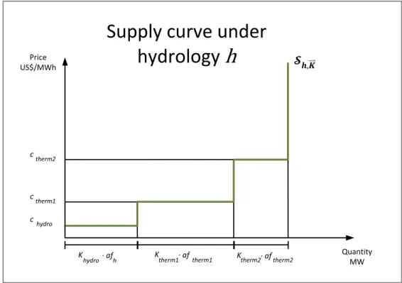
(18) 8. maximum output power for a thermal technology is constrained to its installed capacity multiplied by its availability factor. Supply is modeled in the short run by a supply curve4. For a given installed capacity ⃑⃑⃑ , defined over .. ⃑⃑. (. , there is one short run supply curve. ⃑⃑. for every. represents the set of combinations of production and price levels. ) at which producers are willing to deliver under the assumption of a. perfect competitive market. Figure 1 shows an example of a supply curve for a given ( ⃑⃑⃑ ).. Supply curve under hydrology h. Price US$/MWh. ,⃑⃑⃑. c therm2. c therm1 c. hydro. K. hydro. ∙ af. h. K. ∙ af. therm1. therm1. Ktherm2∙ af therm2. Quantity MW. Figure 1. Example of a short run supply curve for a hydrological scenario . Technologies are ordered in strict merit order. As we assume a perfect competitive market, the price of the short run supply curve will be equal to the marginal cost of 4. We formulate it as a curve instead of a function, because it may have completely horizontal portions, for example when a technology has a constant marginal cost; and there also exist completely vertical portions of the curve, for example when there’s no more available capacity..

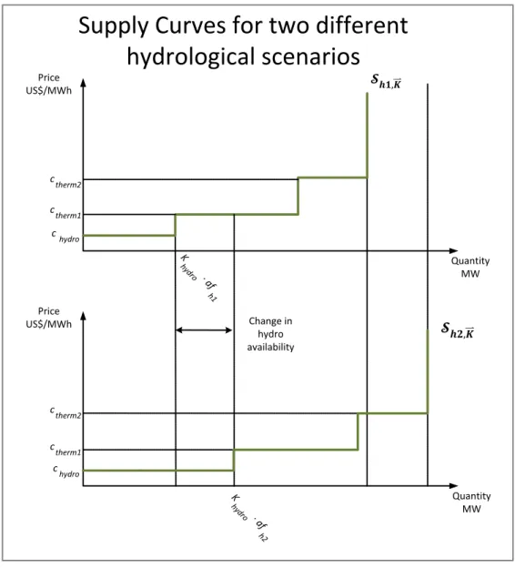
(19) 9. production of a given operating technology until there’s no more available capacity of that technology for a further increase of production. At that point, the supply curve turns into a vertical line until the price reaches the marginal cost of production of the next technology; or keeps vertical to. if it is the most. expensive technology in the system, and there is no more idle capacity for a further increase in production. Figure 2 shows how the short run supply curve changes form one hydrological scenario to another..

(20) 10. Supply Curves for two different hydrological scenarios Price US$/MWh. 𝟏,⃑⃑⃑. c therm2 c therm1 c hydro K. Quantity MW. hy. ∙a. o dr. f h1. Price US$/MWh. Change in hydro availability. 𝟐,⃑⃑⃑. c therm2 c therm1 c hydro K. Quantity MW. hy. ∙a. o dr. f h2. Figure 2. Comparison of short run supply curves for two hydrological scenarios. 2.4. Price Structures A price structure is defined as a set of exogenous constrains that prices must fulfill. In our model, we identify two price structures, one that rules the prices perceived by suppliers – namely supply price structure or wholesale price structure –, and another that defines the prices charged to final customers – namely demand.

(21) 11. price structure or retail price structure –. Typically, in a reformed electric system, there is a competitive hourly wholesale market, and some other kind of pricing structure for retail sales, such as a flat rate tariff. The supply price structure is defined as a set of restrictions defined over. . This price structure is imposed to the prices seen by generators. . Similarly, the demand price structure is defined as restrictions defined over prices seen by customers. , a set of .. For example, a flat rate tariff is a demand price structure in which prices are the same for every system’s state:. ̅. 2.4. 2.5. Short run equilibrium As there is a short run supply curve function. (. ) for every element of. for every element of. ⃑⃑. for every element of. and a demand. , a short run equilibrium may be defined. . Therefore, the model must solve. short run equilibriums. Given a capacity vector ⃑⃑ , the first short run equilibrium condition is defined as price structures system’s state. such that generation equals consumption for every :.

(22) 12. 2.5. It must be pointed out, that this equilibrium condition (2.5) acts over prices through the demand function and the supply curve respectively. Therefore, prices must be such that produced quantity is equal to demanded quantity state by state, subject to demand and supply curves. As prices seen by customers and suppliers are not necessarily equal, short run equilibrium is characterized by two points: ( (. ) for generators for every system’s state. ) for customers, and .. The second short run equilibrium condition is that there is zero expected profit for retailers. This implies that the expected amount of money raised from charges to customers must be equal to the expected money generators receive. The revenues of generators (or costs of retailer) may be expressed as the incomes from energy sales and additionally, as in some markets, the price structure might also include an income in the way of a capacity payment, which is represented by in the following expression:. ∑ ∑∑. 2.6. If there’s no capacity payment in the price structure under study, simply. .. The money raised from customers (or revenues of retailer) might be formulated as:. ∑. ∑. 2.7.

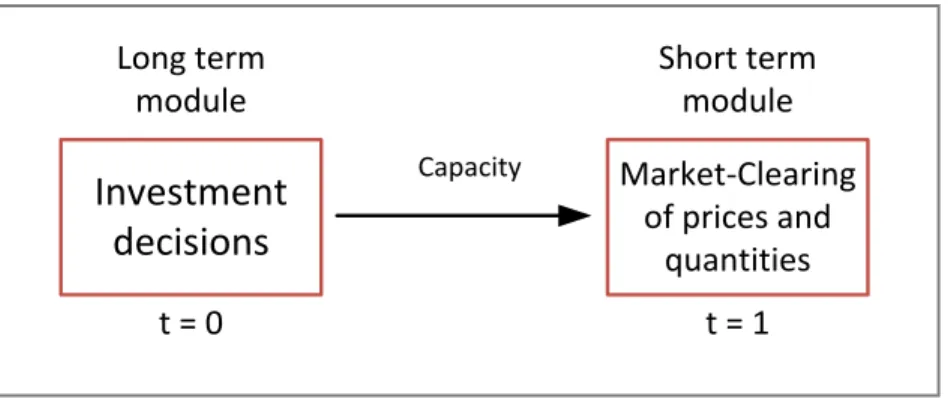
(23) 13. Then, the second short run equilibrium condition is defined, for a given capacity vector ⃑⃑⃑ , as price structures. such that retailers get zero expected. profit5:. ∑. ∑(. ). 2.8. Conditions expressed in equations 2.5 and 2.8 define the complete set of short run equilibriums for given price structures. , and for a given investment. decision ⃑⃑ . It must be noted that these equations impose a restriction to the space of price structures. Price structures are defined as “valid” if they satisfy equations 2.5 and 2.8, having as an outcome a unique pair of production and prices – (. ) and (. ) – for every. .. 2.6. Long run equilibrium The model developed is represented as a two stage game (see Figure 3). In the first stage, investment decisions are taken among the different available generation technologies. This is called the long run module. In the second stage, the short run market equilibrium is computed for every system’s sate (as described in previous section) given the investment decisions taken in the first stage. This is the short run module. The model seeks the equilibrium between long and short term, and finds out the complete equilibrium of the market (when both short and long term are in equilibrium).. 5. Note that this restriction imposes a risk distribution between agents..

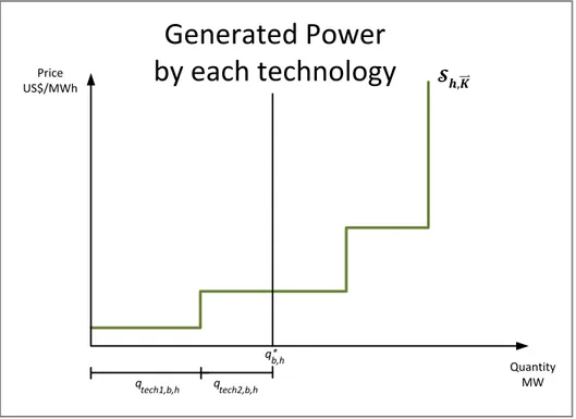
(24) 14. Long term module. Investment decisions. Short term module Capacity. t=0. Market-Clearing of prices and quantities t=1. Figure 3. Interaction between short and long term modules. Under the assumption of competitive market and free entry, every available technology must meet a zero expected Net Present Value (NPV) condition in the long run equilibrium. For describing the long run equilibrium, a further definition needs to be made. Let be the generated energy by technology. in system’s state. . The. amount of energy generated by each technology depends directly by the dispatch merit as shown in Figure 4..

(25) 15. Price US$/MWh. Generated Power by each technology. ,⃑⃑⃑. * qb,h. qtech1,b,h. qtech2,b,h. Quantity MW. Figure 4. Example of generated power by each technology for a given short run equilibrium’s total generated quantity . Long run equilibrium can be defined as a capacity vector ⃑⃑⃑ structures. and pricing. which satisfy short run equilibrium conditions 2.5 and 2.8,. such that generators’ expected incomes are equal to their expected costs:. ∑. ∑(. ). 2.9.

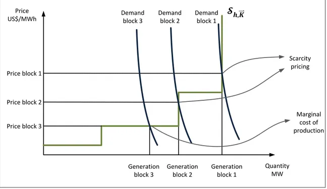
(26) 16. 3.. STUDY CASES. In this section we describe the particular cases that we study and simulate. 3.1. Dynamic pricing (DP) In this case, the supply price structure is assumed as a competitive wholesale market with no price restriction whatsoever. Regarding the demand price structure, under dynamic pricing it is assumed that customers are exposed directly to competitive wholesale prices. This means that customers see the same prices as generators. Equation 3.1 shows this relation:. 3.1. As the equilibrium also must satisfy the general equilibrium condition expressed in equation 2.5, the short run equilibrium condition can be expressed directly as the intersection between the demand and supply curves for each demand block and hydrological scenario. This also satisfies the short run equilibrium condition of retail’s zero profit (equation 2.8), because the price and quantity that generators and consumers see are the same at every moment. Therefore, is direct that revenues of generators are equal to the payments made by consumers for every state. .. As shown in Figure 5, in an equilibrium given directly by the intersection of supply and demand curve, as it takes place with dynamic pricing, the market clearing process can happen in two ways. It might be “supply side”, at marginal production cost, or “demand side”, at scarcity prices. This is a relevant aspect, as it enables the market to achieve the long run equilibrium. The process of scarcity pricing is what allows the price of energy to rise even over the highest marginal.

(27) 17. production cost so that generators can obtain sufficient revenues to cover their fixed investment costs. In such a market there’s no need of a capacity payment.. Price US$/MWh. Demand block 3. Demand block 2. ,⃑⃑⃑. Demand block 1. Scarcity pricing Price block 1. Price block 2 Marginal cost of production. Price block 3. Generation block 3. Generation block 2. Generation block 1. Quantity MW. Figure 5. Short run equilibrium. For each hydrological scenario it is possible to calculate the incomes and costs of generators, with which the expected NPV can be determined:. ∑. ∑(. ). 3.2. As was stated before, the long term equilibrium condition is that the expected NPV is zero for all technologies. This means to find an optimal investment decision ⃑⃑⃑ , where a deviation in one unit of capacity for any technology would mean that condition 2.9 is no longer fulfilled. As studied by peak load pricing theory (Borenstein & Holland, 2005; Chao, 2011) this point ⃑⃑. is unique and for this. particular pricing structure achieves the minimum supply cost..

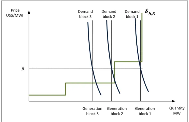
(28) 18. 3.2. Flat rate tariff (FR) In this case it is assumed that all customers are under a flat rate tariff. This means that all customers pay a fixed value for their energy which changes neither across hours nor with hydrology. The retail price structure can be formalized as:. ̅. 3.3. Where ̅ is the flat rate tariff. Demanded quantity is determined directly for every system’s state by replacing the flat rate tariff in equation 2.2 (demand function):. ̅. 3.4. Graphically, this can be seen as the intersection of demand curves of each block with the flat rate tariff as shown in Figure 6..

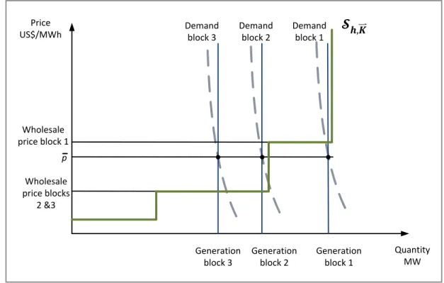
(29) 19. Price US$/MWh. Demand block 3. Demand block 2. Demand block 1. ,⃑⃑⃑. p. Generation block 3. Generation block 2. Generation block 1. Quantity MW. Figure 6. Short run equilibrium under flat rate tariff. It must be noted that as ̅ doesn’t change with the hydrological scenario, the total demanded quantity for a given demand block is the same for all hydrological scenarios. ̅. .. In the wholesale market, a flat rate price structure has the effect of making demand completely inelastic to changes in wholesale market prices. This is because customers don’t see wholesale prices. Figure 7 shows how the short run equilibrium happens under such price structure. Instead of the intersection between demand and supply curve, in this case, the supply curve intersects with completely inelastic demand given by the demanded quantity under the flat rate tariff. This formulation satisfies the short run equilibrium condition expressed in equation 2.5 as demanded quantity is equal to generated quantity for every system’s state..

(30) 20. Price US$/MWh. Demand block 3. Demand block 2. Demand block 1. ,⃑⃑⃑. Wholesale price block 1 p Wholesale price blocks 2 &3. Generation block 3. Generation block 2. Generation block 1. Quantity MW. Figure 7. Wholesale prices under flat rate tariff. This condition presents a problem that needs an additional rule to be defined for the wholesale price structure. When the inelastic version of the demand curve intersects with a vertical portion of the supply curve, i.e. in scarcity situations, price cannot be defined by a single point. In a real market this is typically observed by extremely high and volatile prices. In this situations is uncertain how a market may clear (if it manages to clear at all), and this is generally solved by the introductions of price caps. The additional rule we introduce is a price cap and we assume it equal to the variable cost of the most expensive technology6. As a consequence, under a flat rate retail price structure, it’s not possible for scarcity prices to emerge; therefore generators can’t get sufficient revenues to cover their fixed investment costs. As discussed in Borenstein (2005) in a market. 6. If a higher price cap is chosen, then a lower capacity payment is needed as generators perceive more incomes from spot market. The effects these different combinations of price cap / capacity payment may have on market equilibrium are not subject of study of this work..

(31) 21. of such characteristics, a capacity mechanism is necessary, in order that the market can always achieve a “supply side” clearing. We assume a fixed by regulator price. of capacity equal to the peaking. technology annuity divided by its availability factor7.. 3.5. Also, following the market structure described in Bernstein (1988)8, we assume that the payments that generators receive are proportional to their “firm capacity” (nominal capacity adjusted by availability) and to the maximum system’s demand. As Bernstein (1988) shows, a capacity payment compelling those rules assures enough payments to generators to cover their investments. As summary, the capacity eligible for capacity payment is adjusted by two factors: -. For thermal technologies by the deterministic availability factor, and for hydro technology, by the driest hydrological scenario.. -. By the system’s maximum demanded quantity9.. In this way, the capacity payment perceived by generators is the following:. ⃑⃑ ̅. 7. ⃑⃑ ̅. 3.6. In the Chilean market the capacity price is defined in this way, and is the cost of giving an additional MW in the peak 8 Which is the market structure applied in Chile. 9 This adjustment is required for the existence of long term equilibrium, otherwise there would be no limit to investment in peaking technology due to the fact that the capacity mechanism would always pay the exact value of the investment annuity..

(32) 22. Where : Installed capacity in technology. [MW].. : Capacity payment perceived by technology : The deterministic availability factor driest availability factor. [US$].. for thermal technologies and the. for hydro technology.. ⃑⃑ ̅ : Correction factor according to system’s maximum demand (see equation 3.7). : Capacity price [US$/MW/year]. ⃑⃑ ̅ is calculated through the following expression:. ⃑⃑ ̅. Where. ̅. 3.7. ∑. ̅ is the system’s maximum demanded power. [. ]. Now, with supply and demand pricing structures fully defined, it is possible to formulate the equilibrium condition of retail’s zero profit. Generators revenues are given by the following expression:. ∑ ∑∑. 3.8.

(33) 23. While payments made by customers are equal to consumption multiplied by the flat rate tariff10:. ∑ ̅. 3.9. Therefore, the equilibrium condition is satisfied for a ̅ such that:. ∑ ∑∑. ∑ ̅. 3.10. From 3.10, ̅ can be expressed as the load weighted average of wholesale prices plus an uplift for financing the capacity mechanism of the wholesale price structure:. ̅. ∑. ∑. ∑ ∑. 3.11. From equation 3.11, it can be seen the recursive characteristic of definition ̅ ; because both, quantity and wholesale prices depend of the flat rate tariff though demand function. Given that there is no analytic solution to equation 3.11, a computational iterative process based on Newton’s algorithm is used to find ̅ . For the long run equilibrium, in this case, generators have the additional revenues from the capacity mechanism. The expected NPV of each technology can be calculated as:. ∑ ∑(. 10. ). Note that this expression doesn’t depend of the hydrological scenario.. 3.12.

(34) 24. The long run equilibrium is found for a ⃑⃑. that makes equation 3.12 equals zero. for every available generation technology. 3.3. Chilean tariff In this section a “Chilean like” tariff is described and its equilibrium is characterized. In Chile, most consumption pays a flat rate “energy tariff” and a capacity charge during administratively set peak hours. From the point of view of Chilean consumers, the capacity charge might be formulated as an uplift in energy price during those hours defined as peak hours. In strict sense, in Chile customers pay for their maximum demanded quantity coincident with system’s maximum demanded quantity during peak hours. As no customer knows ex-ante when the maximum demand might happen, it seems a reasonable approximation to model the capacity charge as an uplift in energy price that represents the over cost that customers are exposed during peak hours. As a result, consumers perceive two different prices depending on if it a “peak”11 or “off peak” hour (see Figure 8). As these prices are defined ex-ante, they are the same for every hydrological scenario. For off peak hours, price is defined as:. ̅. 3.13. While during peak hours, the price is the flat rate plus an uplift:. 11. In the simulation, in order to avoid peak reversal, a different number of demand blocks are predefined as “peak hours” depending on demand elasticity simulated. For details see section 4.3..

(35) 25. ̅. 3.14. As a summary, this retail price structure is composed of two periods of time with different ex-ante fixed prices that don’t change with the hydrological scenario.. Price duration curve. Price US$/MWh Peak Price. Off peak Price. Peak Hours. Off peak Hours. Time Hours. Figure 8. Price duration curve for Chilean like tariff. The wholesale market price structure is defined the same as for the completely flat rate tariff. This means, that there’s a capacity payment and a wholesale energy market. In the Chilean tariff, the capacity payment is adjusted to the maximum demanded quantity during peak hours, because only in those hours customers pay for capacity. Higher price during peak hours have as result a reduction of consumption during those hours. As demand’s elasticity is increased, this effect is high enough that might happen that off peak maximum demanded quantity is higher than peak maximum demand quantity. This phenomenon is known as peak reversal and its.

(36) 26. consequence is that the capacity mechanism is not able to finance enough capacity for the system’s global maximum demanded quantity. To avoid this problem, for the simulations, the amount of demand blocks defined as peak hours are adjusted correspondingly to the demand’s elasticity. A capacity charge placed during more hours implies that a lower uplift is needed; therefore, the chance of having a peak reversal is reduced. The short run equilibrium for this kind of tariff is very similar to a completely flat rate tariff’s equilibrium. The tariff level defines quantity through demand function, while quantity defines wholesale prices through supply function. In the case of the retailer zero profit condition, there exists a difference with the completely flat rate tariff. In this case, there can be formulated two separate components: the uplift, that finances the capacity mechanism, and the off peak tariff that finances generators’ revenues from sales of energy in the spot market. Equation 3.15 shows the total revenues from retail sales.. ∑. ̅. ∑. ̅. 3.15. This can also be expressed as:. ∑. ∑ ̅. 3.16. The price structure studied imposes that the first term must be equal to the revenues that generators perceive by the capacity mechanism:.

(37) 27. ∑. ∑. 3.17. So in an equilibrium tariff, the rest of generators’ revenues must be covered by ̅ :. ∑ ̅. ∑ ∑∑. 3.18. This can be expressed as:. ̅. ∑. ∑. ∑ ∑. 3.19. So, for a Chilean like tariff, the “regular” tariff ̅ is equal to the load weighted average of the wholesale prices, while the uplift – as the regulatory construction of this price structure mandates – covers only the revenues associated with the capacity mechanism. For this tariff, the long run equilibrium keeps the same structure than previous case..

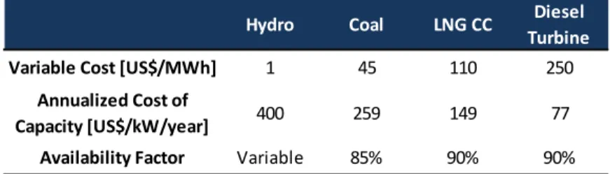
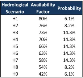
(38) 28. 4.. SIMULATIONS’ INPUT DATA 4.1. Technologies For the simulations we consider four different technologies available in the model; hydroelectricity, coal, LNG and diesel. As was stated in section 2.3, each technology is characterized by its variable operating cost, its annual investment cost12 and its availability. The technologies’ data is presented in Table 1. These numbers are intended to reflect typical generation costs in the Chilean SIC. Table 1. Technologies’ characteristics13.. Hydro. Coal. LNG CC. Diesel Turbine. Variable Cost [US$/MWh]. 1. 45. 110. 250. Annualized Cost of Capacity [US$/kW/year]. 400. 259. 149. 77. Availability Factor. Variable. 85%. 90%. 90%. 4.2. Hydroelectric availability The simulation is realized for nine non-equiprobable hydrological scenarios. These scenarios are constructed from 49 years (1960 to 2008) of hydrological Chilean statistics. Each hydrological scenario is defined by its probability and the availability of hydroelectric power plants, as shown in Table 2.. 12. A discount rate of 10% is assumed. Hydro investment cost is set artificially high in order that results reflect roughly present hydroelectric participation in SIC. This high value would be representing the shadow price of hydroelectricity given environmental restrictions, political uncertainty, public opposition to hydroelectric projects and water rights concentration, among other issues. 13.

(39) 29. Table 2. Availability and probability of hydrological scenarios. Source: Constructed from October 2011 node price calculation by Comisión Nacional de Energía, Chile14. Hydrological Availability Probability Scenario Factor H1 80% 6.1% H2 76% 8.2% H3 73% 14.3% H4 70% 14.3% H5 66% 14.3% H6 63% 14.3% H7 58% 14.3% H8 54% 8.2% H9 42% 6.1%. 4.3. Demand’s parameters As can be seen in equation 3.4, one of the parameters that has to be estimated is the demand’s elasticity. There are many studies of the elasticity of the demand for electricity. They show that demand responds differently depending on the time frame, i.e. depending if it is in the short run or in the long run. Benavente et al. (2005) estimate Chilean household’s demand elasticity between -0.055 in one month and -0.39 in the long run. For the purpose of this work, the relevant elasticity would be some medium-run elasticity, as prices generally follow a periodic profile or seasonal pattern. Also the change of general price levels, depending on the hydro availability, fits best under a medium-run elasticity as hydroelectric scenarios change on a yearly basis. In practice, short run elasticity would also be relevant, as there are situations like the stochastic behavior of demand with changes that manifest from hour to hour, or the uncertainty over outages that may suddenly happen in power plants or transmission lines. To 14. The hydrological scenarios are constructed from the hydrological statistics of run-of-river centrals. The statistics are grouped into 10 synthetic scenarios, which are shown in the table..

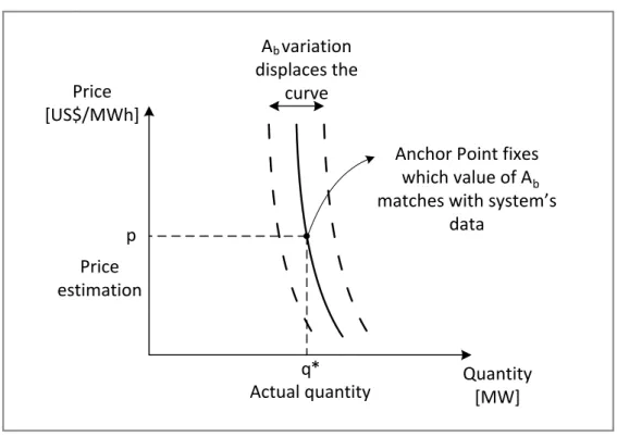
(40) 30. further increase the discussion, even long run elasticity would be relevant, as consumers adapt their facilities, industries, houses, appliances or behavior to the expected price profile. To avoid getting stuck in this discussion a wide range of elasticities is modeled going from -0.05 (short run) to -0.4 (long run). This range is consistent with ranges proposed by several studies, as reported in a summary table in Galetovic & Muñoz (2011). The following Table 3 shows the number and duration of blocks used to represent the demand in the simulations. The 500 hours of highest demand were represented by one hour blocks to have a better view of the phenomena that happen in peak hours. Table 3. Blocks used to represent the demand curve Duration [hours] Number of Blocks. 1 500. 236 35. Following Borenstein (2005), the demand function of every block is determined by an anchor point that allows calculating the. parameter of equation 2.2. The. anchor point of every hour is defined by the actual power demanded during that hour taken from SIC’s data, and by an estimation of the average price charged to customers during that period15. With the anchor point defined, it is possible to calculate the. parameter for every hour, thus recovering the shape of the load. distribution. Figure 9 shows how with an estimation of price and quantity, the demand function can be completely defined. Elasticity of -0.1 is considered as the base case to obtain hourly “anchor points”. For different values of demand’s price elasticity, the parameter 15. is changed in. For hours defined as “peak hours” by Chilean regulation, and therefore subject to a capacity charge, an uplift over energy price was assumed equal to capacity price divided by the amount of “peak hours”..

(41) 31. such a way, that under flat rate tariff the result is the same, regardless the elasticity considered.. Price [US$/MWh]. Ab variation displaces the curve Anchor Point fixes which value of Ab matches with system’s data. p Price estimation. q* Actual quantity. Quantity [MW]. Figure 9. Fixing demand curve by an anchor point. Regarding the prices utilized for the anchor points, it must be pointed out that there is no big error in using a rough estimation of an aggregated price. As can be seen in Figure 10, for the low elasticities modeled, a “big” mistake in the price of the anchor point would not cause a significant mistake in the estimation of the demand curve. As is discussed in Borenstein (2005), the relevant factor for characterize the long run equilibrium is not the actual demand hour by hour, but the shape of the load duration curve. With a rough price estimate, given the range of elasticities taken into account, it is possible to obtain a reasonable accurate representation of the shape of load duration curve. For this exercise, we use the.

(42) 32. SIC’s mean market price16 published by the Comisión Nacional de Energia, which is a moving average of power contracts’ prices through 4 months. Price [US$/MWh]. Ab variation. Anchor Point. p Price Estimation Actual price. p*. q* Actual quantity. Quantity [MW]. Figure 10. Anchor point with a mistaken price estimation. In the case of the Chilean tariff, for avoiding peak reversals, the following demand blocks are considered as “peak hours”17: Table 4. Number of hours and corresponding demand blocks defined as “peak hours”. Elasticity "Peak Hours" "Peak Blocks". 16. -0.05 736 501. -0.1 736 501. -0.2 1,444 504. -0.3 1,916 506. -0.4 2,388 508. Precio Medio de Mercado (PMM) Of a total of 535 blocks that represents the load duration curve, where the first 500 are 1 hour blocks, and the last 35 of 236 hours. 17.

(43) 33. 4.4. Solution algorithm for the simulations The equilibrium problem is solved by a computational iterative search using bisection, secant and Newton’s method, until all equilibrium conditions are satisfied. A basic flowchart describing the iteration process is shown below:. Change of investment in technology tech. Short run equilibrium for every system’s state. NO. Expected present value = 0?. YES. Next technology. YES. Expected NPV of all technologies = 0?. NO. END. Figure 11. Computational iteration process. Basically, the solution algorithm works by finding the investment decision of equilibrium for a technology given the installed capacity in the other technologies. Then the process is repeated for the next technology, and so on, until the expected.

(44) 34. NPV is zero simultaneously for all technologies. At this point the long run equilibrium of the system is achieved. Also must be pointed out that every expression without an analytic solution were solved using the same algorithm (as for example equation 3.11)..

(45) 35. 5.. SIMULATIONS’ RESULTS AND ANALYSIS. In this section we compare results for the different pricing structures previously defined. First, a comparison between flat rate tariff and dynamic pricing is presented, and in second place, the results for the Chilean tariff are presented (also respect to a completely flat rate tariff). 5.1. Dynamic pricing vs. Flat rate tariff 5.1.1. Social Surplus The increase in social welfare caused by changing from a flat rate tariff (FR)18 to a dynamic pricing (DP) scheme is calculated. As the long run equilibrium condition is expected NPV equal zero, there’s no producer surplus for neither case. As a consequence only changes in the consumer surplus (. ). contribute to the total. increase of social welfare. With the demand function given by equation 2.2, the effect in social welfare of introducing dynamic pricing is given for each demand block and hydrological scenario by the integral between the price paid by customers under one price structure and another (graphically in Figure 12 and analytically in equation 5.1).. 18. From now on, when we say “Flat Rate Tariff” (FR), we mean the flat rate tariff component plus a capacity component..

(46) 36. Price [US$/MWh] ΔCS b,h. p FR. DP pb,h. Quantity [MW]. Figure 12. Graphic representation of consumer surplus. ̅. ∫. Where ̅. ( ̅. (. ). ). 5.1. denotes de price paid by customers under dynamic pricing (DP) and. the price paid under a flat rate tariff (FR).. Then, the total expected consumer surplus is calculated by adding over all the system’s states:. ∑ ∑. (( ̅. ). (. ). ). 5.2. Table 5 presents the total supply cost and the increase of social surplus compared to the flat rate case for the five simulated elasticities. Gains go from 4% to 13% of the total cost of supply under flat rate regime..

(47) 37. Table 5. Annual cost of supply and social surplus (FR: Flat Rate tariff; DP: Dynamic Pricing). Values in million US$/year Elasticity -0.05 TOTAL OPERATION AND INVESTMENT COST FR Annual inv. & op. cost 3,639 DP Annual inv. & op. cost 3,507 Difference -132 Diff. as % of total FR supply cost -4%. -0.1. -0.2. -0.3. -0.4. 3,640 3,448 -192 -5%. 3,640 3,378 -262 -7%. 3,636 3,354 -282 -8%. 3,639 3,357 -282 -8%. TOTAL EXPECTED CONSUMER SURPLUS E{ΔCS} 139 E{ΔCS} as % of total FR supply cost 3.8%. 211 5.8%. 324 8.9%. 405 11.1%. 469 12.9%. Social gains are due to the fact that under dynamic prices every market agent is exposed to efficient price signals that accomplish to establish an effective communication between demand and producers. With DP, unlike with FR, producers know the willingness to pay of consumers in every moment, and with that information discern which investment and production decisions are the most valuable. A correct price signal stimulates customers to adapt their consumption to supply conditions, and gives producers the incentives to adequate their investments and production to demand’s needs. In this way, an efficient resource allocation is achieved. Also, as expected, the benefit of dynamic pricing grows as the demand becomes more elastic. A greater elasticity implies that it is “cheaper” for the demand side to respond. As previously suggested, a flat rate tariff turns the demand into a completely inelastic function, and thus, a greater opportunity of efficiency is missed..

(48) 38. In the long run, as smart metering and control technologies are further developed and demand response becomes easier, it might be expected that demand shifts to a situation of increased demand elasticity. Having this in mind, benefits from dynamic pricing might be even larger than the ones reported on Table 5. Also, it must be pointed out that there is a large number of uncertainties and sources of variability that are not considered in this model, such as outages, short run weather stochastic behavior, long run uncertainty on demand’s growth rate, uncertainty in transmission investments, etc. All these kind of phenomena are likely to make dynamic pricing even more efficient if compared to a flat rate tariff. 5.1.2. Prices With dynamic prices there is a reduction of 9% to 12% of the mean price paid by customers (see Table 6). Table 6. Retail prices statistics over all system’s states. .. Expected Retail Price [US$/MWh] Elasticity Flat Rate Tariff Dynamic Pricing Difference. -0.05 86.1 78.6 -9%. -0.1 86.1 78.6 -9%. -0.2 86.1 77.9 -10%. -0.3 86.1 76.9 -11%. -0.4 86.1 76.1 -12%. Table 7 displays statistics of the wholesale prices under both kinds of price structures. It can be seen that as opposite to the retail market, the mean wholesale price under a flat rate regime is lower than under dynamic pricing. This is caused by the capacity mechanism, which as shown in section 5.1.3, stimulates the investment in additional capacity, which makes prices lower..

(49) 39. Table 7. Wholesale price statistics for DP and FR over all system’s states . Wholesale Prices [US$/MWh] Elasticity FLAT RATE TARIFF Mean Price Maximum Price Minimum Price Std. Dev.. -0.05. -0.1. -0.2. -0.3. -0.4. 68.7 250.0 1.0 52.0. 68.7 250.0 1.0 52.3. 68.7 250.0 1.0 52.0. 68.6 250.0 1.0 52.1. 68.7 250.0 1.0 52.0. DYNAMIC PRICING Mean Price 78.6 Maximum Price 9,854.1 Minimum Price 1.0 Std. Dev. 138.9. 78.6 2,787.6 4.6 107.4. 77.9 990.8 9.7 76.9. 76.9 580.5 12.7 59.3. 76.1 409.4 16.5 47.9. An also interesting result is how with increased elasticity, the spike prices under DP are reduced significantly from over 9,000 US$/MWh to almost 400 US$/MWh. Larger demand elasticity contributes to smooth down system’s volatility, result that can also be seen in the reduction of standard deviations (Table 7). Figure 13 shows the price probability distribution over all system’s states for dynamic pricing with a demand’s price elasticity of -0.1, and Figure 14 shows a zoom in on the price distribution for prices higher than 200 US$/MWh. From Figure 13 can be seen that prices approximately 75% of the time are under 100 US$/MWh, while Figure 14 shows that prices over 200 US$/MWh roughly occur 7% of time..

(50) 40. 0.70. 1 0.9 0.8 0.7 0.6 0.5 0.4 0.3 0.2 0.1 0. Probability. 0.60 0.50 0.40 0.30. 0.20 0.10 0.00. Cumulative Probability. Price Probability Distribution. DP elasticity -0.1. Price [US$/MWh]. Figure 13. Price distribution under dynamic pricing. As wholesale prices are equal to retail prices, this figure represents distribution of both prices.. Probability. 0.04. 0.08 0.07 0.06 0.05 0.04 0.03 0.02 0.01 0.00. 0.03 0.02 0.01. 0.00. Price [US$/MWh]. Figure 14. Peak price distribution under dynamic pricing.. Cumulative Probability. Peak Price Probability Distribution. DP elasticity -0.1.

(51) 41. On the other hand, Figure 15 shows the wholesale price distribution over. .. As was explained before, for a market with this kind of price structure there can’t happen a scarcity pricing phenomena, so possible prices are only equal to technologies’ marginal costs of production. .. 0.70 0.60 0.50 0.40 0.30 0.20 0.10 0.00. 1 0.8 0.6 0.4. 0.2 0. Cumulative Probability. Probability. Wholesale Price Probability Distribution. FR elasticity -0.1. Price [US$/MWh]. Figure 15. Wholesale price distribution under flat rate tariff. 5.1.3. Capacity composition The following table compares the total installed capacity under each price regime:.

(52) 42. Table 8. Total capacity and expected generation for simulated cases (FR: Flat Rate tariff; DP: Dynamic Pricing)19. Elasticity FR Total Capacity [MW] DP Total Capacity [MW] Difference. -0.05 10,066 8,705 -14%. -0.1 10,066 8,261 -18%. -0.2 10,066 8,032 -20%. -0.3 10,066 8,143 -19%. -0.4 10,066 8,274 -18%. FR Expe. Generation [GWh] DP Expe. Generation [GWh] Difference. 42,262 42,997 2%. 42,262 43,679 3%. 42,266 45,019 7%. 42,263 46,224 9%. 42,259 47,213 12%. Table 8 shows the effect that dynamic prices have on investment decisions. As can be observed, there is a large reduction on installed capacity of up to 20% for a -0.2 elasticity. Also, it can be seen an increase in generated energy. This reinforces the idea of greater efficiency in resource allocation, as there is a more efficient and intensive use of sunk capital goods. The impact of dynamic pricing may also be appreciated in the resulting technological mix of the long run equilibrium. Figure 16 shows the system’s technological composition for the different simulated elasticities.. 19. The difference in installed capacity is smaller for higher elasticities due to the fact that for DP, under higher elasticities, hydroelectricity has a higher participation. As hydroelectricity has a lower plant factor than thermal technologies, the total installed capacity increases for the highest elasticities..

(53) 43. Capacity 12,000. 10,000 MW. 8,000. 6,000. Diesel. 4,000. LNG. 2,000. Coal. 0. Hydro DP. Flat rate. Elasticity 0.05. DP. Flat rate. Elasticity 0.1. DP. Flat rate. Elasticity 0.2. DP. Flat rate. Elasticity 0.3. DP. Flat rate. Elasticity 0.4. Figure 16. Resulting capacity of simulations. It can be seen that there is a significant change in the system’s composition. Diesel, the peaking technology, almost disappears, while dynamic pricing promotes the investment in base-load technologies, in this case, hydroelectricity. With dynamic pricing, hydroelectricity participation as percentage of total installed capacity goes from 62% with an elasticity of -0.05, to 100% with an elasticity of -0.4. With dynamic pricing, the market is not only cleared from the “supply side”, but now demand also contributes. This is an important issue when dealing with a resource with stochastic availability like water. 5.1.4. Load duration curve Figure 17 shows an important effect in consumption decisions. There is an important adaptation of the load duration curve to the hydrological conditions..

(54) 44. This result in a better use of the hydro resource as demands responds to its availability.. Load duration curve under different scenarios for -0.1 demand elasticity 7,000 Flat rate tariff 6,500 Dynamic Pricing, wetter hyd. scenario. Demand [MW]. 6,000. Dynamic Pricing, driest hyd. Scenario Dynamic Pricing, Expected result. 5,500. 5,000 4,500. 4,000 3,500 3,000 0. 730 1460 2190 2920 3650 4380 5110 5840 6570 7300 8030 8760 Hour. Figure 17. Load duration curve for flat rate tariff and dynamic pricing under the expected and most extreme hydrological scenarios (demand elasticity is 0.1)..

(55) 45. 5.2. Chilean vs. flat rate tariff In this section the simulations results for the Chilean tariff are presented. 5.2.1. Social Surplus The Chilean tariff scheme, of two predefined price blocks, only captures a rather small part of dynamic pricing efficiency. The increase in social surplus goes from 1% to 3% compared to a flat rate tariff regime as shown in Figure 18.. ΔCS as % of total supply cost respect flat rate tariff 14% 12% 10% 8% 6% 4% 2% 0% -0.05. -0.1. -0.2. -0.3. -0.4. Demand Elasticity Dynamic Pricing. Chilean Tariff. Figure 18. Dynamic pricing and Chilean tariff increase in social welfare respect flat rate tariff. Table 9 presents the total supply cost and the increase of social surplus for the five simulated elasticities..

(56) 46. Table 9. Annual cost of supply and social surplus (FR: Flat Rate tariff; CT: Chilean Tariff). Values in million US$/year Elasticity -0.05 TOTAL OPERATION AND INVESTMENT COST FR Annual inv. & op. cost 3,639 CT Annual inv. & op. cost 3,621 Difference -18 Diff. as % of total FR supply cost 0%. -0.1. -0.2. -0.3. -0.4. 3,640 3,594 -46 -1%. 3,640 3,588 -51 -1%. 3,636 3,589 -47 -1%. 3,639 3,591 -47 -1%. TOTAL EXPECTED CONSUMER SURPLUS E{ΔCS} 25 E{ΔCS} as % of total FR supply cost 0.7%. 46 1.3%. 59 1.6%. 69 1.9%. 78 2.1%. Effects are not as large as under dynamic pricing because a Chilean like tariff takes into account, and in a very limited extent, only one dimension of system’s states: the variation of demand along the load duration curve, but it misses to incorporate the supply’s stochastic availability influenced by hydro uncertainty. This translate in a price structure almost as rigid as a flat rate tariff, as it cannot give the correct signals to market agents to adapt their decisions to current market conditions. Prices can’t go further up when there is a scarcity situation, neither further down when there’s abundance. As a result, the efficiency gains are narrowed down, and the only benefits come from the fact that price is higher during “peak hours”. This has two effects. First, there is a reduction in peak demand which overcomes with a reduction in investment in peaking technology (Figure 20); and second, the tariff for non peak hours is slightly lower than under a completely flat rate regime. This is because off peak hours now don’t include a component of price for financing the capacity payment mechanism. The two effects act combined flattening down the load duration curve (Figure 21)..

(57) 47. 5.2.2. Prices The following table shows the expected retail price for Chilean tariff compared with a flat rate tariff: Table 10. Retail prices statistics over all system’s states. .. Expected Retail Price [US$/MWh] Elasticity Flat Rate Tariff Chilean Tariff Difference. -0.05 86.1 83.4 -3%. -0.1 86.1 83.3 -3%. -0.2 86.1 83.1 -3%. -0.3 86.1 83.1 -3%. -0.4 86.1 83.1 -3%. Table 11 shows statistics of wholesale prices under Chilean tariff compared with wholesale prices under flat rate tariff. Table 11. Wholesale price statistic for CT and FR over all system’s states . Wholesale Prices [US$/MWh] Elasticity FLAT RATE TARIFF Mean Price Maximum Price Minimum Price Std. Dev.. -0.05. -0.1. -0.2. -0.3. -0.4. 68.7 250.0 1.0 52.0. 68.7 250.0 1.0 52.3. 68.7 250.0 1.0 52.0. 68.6 250.0 1.0 52.1. 68.7 250.0 1.0 52.0. CHILEAN TARIFF Mean Price Maximum Price Minimum Price Std. Dev.. 69.0 250.0 1.0 52.0. 69.0 250.0 1.0 51.9. 69.0 250.0 1.0 51.9. 69.3 250.0 1.0 51.7. 69.5 250.0 1.0 51.5.

(58) 48. Finally, the wholesale price distribution under Chilean tariff is displayed in Figure 19. As with flat rate tariff, there is no scarcity pricing, so the only prices observed are technologies’ marginal costs of production.. 0.70 0.60 0.50 0.40 0.30 0.20 0.10 0.00. 1 0.8 0.6 0.4. 0.2 0. Cumulative Probability. Probability. Wholesale Price Probability Distribution. CT elasticity -0.1. Price [US$/MWh]. Figure 19. Wholesale price distribution under Chilean tariff. 5.2.3. Capacity composition With Chilean tariff the changes in system’s technological composition are not as dramatic as with dynamic pricing. Nevertheless, in Figure 20 it is observed that diesel technology installed capacity is reduced for higher elasticities. The rest of technologies remain practically unaltered with Chilean tariff respect to flat rate tariff. Only a slight increase in hydro capacity may be observed as elasticity is increased..

(59) 49. Capacity 12,000. 10,000 MW. 8,000. 6,000. Diesel. 4,000. LNG. 2,000. Coal. 0. Hydro CT. Flat rate. Elasticity 0.05. CT. Flat rate. Elasticity 0.1. CT. Flat rate. Elasticity 0.2. CT. Flat rate. Elasticity 0.3. CT. Flat rate. Elasticity 0.4. Figure 20. Resulting capacity of simulations for Chilean Tariff. 5.2.4. Load duration curve Next figures show a comparison of the load duration curve, with a zoom in for 500 highest demanded quantity hours..

(60) 50. Load duration curve for -0.1 demand elasticity 7,000 Flat rate tariff. 6,500. Chilean Tariff. Demand [MW]. 6,000 5,500. 5,000 4,500. 4,000 3,500 3,000 0. 730 1460 2190 2920 3650 4380 5110 5840 6570 7300 8030 8760 Hour. Figure 21. Load duration curve for flat rate tariff and Chilean tariff (demand elasticity is -0.1)..

(61) 51. Peak Load duration curve for -0.1 demand elasticity 6,700. 6,500 Flat rate tariff. Demand [MW]. 6,300. Chilean Tariff. 6,100. 5,900. 5,700. 5,500 0. 100. 200. 300. 400. Hour. Figure 22. Load duration curve for 500 highest demanded quantity hours (demand elasticity is -0.1).. 500.

(62) 52. 6.. CONCLUSIONS. In this work we develop a long run equilibrium model of an electric power system, i.e. and investment and operation model, that consider a matrix of system’s states that represents the different demand levels that exist along the load duration curve and the uncertainty source given by the stochastic availability of water. The model incorporates in an explicit way the interaction between wholesale and retail markets of electric energy and we study how the framework given by different price structures affects the transmission of market conditions between producers and final consumers, and thereby, affecting the system’s long run equilibrium. Also, we assess the magnitude of this phenomenon by performing simulations of market outcome with real Chilean SIC data. We show how a retail flat tariff leads to an unresponsive demand seen from the wholesale market. This distorted price signal alters customers’ efficient consumption decisions, which by the way, distorts investments. As the results of our simulations show, this has a significant impact in market efficiency, with a flat tariff, the prices are distorted and neither demand nor supply receives the most efficient price signals, with the results of a less intensive use of sunken capital goods and with more investment in peaking technology to supply a steeper load duration curve. Also, the inelasticity created by flat tariffs at retail level breaks the scarcity pricing process at wholesale markets, making for the need of an outside market mechanism in order that generators can have enough incomes to pay for investments. We show that with dynamic prices there’s no need for such a mechanism, as the scarcity situations give enough incomes to generators to pay for their investment costs. In the case of the Chilean tariff, we show that it only collects a small part of dynamic pricing efficiency. With the distinction between peak and off peak hours, it only partially incorporates variations along the dimension of the load duration curve of the system’s states matrix, but it fails to incorporate the hydrologic condition to the price signal..

(63) 53. Besides, our model may be easily extended to further include different sources of uncertainty. There is only needed to be added more dimensions to the states matrix. The model’s basics remain the same; the only difference is that the matrix is larger. A relevant factor that was not included in this study is the cost and characteristics of the technologies needed for a dynamic pricing scheme. Certainly, nowadays the level of penetration of these technologies represents a barrier to the introduction of dynamic prices, but as in the future the technologies prices go down it may be expected to be easier for the introduction of dynamic prices..

(64) 54. REFERENCES Albadi, M.H., El-Saadany, E.F. (2007). Demand response in electricity markets: An overview. Power Engineering Society General Meeting, IEEE, 1-5. Allcott, H. (2011). Rethinking real-time electricity pricing. Resource and Energy Economics , 33 (4), 820-842. Benavente, J. M., Galetovic, A., Sanhueza, R., & Serra, P. (2005). Estimando la demanda residencial por electricidad en Chile: El consumo es sensible al precio. Cuadernos de Economía , 42, 31-61. Bernstein, S. (1988). Competition, marginal cost tariffs and spot pricing in the Chilean electric power sector. Energy Policy, 16 (4), 369-377. Boiteux, Marcel, (1949). Peak load pricing (translated). Journal of Business 33, 157179. Bompard, E., Ma, Y., Napoli, R., Abrate, G., & Ragazzi, E. (2007). The impacts of price responsiveness on strategic equilibrium in competitive electricity markets. International Journal of Electrical Power & Energy Systems , 29 (5), 397-407. Borenstein, S. (2005). The long-run effiency of real-time electricity pricing. The Energy Journal , 26 (3), 93-116. Borenstein, S., & Holland, S. P. (2005). On the efficiency of competitive electricity markets with time-invariant retail prices. The RAND Journal of Economics, 36 (3), 469493. Bushnell, J. (2010). Building blocks: Investment in renewable and non-renewable technologies. Berkeley, Energy Institute at Haas..

(65) 55. Caves, D., Eakin, K. & Faruqui, A. (2000). Mitigating price spikes in wholesale markets through market-based pricing in retail markets. The Electricity Journal, 13 (3), 13-23. Chao, H. (1983). Peak load pricing and capacity planning with demand and supply uncertainty. The Bell Journal of Economics , 14 (1), 179-190. Chao, H. (2011). Efficient pricing and investment in electricity markets with intermittent resources. Energy Policy , 39 (7), 3945-3953. Doorman, G. L. (2000). Peaking capacity in restructured power systems. Doctoral thesis, Norwegian University of Science and Technology, Faculty of Electrical Engineering and Telecommunications. Doorman, G. L., & Botterud, A. (2008). Analysis of generation investment under different market designs. Power Systems, IEEE Transactions on, 23 (3), 859-867. Galetovic, A., Inostroza, J., & Muñoz, C. (2004). Gas y electricidad: ¿Qué hacer ahora?. Estudios Públicos, 96, 49-106. Galetovic, A., & Muñoz, C. (2011). Regulated electricity retailing in Chile. Energy Policy, 39, 6453-6465. Joskow, P. (2008). Capacity payments in imperfect electricity markets: Need and Design. Utilities Policy, 16 (3), 159-170. King, M. J., King, K., & Rosenzweig, M. B. (2007). Customer sovereignty: why customer choice trumps administrative capacity mechanisms. The Electricity Journal, 20 (1), 38-52. Montero, J. P., & Rudnick, H. (2001). Precios eléctricos flexibles. Cuadernos de Economía, 38, 91-109..