The Chandra COSMOS Legacy Survey: Energy Spectrum of the Cosmic X Ray Background and Constraints on Undetected Populations
8
0
0
Texto completo
(2) The Astrophysical Journal, 837:19 (8pp), 2017 March 1. Cappelluti et al.. 2016; Marchesi et al. 2016). Here, we present a novel precise measurement of the CXB, its unresolved fraction, and new constraints on the properties of z>6 black holes by using the Soltan argument.. allows us to obtain a measurement that is minimally affected by poor statistics or cosmic variance. We call the spectrum of all photons detected in the field of view (FOV) the CXB spectrum. However, to extract the unresolved CXB spectrum, we more carefully select the area used. Both Chandraʼs point-spread function (PSF) and effective area rapidly degrade with the offaxis angle. Consequently, at large off-axis angles, little to no usable area is left after excising detected sources. The Chandra PSF radius can be approximated with: r90 ~ 1″ + 10″(q 10¢)2 , where r90 is 90% Encircled Energy Radius and θ is the off-axis angle. Compromising the need to maximize photon count with the degradation of our observations with the off-axis angle, we found that the highest quality data can be obtained using the inner 5′ (θ=5′ r90 < 3. 5). To estimate the spectrum of the CXB after removing X-ray sources, we extracted the spectrum of the area remaining in the inner 5′ after removing the sources detected by Civano et al. (2016) using a 7″ radius region around each X-ray centroid. This radius corresponds to twice r90, which we consider large enough to neglect the flux of the PSF tails. Because of the mosaicking, with these choices we still cover most of the CCLS area and mask 3% of the pixels because of sources. This spectrum will be called uCXB (unresolved CXB). According to Figure 2 of Civano et al. (2016), and thanks to the tiling of the pointings, this radius safely includes almost the totality of the source fluxes even without limiting the investigation to the inner FOV. Note that the Chandra PSF is not circular but is elongated as a function of the azimuthal angle. Nevertheless, we were able to use circular apertures because the asymmetry of the PSF is washed out by the tiling of the survey, which averages over azimuthal angles. See, e.g., the treatment of PSF fitting in Cappelluti et al. (2016). To further probe the unknown discrete source CXB (hereafter nsCXB, non-source CXB), we extracted the spectrum of the area left after removing X-ray sources and HST-ACSdetected sources. These sources are so plentiful that using a 3 5 masking radius leaves little sky area to perform our measurement. For this reason, we used the approach of Hickox & Markevitch (2007) and limited the search to the inner 3 2 of axis of every pointing. We estimated that r90 < 2 2, and masked areas around each galaxy of the Scoville et al. (2007b) catalog. The choice of this radius is a trade-off, ensuring that a large fraction of the X-ray flux of the optical-/NIR-selected galaxies is removed and keeping the contamination from PSF tails under control (see below for the treatment of PSF tails). For each subsample, the net extracted counts are reported in Table 1. Remarkably, the CXB spectrum we derive contains ∼123,000 net counts. For each spectrum, we also computed the field-averaged Redistribution Matrix Functions (RMFs) and Ancillary Response Functions (ARF) using the CIAO tool specextract. Spectra were then co-added and response matrices averaged after weighting by the exposure time.. 2. Data set and Analysis The Chandra COSMOS-Legacy survey (CCLS; Elvis et al. 2009; Civano et al. 2016) is an X-ray Visionary Program that imaged the 2.2 deg2 COSMOS field (Scoville et al. 2007b) for a total of 4.6 Ms. The survey has an effective exposure of 160 ks over the central 1.5 deg2 and ∼80 ks elsewhere. A total of 4016 X-ray sources are detected down to flux limits of 2.2×10⁻¹⁶, 1.5×10⁻¹⁵, and 8.9×10⁻¹⁶ erg cm−2 s−1 in the [0.5–2], [2–10], and [0.5–10] keV energy bands, respectively. All the observations were performed in the VFAINT telemetry mode since it allows a lower instrumental background value. Here we briefly summarize our analysis, the details of which were mostly reported by Civano et al. (2016) and Puccetti et al. (2009). Level 1 data products were processed with the CIAO tool chandra_repro, retaining only valid event grades. Astrometry in each pointing was matched with the optical catalogs of Capak et al. (2007) and Ilbert et al. (2009). Particle background flares were removed using the deflare tool in compliance with the ACIS background analysis requirement after excising from the data set. In order to minimize uncertainties in modeling the quiescent particle background, we took special precautions to ensure that background flares were removed in a such a way that residuals from undetected faint flares were reduced. As shown in Hickox & Markevitch (2006), the [2.3–7] keV energy range is the most sensitive to particle background flares, and stowed-mode observations demonstrate that the [2.3–7] keV to [9.5–12] keV Hardness Ratio (HR) is constant. They also show that filtering the data for flares only in the [2.3–7] keV energy band results in missed periods of time during which the background has an anomalous HR. To account for this effect, we searched for flares not only in the [2.3–7] keV energy band, but also in the [9.5–12] and [0.3–3] keV bands. These “flared” time intervals were removed from the data (Cappelluti et al. 2009). With this procedure, we are confident that the remaining level of flaring is below 1%–2% (Hickox & Markevitch 2006), and therefore the amplitude of the quiescent particle background is subject to this level of systematic uncertainty. The Chandra X-ray Center (CXC) ACIS calibration team verified the validity of these assumptions, and no background anomalies have been reported as of 2016 May. X-ray source masking and/or stacking was performed to match the Civano et al. (2016) X-ray source catalog. For X-ray undetected galaxies, we used the Scoville et al. (2007a) catalog of ∼1 million detections by the Hubble Space Telescope down to mAB ~ 27–28 in the i-band. This enables a robust removal of faint X-ray undetected galaxies. Although Ilbert et al. (2009) and Laigle et al. (2016) assembled a catalog of ∼2 million galaxies, using these catalogs would have vastly reduced the area of our spectral extraction (see below) and made comparison with previous works more difficult. Moreover, for these last two catalogs, the coverage and sensitivities are uneven on the whole survey area.. 2.2. Background Treatment and Systematics In this analysis, we assumed that the only background components were the particle background and detector noise. ACIS-stowed observations were taken for about 1 Ms. In this mode, the detector records the particle background and detector noise. We searched the Calibration Data Base (CALDB) for observations taken during the period proximate to our observations, with the same chips and tailored ACIS background event files to each of our observations. For each pointing, we. 2.1. Spectral Extraction To obtain the spectrum of the full CXB, we use the entire ACIS-I area to maximize the collecting and survey area. This 2.
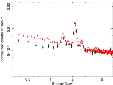
(3) The Astrophysical Journal, 837:19 (8pp), 2017 March 1. Cappelluti et al. Table 1 Spectral Analysis Results. Sample. Net Counts cts. CXB uCXB nsCXB. 123948 44642 11034. KPL ph cm−2 s−1 sr−1. Γ keV. kT1 keV. kT2. c 2 /dof. 10.91 0.16 (0.26 ) 4.18 0.26 (0.41) 1.37 0.30 (±0.45). 1.45 0.02 (0.03) 1.57 0.10 (0.16 ) 1.25 0.35 (0.62 ). +0.02 +0.03 0.270.02 (-0.04 ) 0.22 0.03 (0.06) 0.22 0.04 (0.05). 0.07 0.01 (0.02) +0.03 +0.04 0.080.01 (-0.03 ) La. 191.71/208 272.3/208 162/105. Note. In parentheses are the 90% confidence limits. a not required.. re-projected the stowed observation to the same observed wcs frame using the CIAO tool reproject_events; we verified that the stowed background events were calibrated with the same GAINFILE of our observations, and we ensured that the proper gain was used for all the “stowed” pointings. After these procedures we extracted the particle background spectra in the same areas described above (corresponding to the CXB, uCXB, and nsCXB regions). Hickox & Markevitch (2006, 2007) found that the spectral shape of the Chandra background is extremely stable in time and can be easily modeled for extended and diffuse emission like the CXB, by using ACIS observations taken in stowed mode. As mentioned above, the shape of the particle background spectrum is constant in time but its amplitude is not. We scale it by the ratio of the count rate in the [9.5–12] keV data (where no astrophysical events are recorded) to that in the stowed data. These ratios vary from 0.79–1.15. With this procedure, the systematic uncertainty on the background estimation is ∼2% (Hickox & Markevitch 2006). We averaged the background spectra of each pointing to take into account the different locations of the masked sources. We also subtracted out of time events (counts accumulated during readouts) that account for <1% of the total events. When using c 2 statistics, XSPEC is capable of handling systematic errors while fitting the data and adding them to the error budget. Therefore, by using the tool grppha, we included a 2% systematic in the stowed-background spectrum. Moreover, Leccardi & Molendi (2007) and Humphrey et al. (2009) report that the use of c 2 or CSTAT could produce biased results in the high-counts regime. According to Table 1 we expect a <2% bias in the fit results. We have factored an additional 2% systematic into our fits, for a total of ∼4% of systematics. Although an actual risk of underestimating the background does exist, at the 1%–2% level, this risk has been mitigated by treating the flares according to their hardness ratios. Without considering the 2% systematics, the fit does not change significantly. This is because the error budget is dominated by the intrinsic Poissonian error, associated with the stowed background, which has been estimated by accumulating onethird fewer photons than the real observation. This is clearly visible in Figure 1 where we compare the nsCXB spectrum and the PIB spectrum. There one can clearly note how the uncertainties are dominated by the statistical error on the PIB spectrum. Due to the uncertain background subtraction near instrumental emission lines, which may suffer from uncertainties of the order 5%–10% (Bartalucci et al. 2014), we limit our analysis to the [0.3–7] keV band and exclude the 2.0–2.4 keV energy range (which contains instrumental Au Mab lines).. Figure 1. Comparison of the nsCXB (red stars) before background subtraction and the PIB (black triangles). It is worth noting that the error bars of the PIB spectrum are much larger that those of the raw nsCXB spectrum.. 2.3. Spectral Fitting The observed spectra are shown in Figure 2. We fitted the observed X-ray spectra, grouped in bins of two channels, using XSPEC v12.9 (Arnaud 1996). In total the CXB and uCXB spectra have 213 spectral bins while the nsCXB has 98. The full [0.3–7] keV CXB consists of three principal components (Miyaji et al. 1998): (a) an extragalactic component produced by the integrated emission of resolved and unresolved discrete sources (AGNs, galaxies, and clusters), which we model as a power law (hereafter PL) times Galactic absorption with NH=2.0×1020 cm−2 (Dickey & Lockman 1990); for the absorption we used the tbabs model in XSPEC with crosssections form Verner et al. (1996) and abundances from Wilms et al. (2000). (b) A Galactic hot gas component with a temperature of the order kT∼0.15–0.25 keV, which we model using moderately absorbed (i.e., NH=N H,Gal ) emission from collisionally ionized diffuse gas (APEC, hereafter A1), known as the hard thermal component of the of the IGM whose temperature and intensity is a strong function of the galactic coordinates (see, e.g., Markevitch et al. 2003). (c) A lower temperature local bubble and/or geocorona, previously known as soft thermal CXB, modeled with an unabsorbed APEC hereafter A2). For these CXB components, we varied the following parameters: spectral Index Γ, PL normalization KPL, A1 and A2 normalizations, and temperature kT. NH was fixed for both PL and A1. Abundances were set to solar for both A1 and A2. However, we note that the temperatures and amplitudes of the soft components are slightly degenerate with the power-law 3.
(4) The Astrophysical Journal, 837:19 (8pp), 2017 March 1. Cappelluti et al.. into account because of the different sizes of the field of view employed for analyzing every subcomponent of the CXB.. 3. Results 3.1. Overall CXB Spectrum The CXB spectrum, the best-fit model, and its components are shown in Figure 2. The best-fit parameters are summarized in Table 1. The foreground local components have measured temperatures kT ~ 0.27 keV and kT ~ 0.07 keV , respectively. Both components are required at high significance level. Indeed, for our fit c 2 /dof=191.71/208 but if we remove the local bubble (soft thermal) component we obtain c 2 dof =231.62/ 208. We performed an f-test and, as a result, we found that the soft component is required at a 4.7σ level. If we remove the hard thermal component, the fit converges on a single power-law model but with c 2 dof 2. Above 2 keV, the emission can be totally ascribed to the extragalactic power-law component. The latter has a photon spectral index Γ=1.45±0.02, as in previous investigations (see, e.g., Gruber et al. 1999; Ajello et al. 2008) and a normalization KPL=10.91±0.16, consistent with previous Chandra (Hickox & Markevitch 2006), Swift (Ajello et al. 2008; Moretti et al. 2009), and ROSAT-ASCA results (Miyaji et al. 1998), yet lower than the early XMMNewton (De Luca & Molendi 2004) and higher than the ASCA and HEAO results (Gendreau et al. 1995; Gruber et al. 1999). This CXB unfolded spectrum is compared with these previous measurements in Figure 3. Due to the pencil beam nature of the survey, rare bright sources are not accounted for in our measurement. A precise estimate of their contribution is not possible with the data in hand, but using AGN population synthesis models (Gilli et al. 2007; Treister et al. 2009) we estimate that our measurement of the full CXB is underestimated by 3%. We rather not consider this to be a systematic error, but a limitation of our total CXB measurement. We have also measured the overall flux of the CXB in several energy bands and reported it in Table 2. The thermal contributions are dominant below 1 keV and account for about 23% of the overall [0.5–2] keV flux. The remainder of the flux can be ascribed to extragalactic emission, while above 2 keV most of the signal is extragalactic. The intensity of the Galactic components is in remarkable agreement with the micro-calorimeter measures of McCammon et al. (2002). 3.2. X-Ray Source Masked CXB Spectrum and Flux The uCXB, which is shown in Figure 2, has a slightly softer spectrum (G ~ 1.57) than the overall component (CXB), but still consistent with it. The Galactic foregrounds have, within the uncertainties, the same intensity and shape as the CXB. The uCXB spectrum is shown in Figure 5. Even in this case we obtain an excellent fit with three components with c 2 /dof=272.3/208. The slightly softer spectral slope is consistent with the observed higher fraction of Type I AGNs among the brightest sources. In Table 3 we show the fraction of resolved CXB as a function of energy. The removal of X-ray sources produces a drop on the remaining surface brightness of the CXB of about 70%–80% regardless of the energy. This is not an impressive fraction because of the CCLS flux limit, but we can compensate for the shallow depth of the survey by searching through what is left after masking faint HST sources.. Figure 2. From top to bottom, the binned CXB, uCXB, and nsCXB folded spectra, respectively. Black squares are the data points. The red continuous line is the best-fit model, the dotted–dashed line is the extragalactic components, the green dashed line is the hard thermal component, and the dotted line is the local bubble components. In the bottom panels we show the fit residuals. Data have been re-binned in order to have at least 10σ significance per bin and no more than 20 bins have been combined.. slope. To be conservative, we kept them free to vary in the fit. Moreover, on scales of several arcmin, there might be fluctuations in temperature and amplitude that we want to take 4.
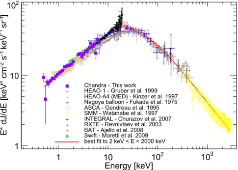
(5) The Astrophysical Journal, 837:19 (8pp), 2017 March 1. Cappelluti et al.. Figure 3. Magenta squares are the full CXB measured in this work using Chandra data from the COSMOS field (with local soft components subtracted), compared with previous results over the 0.3–1000 keV energy range and the best fit of Ajello et al. (2008). Green circles are from Moretti et al. (2009), gray crosses are the HEAO–1 measurements of Gruber et al. (1999) and Kinzer et al. (1997), red crosses are the Swift–BAT measurements from Ajello et al. (2008), black crosses are RXTE measurements from Revnivtsev et al. (2003), blue crosses are INTEGRAL measurements from Churazov et al. (2007), yellow crosses are SMM measurements from Watanabe et al. (1998), pale green open circles are ASCA measurements from Gendreau et al. (1995), and blackcrosses >100 keV are from the Nagoya balloon experiment of Fukada et al. (1975).. tails and contaminates our results. We have therefore extracted the spectrum of all the galaxies inside the mask, fit it with a simple absorbed power-law model (properly taking into account the different thermal background components in the fit), and found a spectral slope G ~ 1.3 0.06 and normalization K=3.38±0.14. We rescaled the normalization to take into account the fraction of flux falling out of the mask. Such a renormalization has been computed in the following way: we estimated, given a circular area of 3 2, the area-. Table 2 CXB Fluxes BAND keV 0.5–1.0 1.0–2.0 0.5–2.0 2.0–10.0. Total erg s−1 cm−2 deg−2. Local erg s−1 cm−2 deg−2. +0.16 5.380.15 +0.03 4.550.03 +0.16 9.950.18 +0.05 20.340.06. +0.18 2.560.18 +0.01 0.050.01 +0.23 2.290.21 0. Extragal. +0.07 3.130.07 +0.05 4.520.05 +0.11 7.620.11 +0.05 20.340.06. 3.2¢. Note. In units of 10−12 erg s−1 cm−2 deg−2.. weighted mean off-axis angle áqñ =. Extragal. erg s−1 cm−2 deg−2. %CXB. 1.24 0.17 1.66 0.06 2.90 0.16 6.47 0.82. 23.0±3.2 36.5±0.1 30.1±1.7 31.8±4.0. uCXB 0.5-1.0 1.0-2.0 0.5-2.0 2.0-10.0 nsCXB 0.5-1.0 1.0-2.0 0.5-2.0 2.0-10.0. +0.13 0.360.11 +0.07 0.610.07 +0.18 0.970.16 +1.42 3.45-1.19. 3.2¢. ò0 pq 2dq. =2 25. At. this off-axis angle, an average of 95% EEF is masked. Hence, we renormalized the galaxy spectrum by a factor of 0.95 and simulated a spectrum taken from the rescaled best fit, accounting for all the observational parameters. We subtracted the simulated spectrum from the nsCXB spectrum to remove the best possible estimate of PSF tails. Due to lower statistics, to fit such a spectrum we doubled the binning with respect to the cases above. This is because we have chosen a binning that allowed having at least 30 counts/bin. In Figure 1 we show the spectrum of the nsCXB. The spectrum has high S/N up to an energy of 5–6 keV, above which the signal is very noisy. We allowed all parameters to vary freely, but because of the low statistics, the soft thermal component is detected but not significantly required. The resulting best-fit parameters are Γ=1.25±0.35 and normalization KPL=1.37±0.30. This +1.6 corresponds to 9.71.8 % of the total CXB in the [0.5–2] keV band. This unresolved CXB fraction is about double above 2 keV. Our normalization of this unresolved component is in agreement with Hickox & Markevitch (2007) and Moretti et al. (2012), while our estimated slope is in agreement with Hickox & Markevitch (2007) but significantly softer than the Moretti et al. (2012) estimate. In Table 3 we show the extragalactic component flux of the nsCXB in several energy bands. With our masking, the. Table 3 Unresolved Extragalactic CXB Fluxes BAND keV. ò0 q * pq 2dq. +3.0 6.72.8 +1.6 13.41.6 +1.6 9.71.8 +5.9 17.07.0. Note. In units of 10−12 erg s−1 cm−2 deg−2.. 3.3. Non-source CXB Spectrum The extracted nsCXB cannot be directly used as is, since we know that up to 10% of the flux from galaxies is in the PSF 5.
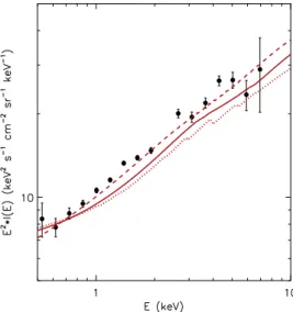
(6) The Astrophysical Journal, 837:19 (8pp), 2017 March 1. Cappelluti et al.. Figure 4. Unfolded CXB spectrum measured by Chandra with ACIS-I (black) in this work. Overplotted on the data we show AGN population synthesis models, after adding cluster emission (Gilli et al. 1999) and star-forming galaxy emission (Cappelluti et al. 2016) by Treister et al. (2009; red dotted line), Gilli et al. (2007; red continuous line), and Ballantyne et al. (2011; red dashed line). The extragalactic CXB spectrum is well fitted by a power-law model with photon index Γ∼1.45 and normalization ∼10.91 keV cm2 s−1 sr−1.. Figure 5. Spectrum of the uCXB (circles) as measured with Chandra ACIS-I in this work. The uCXB spectrum is compared with AGN synthesis models by Treister et al. (2009; red dotted line), Gilli et al. (2007; red continuous line) and Ballantyne et al. (2011; red dashed line) after the survey’s X-ray-selection function is applied (galactic NH correction is irrelevant).. Interestingly, the only model that reproduces the whole uCXB is the Gilli et al. (2007) one while that of Treister et al. (2009) is consistent with the hard X-rays. This consistency at high energy is not surprising since both models aimed to explain the peak of the CXB at high energy, and although they used different ingredients, they included a large number of hard, Compton-thick objects. The Ballantyne et al. (2011) model underpredicts the fraction of uCXB, implying that their model contains more bright sources than the other models. These discrepancies are likely due to the different assumptions for the NH distribution and luminosity functions adopted. Given the quality of the CXB data we present here and the consistent CXB levels measured by Chandra and XMM-Newton, a new population synthesis model may be warranted. According to our analysis, ∼8%–11% of the measured [0.5–2] keV CXB cannot be explained by either resolved X-ray sources or faint, unresolved sources originating in visible red galaxies that have escaped detection. Cappelluti et al. (2012, 2013) and Helgason et al. (2014) studied the fluctuations of the u/nsCXB in the deep CDFS and EGS, and concluded that these fluctuations arise from undetected groups and star-forming galaxies and a small fraction of AGNs. A detailed analysis of the fluctuations of the u/nsCXB will be presented in Li et al. (2017, in preparation). Here, we remove even fainter sources than Cappelluti et al. (2013) and Helgason et al. (2014), down to iAB ~ 27–28. Assuming that all the diffuse emission from faint groups has been removed by our galaxy masking, what is left arises from very faint undetected/ blurred point sources. In order to evaluate the contribution of star-forming galaxies to the CXB and uCXB, we used simulations of the CANDELS GOODS-South area from Cappelluti et al. (2016), which reaches optical/NIR magnitudes as faint as 30. They predict for every galaxy a value of LX concordant with the scaling relation with the SFR (approximated by the infrared luminosity) of Basu-Zych et al. (2013). Without going into details, they estimate L8–1000μm using photo-z, star-formation rate, UVJ restframe colors, and (observed or extrapolated) UV luminosity (1500 Å ). Using their mock catalog, we applied a selection as. fraction of CXB remaining varies between ∼6% at very soft energies to 17% at very high energies. 4. Discussion Ordinary populations of Type I and Type II AGNs alone cannot explain the shape and amplitude of the extragalactic CXB spectrum, especially the peak at ∼30 keV (Comastri et al. 1995; Gilli et al. 2001; Treister & Urry 2005; Gilli et al. 2007; Treister et al. 2009; Ballantyne et al. 2011). Instead, this peak is attributed to a large population of mostly undetected Comptonthick sources that are naturally missed by <10 keV X-ray surveys. In Figure 4 we compare our data with the predictions of the CXB AGN population synthesis models that have animated the scientific debate in the last 10 years (Treister & Urry 2005; Gilli et al. 2007; Treister et al. 2009; Ballantyne et al. 2011; Ueda et al. 2014). Star-forming galaxies were modeled by assuming a power law with photon index Γ=2 and a normalization of 0.55 keV cm2 s−1 sr−1 keV−1, estimated using the prescription of Cappelluti et al. (2016, see below). In that figure, we present the extragalactic CXB unfolded spectrum; although such a plot is model dependent, this is still a good approximation for the purpose of comparing with the model. A cluster model component from Gilli et al. (1999) has been added to each of these spectra. The three models reproduce the shape of the extragalactic CXB spectrum above 0.5 keV but systematically underestimate the normalization by 10%–15%. This is likely due to the intrinsic normalization chosen as a reference for these models. Differences among the models are of the order of the precision of our measurement. A valuable test of the goodness of the assumptions of population synthesis models derives from whether they are able to reproduce the uCXB at any given flux limit. In Figure 5 we compare the uCXB spectrum with the predictions of Treister et al. (2009), Gilli et al. (2007), and Ballantyne et al. (2011) at the flux limit of COSMOS (models assume an all-sky coverage, and we did not apply any correction for cosmic variance). 6.
(7) The Astrophysical Journal, 837:19 (8pp), 2017 March 1. Cappelluti et al.. similar as possible to that of Laigle et al. (2016) from which we derived our mask. As a result, we find that these galaxies produce a [0.5–2] keV CXB surface brightness of the order of 3.3×10⁻¹⁴ erg cm2 s−1 deg−2, which explains about 5% of the nsCXB. By assuming a typical X/O=0 for AGNs as determined by Civano et al. (2012) and the i-limiting magnitudes in COSMOS (Scoville et al. 2007b), we estimate that the undetected AGN [0.5–2] flux is <10−17 erg cm2 s−1. At these low fluxes, star-forming galaxies vastly outnumber AGNs, so we can assume that ordinary AGNs cannot contribute more than galaxies to the soft nsCXB (5%). Being so faint, the sources producing the remaining CXB can be local (z∼1–3) and of low luminosity. Low-luminosity AGNs are preferentially highly absorbed (Barger et al. 2005; Hasinger 2008), and therefore we could argue that the hard portion of the nsCXB could be explained by these sources. However, at z∼36, the number density of absorbed sources is still unknown, and we cannot exclude an unpredicted large number of such sources at that redshift. We propose that a large fraction of the remaining emission could arise from still undetected, rapidly accreting black holes at z>6–7. Assuming the Direct Collapse black hole (DCBH) scenario for the formation of early black hole seeds, Pacucci et al. (2015) showed that these sources are likely undetected in current deep X-ray/NIR surveys. They compared the emission of DCBHs for two accretion models: radiatively efficient (Standard) and radiatively inefficient (Slim Disk; super-Eddington), in which photon trapping is significant and the outgoing radiation is diminished. In the latter case, the luminosity emitted by these sources is low. These short-lived and fainter black holes are more difficult to detect compared to brighter objects accreting at the Eddington limit (two tentative detections were proposed by Pacucci et al. 2016). Indeed, Comastri et al. (2015) revised the estimate of the local accreted mass density by taking into account that a significant fraction of the local black holes may have grown by radiatively inefficient accretion. From our measurements, the maximum flux produced by accretion onto early black holes is ∼10% of the CXB (see Table 3). To place limits on the amount of accretion occurring at z 6, we follow the formalism of Salvaterra et al. (2012), assuming that the comoving specific emissivity of AGNs can be factorized as j (E , z) = j f (z) g (E ) ,. Table 4 Limits to the Density of Accretion at z 6 from the Unresolved Background Accretion Disk. 4pJE0 H0 W1m 2 ⎡ ⎢⎣ c. òz¯. ¥. dz (1 + z)-5. 2 - g g (E. 10−3 10−2 10−3 10−2. 6.1 ´ 10 3 1.7 ´ 10 6 6.8 ´ 10 3 6.5 ´ 10 4. where JE0 is the emissivity observed at energy E0 today, and j (E, z) on the other hand is the emissivity of all AGNs at redshift z. Note that E is in the rest frame, and E0 is the energy observed at z=0. Wm is the matter density parameter and H0 is the Hubble constant. The standard Soltan argument states that the mass density of accretion onto sources at redshifts z z¯ is given by racc (z¯) =. 1- c 2. òz¯. ¥. dz. dt dz. ò0. ¥. dEj (E , z) ,. (3 ). where ò is the radiative efficiency (0.1 and 0.04 for a standard and a slim disk, respectively. Finally, our limit on accretion at z z¯ is given by racc (z¯) =. ⎤ 4pJE0 1 - ⎡ ¥ dz (1 + z)-5 2 - g ⎥ ⎢⎣ 3 ⎦ z¯ c ¥ ⎤-1 ⎡ dz (1 + z)-5 2 - g g (E 0 (1 + z)) ⎥ . ´⎢ ⎦ ⎣ z¯. ò. ò. (4 ). Assuming that the unresolved 1.5 keV flux is entirely due to DCBHs at z 6, the inferred accretion density (r•) using these spectra is provided in Table 4. These limits are compared to those found in previous studies in Figure 6. Red, orange, green, and purple upper limits correspond to standard low-metallicity, slim disk low-metallicity, standard high-metallicity, and slim disk high-metallicity templates, respectively. In gray, we display limits from previous studies. The straight, dashed, dotted, and dotted–dashed error bars correspond to measurements from Hopkins et al. (2007), Salvaterra et al. (2012), Treister et al. (2009), and Treister et al. (2013), respectively. The gray square corresponds to local measurements by Shankar et al. (2009). Our results emphasize that limits to black hole accretion are dependent entirely on the bolometric correction assumed, and this can vary significantly from model to model. Again, while previous studies have assumed a constant fraction of total flux emitted in the observed window, we calculated this fraction directly from hydrodynamical simulations. These models imply that much less accretion is required to provide the observed flux if gas is accreted from a lower-metallicity reservoir Z = 10-3, while larger metallicities Z > 10-2 would exceed the z∼5–6 accreted density of Hopkins et al. (2007). The limits in the lower-metallicity case are comparable to or more stringent than what is obtained with stacking analysis in Treister et al. (2013; r• 10 3 M Mpc-3). Cappelluti et al. (2013) determined that the unresolved nsCXB and unresolved cosmic infrared background fluctuations are highly correlated (see, e.g., Kashlinsky et al. 2012). Yue et al. (2013) interpreted this as a signature of emission from a population of DCBHs at z>12. In order to satisfy the observed cross-power and not to exceed the nsCXB measured. (1 ). 0 (1. r• (M Mpc-3). Standard Standard Slim Disk Slim Disk. where j is the normalization, f (z ) = (1 + z )-g , with g » 5, is the redshift evolution, and g(E) is a (normalized) template spectrum. For these templates, we use AGN spectra generated by realistic hydrodynamical simulations of accreting DCBHs (Pacucci et al. 2015). These templates allow us, essentially, to compute the bolometric correction needed for the Soltan argument as a function of redshift. For each value of the gas metallicity and accretion model (Standard or Slim Disk), we select the spectrum from the snapshot with the highest X-ray output. Combining Equation (1) with knowledge of the contribution to the background at energy E0 by sources at redshifts z z¯ , the normalization can be solved: j =. Metallicity (Z ). ⎤-1 + z)) ⎥ , ⎦ (2 ). 7.
(8) The Astrophysical Journal, 837:19 (8pp), 2017 March 1. Cappelluti et al. Bartalucci, I., Mazzotta, P., Bourdin, H., & Vikhlinin, A. 2014, A&A, 566, A25 Basu-Zych, A. R., Lehmer, B. D., Hornschemeier, A. E., et al. 2013, ApJ, 762, 45 Capak, P., Aussel, H., Ajiki, M., et al. 2007, ApJS, 172, 99 Cappelluti, N., Brusa, M., Hasinger, G., et al. 2009, A&A, 497, 635 Cappelluti, N., Comastri, A., Fontana, A., et al. 2016, ApJ, 823, 95 Cappelluti, N., Kashlinsky, A., Arendt, R. G., et al. 2013, ApJ, 769, 68 Cappelluti, N., Ranalli, P., Roncarelli, M., et al. 2012, MNRAS, 427, 651 Churazov, E., Sunyaev, R., Revnivtsev, M., et al. 2007, A&A, 467, 529 Civano, F., Elvis, M., Brusa, M., et al. 2012, ApJS, 201, 30 Civano, F., Marchesi, S., Comastri, A., et al. 2016, ApJ, 819, 62 Comastri, A., Gilli, R., Marconi, A., Risaliti, G., & Salvati, M. 2015, A&A, 574, L10 Comastri, A., Setti, G., Zamorani, G., & Hasinger, G. 1995, A&A, 296, 1 De Luca, A., & Molendi, S. 2004, A&A, 419, 837 Dickey, J. M., & Lockman, F. J. 1990, ARA&A, 28, 215 Elvis, M., Civano, F., Vignali, C., et al. 2009, ApJS, 184, 158 Fukada, Y., Hayakawa, S., Kasahara, I., et al. 1975, Natur, 254, 398 Gendreau, K. C., Mushotzky, R., Fabian, A. C., et al. 1995, PASJ, 47, L5 Gilli, R., Comastri, A., & Hasinger, G. 2007, A&A, 463, 79 Gilli, R., Risaliti, G., & Salvati, M. 1999, A&A, 347, 424 Gilli, R., Salvati, M., & Hasinger, G. 2001, A&A, 366, 407 Gruber, D. E., Matteson, J. L., Peterson, L. E., & Jung, G. V. 1999, ApJ, 520, 124 Hasinger, G. 2008, A&A, 490, 905 Helgason, K., Cappelluti, N., Hasinger, G., Kashlinsky, A., & Ricotti, M. 2014, ApJ, 785, 38 Hickox, R. C., & Markevitch, M. 2006, ApJ, 645, 95 Hickox, R. C., & Markevitch, M. 2007, ApJL, 661, L117 Hopkins, P. F., Richards, G. T., & Hernquist, L. 2007, ApJ, 654, 731 Humphrey, P. J., Liu, W., & Buote, D. A. 2009, ApJ, 693, 822 Ilbert, O., Capak, P., Salvato, M., et al. 2009, ApJ, 690, 1236 Kashlinsky, A. 2016, ApJL, 823, L25 Kashlinsky, A., Arendt, R. G., Ashby, M. L. N., et al. 2012, ApJ, 753, 63 Kinzer, R. L., Jung, G. V., Gruber, D. E., et al. 1997, ApJ, 475, 361 Laigle, C., McCracken, H. J., Ilbert, O., et al. 2016, arXiv:1604.02350 Leccardi, A., & Molendi, S. 2007, A&A, 472, 21 Marchesi, S., Civano, F., Elvis, M., et al. 2016, ApJ, 817, 34 Markevitch, M., Bautz, M. W., Biller, B., et al. 2003, ApJ, 583, 70 McCammon, D., Almy, R., Apodaca, E., et al. 2002, ApJ, 576, 188 Miyaji, T., Ishisaki, Y., Ogasaka, Y., et al. 1998, A&A, 334, L13 Moretti, A., Campana, S., Lazzati, D., & Tagliaferri, G. 2003, ApJ, 588, 696 Moretti, A., Pagani, C., Cusumano, G., et al. 2009, A&A, 493, 501 Moretti, A., Vattakunnel, S., Tozzi, P., et al. 2012, A&A, 548, A87 Pacucci, F., Ferrara, A., Grazian, A., et al. 2016, MNRAS, 459, 1432 Pacucci, F., Ferrara, A., Volonteri, M., & Dubus, G. 2015, MNRAS, 454, 3771 Puccetti, S., Vignali, C., Cappelluti, N., et al. 2009, ApJS, 185, 586 Revnivtsev, M., Gilfanov, M., Sunyaev, R., Jahoda, K., & Markwardt, C. 2003, A&A, 411, 329 Salvaterra, R., Haardt, F., Volonteri, M., & Moretti, A. 2012, A&A, 545, L6 Scoville, N., Abraham, R. G., Aussel, H., et al. 2007a, ApJS, 172, 38 Scoville, N., Aussel, H., Brusa, M., et al. 2007b, ApJS, 172, 1 Shankar, F., Weinberg, D. H., & Miralda-Escué, J. 2009, ApJ, 640, 20 Treister, E., Schawinski, K., Volonteri, M., & Natarajan, P. 2013, ApJ, 778, 130 Treister, E., & Urry, C. M. 2005, ApJ, 630, 115 Treister, E., Urry, C. M., & Virani, S. 2009, ApJ, 696, 110 Ueda, Y., Akiyama, M., Hasinger, G., Miyaji, T., & Watson, M. G. 2014, ApJ, 786, 104 Verner, D. A., Ferland, G. J., Korista, K. T., & Yakovlev, D. G. 1996, ApJ, 465, 487 Watanabe, K., Leising, M. D., Hartmann, D. H., & The, L.-S. 1998, AN, 319, 67 Wilms, J., Allen, A., & McCray, R. 2000, ApJ, 542, 914 Worsley, M. A., Fabian, A. C., Barcons, X., et al. 2004, MNRAS, 352, L28 Yue, B., Ferrara, A., Salvaterra, R., Xu, Y., & Chen, X. 2013, MNRAS, 433, 1556. Figure 6. Comparison of our limits to previous studies. Red, orange, green, and purple bars represent our standard low-metallicity, slim disk low-metallicity, standard high-metallicity, and slim disk high-metallicity limits, respectively. In gray, the solid, dashed, dotted, and dotted–dashed error bars correspond to previous measurements by Hopkins et al. (2007), Salvaterra et al. (2012), Treister et al. (2009), and Treister et al. (2013). The gray square around redshift 0 corresponds to the local estimate by Shankar et al. (2009). Our study emphasizes that the assumed model dramatically changes the bolometric correction used, and therefore the limits on the accreted mass density.. here, their envelopes must be Compton-thick. With our new limits on the nsCXB, according to Yue et al. (2013) DCBHs must have NH >1.6×1025 cm−2. To summarize, if this population of early massive black holes exists, the black holes had to grow in Compton-thick, low-metallicity environments. N.C. acknowledges Yale University’s YCAA Prize Postdoctoral fellowship. N.C., G.H., Y.L., and F.P. acknowledge the SAO Chandra grant AR6-17017B and NASA-ADAP grant MA160009. P.N. acknowledges support from a Theoretical and Computational Astrophysics Network grant with award number 1332858 from the National Science Foundation. B.A. and A.R. acknowledge support from the TCAN grant for a postdoctoral fellowship and a graduate fellowship, respectively. A.C. and R.G. acknowledge PRIN INAF 2014 Windy black holes combing galaxy evolution and ASI/INAF grant I/037/12/0 011/13. E.T. acknowledge support from FONDECYT regular grant 1160999 and Basal-CATA PFB-06. This work is part of the NASA Project “LIBRAE: Looking at Infrared Background Radiation Anisotropies with Euclid” (http://librae.ssaihq.com). We thank the anonymous referee for the useful insights and suggestions. References Ajello, M., Greiner, J., Sato, G., et al. 2008, ApJ, 689, 666 Arnaud, K. A. 1996, adass V, 101, 17 Ballantyne, D. R., Draper, A. R., Madsen, K. K., Rigby, J. R., & Treister, E. 2011, ApJ, 736, 56 Barger, A. J., Cowie, L. L., Mushotzky, R. F., et al. 2005, AJ, 129, 578. 8.
(9)
Figure

Documento similar