PHASE RESOLVED NuSTAR AND SWIFT XRT OBSERVATIONS OF MAGNETAR 4U 0142+61
13
0
0
Texto completo
(2) The Astrophysical Journal, 808:32 (13pp), 2015 July 20. Tendulkar et al. Table 1 X-Ray Observations of 4U 0142+61 in 2014. unexceptional source until 8.7 s X-ray pulsations were discovered by ASCA (Israel et al. 1993, 1994). The soft X-ray emission from 4U 0142+61 is well described by a blackbody with k B T ~ 0.4 keV and a power law (PL) with index G ~ 3.7 (White et al. 1996; Israel et al. 1999; Paul et al. 2000; Juett et al. 2002; Patel et al. 2003; Göhler et al. 2004, 2005; Rea et al. 2007; Enoto et al. 2011). Pulsed highenergy emission was detected between 20–50 and 50–100 keV using the IBIS/ISGRI instrument on INTEGRAL (den Hartog et al. 2004). The hard X-ray spectrum (>10 keV) is dominated by a PL component with G ~ 1 (den Hartog et al. 2006; Kuiper et al. 2006; den Hartog et al. 2008b; Enoto et al. 2011). Using upper limits on the γ-ray flux from the CGRO-COMPTEL telescopes, the hard X-ray PL cutoff energy was suggested to be between ∼200–750 keV (Kuiper et al. 2006). The soft X-ray pulse profiles of 4U 0142+61 were shown to undergo long-term changes using RXTE observations spread over 10 years (Dib et al. 2007) and later Chandra, XMMNewton and Swift observations (Gonzalez et al. 2010). The pulse fractions were observed to increase over time leading up to a group of three bursts that occured between 2006 and 2007 (Gonzalez et al. 2010). There has been much debate about the intrinsic soft X-ray spectra of magnetars, the measurement of which depends on the absorption column, NH, along the line of sight. Durant & van Kerkwijk (2006b), hereafter D06b, estimated the NH to 4U 0142+61 to be (6.4 0.7) ´ 10 21 cm-2 by fitting highresolution grating spectra around individual photoelectric absorption edges of oxygen, iron, neon, magnesium and silicon. They also showed that the abundance ratios of Ne/ Mg and O/Mg for 4U 0142+61 are closer to the revised solar abundances of Asplund et al. (2005) compared to the old standard abundances of Anders & Grevesse (1989). This measurement has the advantage of being less sensitive to the choice of model used to describe the intrinsic magnetar spectrum. However, since only the data near photo-electric edges is fitted, the fitting requires high-quality X-ray data. Unlike the NH measurements from the high-resolution X-ray spectra, most fits of the low-energy spectrum (≈0.5–10 keV) with a blackbody plus PL model converge to NH » 1.0 ´ 1022 cm-2 (Rea et al. 2007, and references therein) which used the abundances from Anders & Grevesse (1989). We note that Enoto et al. (2011) obtained NH values consistent with the D06b value from broadband spectral fits to Suzaku data, however, no abundance model was specified. In this work, we use solar abundance values from Asplund et al. (2009)—the “aspl” model in XSPEC—as default, and we also test our fits with other abundance models. By identifying core helium-burning giant stars—i.e., red clump stars—from the 2MASS catalog and estimating the variation of optical extinction as a function of distance in the direction of magnetars, Durant & van Kerkwijk (2006a) estimated the distance to 4U 0142+61 to be 3.6 ± 0.4 kpc. This distance estimate used the NH = (6.4 0.7) ´ 10 21 cm-2 estimated from the photo-electric absorption edges. Previous measurements of optical extinction (AV) have concluded that the AV for 4U 0142+61 should be less than 5 (Hulleman et al. 2004; Durant & van Kerkwijk 2006b), corresponding to NH < 9 ´ 10 21 cm-2 (Predehl & Schmitt 1995, AV = NH ´ 5.6 ´ 10 22 cm2 ). In this paper, we present a phase-resolved spectral and timing analysis of coordinated Swift-X-ray Telescope (XRT). Obs ID. Start (UT). NuSTAR 30001023002 Mar 27 13:35 30001023003 Mar 28 00:45 Swift-XRT (Windowed Timing Mode) 00080026001 Mar 27 13:36 00080026002 Mar 28 07:10 00080026003 Mar 30 00:42. End (UT). Exp (ks). Ratea cts/s. Mar 28 00:45 Mar 30 13:00. 7 37. 1.3 1.3. Mar 27 21:52 Mar 29 23:15 Mar 30 08:57. 4.9 12.9 6.6. 4.2 4.0 4.1. Note. a 0.5–10 keV count rate for Swift-XRT and 3–79 keV count rate from NuSTAR.. and NuSTAR spectra of 4U 0142+61. We use the Hascoët et al. (2014) framework to test the electron–positron outflow model and constrain physical parameters. The paper is organized as follows. In Section 2, we describe our observations, data and data reduction procedure. In Section 3, we describe the results of our timing analysis, spectral analysis and model fitting. In Section 4, we discuss these results in the context of previous observations of 4U 0142+61 and those of other magnetars. 2. OBSERVATIONS AND ANALYSIS NuSTAR (Harrison et al. 2013) is a 3–79 keV focusing hard X-ray mission. It consists of two identical co-aligned Wolter-I telescopes with CdZnTe detectors at the focal planes. The telescopes provide a point-spread function with a half-power diameter of 58″ over a field of view of 12′ × 12′. The energy resolution varies from 0.4 keV at 6 keV to 0.9 keV at 60 keV. The two focal plane modules are referred to as FPMA and FPMB. 4U 0142+61 was observed by NuSTAR between 2014 March 27 and 30 during a 44 ks observation simultaneous with a 24 ks observation with the Swift XRT (Burrows et al. 2005). The details of the observations are summarized in Table 1. We performed the processing and filtering of the NuSTAR event data with the standard NuSTAR pipeline version 1.4.1 and HEASOFT version 6.16. We used the barycorr tool to correct the photon arrival times for the orbital motion of the satellite and the Earth at the optical position of 4U 0142 +61—a = 01h 46m22.s 407, d = +6145¢03. 19 (J2000)—as reported by Hulleman et al. (2004). The source events were extracted within a 50 pixel (120″) radius around the centroid and suitable background regions were used. Spectra were extracted using the nuproducts script. Using grppha, all photons below channel 35 (3 keV) and above channel 1935 (79 keV) were flagged as bad and all good photons were binned in energy to achieve a minimum of 30 photons per bin. The Swift-XRT data were obtained in the Windowed Timing (WT) mode and were processed with the standard xrtpipeline and the photon arrival times were corrected using barycorr. The xrtproducts script was used to extract spectra and lightcurves within a radius of 25 pixel (59″).14 Photons in channels 0–29 (energy <0.3 keV) were ignored and all channels between 0.3 and 10 keV were binned to ensure a minimum of 30 photons per bin. The Swift-XRT and NuSTAR FPMA and FPMB spectra were fit simultaneously in XSPEC v12.8.1 (Arnaud et al. 1996) 14. As per the Swift-XRT data analysis thread: http://www.swift.ac.uk/analysis/ xrt/spectra.php.. 2.
(3) The Astrophysical Journal, 808:32 (13pp), 2015 July 20. Tendulkar et al.. Figure 1. Swift-XRT and NuSTAR pulse profiles in different energy bands. The annotation in the upper left corner of each plot specifies the telescope (“S”: Swift-XRT, “N”: NuSTAR) and the energy band for each plot. The last plot is the total 0.3–79 keV (Swift-XRT and NuSTAR) count rate (normalized to the average value) marked with phase bins—“A,” “B” and “C” and “DC”—used for fitting the e--e+ outflow model (Section 3.7). Two pulse periods are shown for clarity.. using two freely varying cross-normalization constants, assuming the normalization of Swift-XRT to be fixed to unity. Timing analysis was performed on exposure-corrected lightcurves and event lists using custom MATLAB scripts.. approximately equal counts in each band. The 3–5 and 5–8 keV data from Swift-XRT had far lower count rates than the corresponding NuSTAR observations and hence were not used for the final analysis. However, we confirmed that the NuSTAR and Swift-XRT pulse profiles in these two overlapping energy bands are consistent within the error bars. There is a clear gradual change in the pulse morphology as the energy band crosses ∼3 and ∼20 keV, corresponding to the different spectral components—modified blackbody or hard PL —that dominate the spectrum at these energies. This change in morphology is also observed in the dominance of the Fourier harmonics described in Section 3.2. The 0.3–1.5 and 1.5–3 keV pulse profiles consist of two peaks at phases of ϕ = 0.3 and ϕ = 0.6 separated by a sharp dip at ϕ = 0.5. In the 3–5 and 5–8 keV bands, the peak at ϕ = 0.3 dominates the pulse and the dip at ϕ = 0.5 deepens significantly. There is a small dip at ϕ = 0.9 separating a possible second pulse peak from the primary. Moving to higher photon energies, in the 8–20 and 20–35 keV bands, a second pulse rises in amplitude at f » 0.65 toward energies of 50 keV. The primary pulse also shows signs of broadening as a function of energy.. 3. RESULTS 3.1. Pulse Profile We analyzed the barycentered 3–79 keV NuSTAR events using epoch folding (Leahy 1987) and measured the rotation period of 4U 0142+61 to be P = 8.689158(4) s. This is consistent with the period measured with the Swift-XRT observation and is also consistent with the period P = 8.689163(5) s expected at the epoch of observation based on the last ephemeris measured after the glitch of 2011 July, reported by Dib & Kaspi (2014). We folded the Swift-XRT and NuSTAR events in eight energy bands into 20 phase bins with our measured period to compare the pulse morphology as a function of energy (Figure 1). The energy bands—0.3–1.5, 1.5–3, 3–5, 5–8, 8–20, 20–35, 35–50 and 50–79 keV—were chosen to have 3.
(4) The Astrophysical Journal, 808:32 (13pp), 2015 July 20. Tendulkar et al.. whereas the fraction of power in the second harmonic ( A2 Atotal ) increases with energy until approximately 40 keV and then decreases. This behavior of the harmonics is significantly different from that of 1E 2259+586 presented in Vogel et al. (2014). In 1E 2259+586, the normalized A1 value increases as a function of energy until approximately 12 keV and then decreases as a function of energy. The normalized value of A2 decreases as a function of energy until approximately 12–15 keV and then increases. 3.3. Pulse Fraction We quantify the strength of the pulsations using two different methods. We define the rms pulse fraction as 2 å k =1 N. PFrms = Figure 2. Variation in the first (filled symbols) and second (empty symbols) harmonic amplitudes as a function of photon energy. Both values are normalized with respect to the total amplitude of the variation (Atotal). The Swift-XRT data points are shown as red circles and the NuSTAR data points are shown as black squares. The filled areas (solid for A1 Atotal and hashed for A2 Atotal ) show the 1-σ error regions.. bk =. N. j=1. 1 N. æ 2pkj ö ÷÷ and N ÷ø. (1). æ 2pkj ö ÷÷ N ÷ø. (2). N. å p j sin çççè j=1. )). ,. (4). 1 N2. å sp2. sb2k =. 1 N2. å sp2. j=1. j. N. j=1. j. æ 2pkj ö ÷, cos2 çç çè N ÷÷ø. (5). æ 2pkj ö ÷. sin2 çç çè N ÷÷ø. (6). å j =1 p j. ( ).. - N * min p j. å j =1 p j N. (7). This definition is consistent with that used by dH08. However, it is challenging to determine the true value of min(p j ), and both noise and binning tend to bias the PFarea metric upwards by as much as 20% (An et al. 2015). Figure 3 shows the variation of PFarea (filled symbols) and PFrms (empty symbols) as a function of energy. Note that while our measurements of PFarea have an increasing trend at energies >10 keV, the PFarea values above 20 keV are also consistent with a constant value of ≈35%. The near-linear increase in PFarea as a function of energy is consistent with the results of dH08, though we note that our PFarea measurements are consistently higher than those of dH08 and those of Gonzalez et al. (2010). The rms pulse fraction, PFrms, increases with energy up to an energy of 35 keV. However, the absolute normalization is different due to the different definitions of pulse fractions. The possible decrease in PFrms in the 35–50 and 50–79 keV bands may be due to the emergence of two nearly equal amplitude peaks in the pulse profile with lower count rates. A similar reduction in rms pulsed fraction with energy had been reported for 1E 1841–045 in the 16–24 keV band observations (An et al. 2013). However, with more NuSTAR observations the variations were shown to be dependent on the exact energy bins used (An et al. 2015).. N. å A k2 .. N. sa2k =. N. where N is the number of phase bins and pj is the number of photons in each phase binand j and k are indices referring to the phase bins and the Fourier harmonics respectively. We define the strength of each Fourier component to be Ak = a k2 + b k2 . We define Atotal as A total =. a0. PFarea =. To explore the variation in pulse shape as a function of energy, we decomposed the pulses into Fourier harmonics. We define Fourier coefficients ak and bk as. å p j cos çççè. ) (. + b k2 - sa2k + sb2k. This definition, including the correction term, sa2k + sb2k , has been shown to be a robust and accurate metric of pulse fraction in noisy data (see Appendix 1 of An et al. 2015, for a detailed discussion). We also define the area pulse fraction described by Gonzalez et al. (2010) as. 3.2. Pulse Morphology. 1 N. 2 k. where ak and bk are as defined above and sa k and sb k are the uncertainties in ak and bk, respectively, calculated using Poisson variances as. Our low-energy results are consistent with the RXTE observations reported by den Hartog et al. (2008b) (hereafter dH08) and with the 0.5–10 keV XMMNewton observations of Gonzalez et al. (2010) from 2008 March. However, the 20–35 and 35–50 keV observations from NuSTAR show a double peak structure with the primary peak having approximately twice the peak amplitude as compared to the secondary peak. The corresponding INTEGRAL pulse profile reported in dH08 showed a double peak structure with both peaks of equal amplitude. This difference is also present in the pulse fraction analysis presented in Section 3.3.. ak =. ( (a. (3). k= 1. We find that most of the variational power in the pulses is explained in the first six harmonic coefficients. The distinct variation of pulse shapes with energy can be seen in Figure 2. The fraction of power in the first harmonic ( A1 Atotal ) decreases with energy until approximately 40 keV and then increases, 4.
(5) The Astrophysical Journal, 808:32 (13pp), 2015 July 20. Tendulkar et al.. Figure 4. Variation of Z 42 as a function of rotation period for 4U 0142+61 for 15–40 keV band using NuSTAR data (solid black curve) overlaid on SuzakuHXD results from ME14 (red dashed and solid curves). We find that Z 42 peaks to a value of »360 at the measured rotation period of 8.689158 s (Section 3.1). The dotted red line is Z 42 for the raw (non-demodulated) Suzaku-HXD data reported in Figure 1b of ME14. The solid red line is Z 42 for the same HXD data after optimal demodulation. The vertical dashed red line is the high-energy (15–40 keV) rotational period reported by ME14 with the shaded region denoting the reported error and the vertical dashed red line the low-energy (0.3–10 keV) rotational period reported from the XIS data for the same epoch. Vertical black lines are the expected rotation periods for the 2009 August and 2014 March epochs from the RXTE data. The rotation periods marks are offset vertically for clarity.. Figure 3. Variation in the area pulsed fraction (filled symbols) and rms pulsed fraction (empty symbols) as a function of energy. The Swift-XRT and NuSTAR symbols are the same as in Figure 2. The filled areas (solid for PFarea and hashed for PFrms) show the 1σ error regions.. The overall trend of both rms and area pulse fraction was shown to increase with energy, with PFrms increasing up to 20% at 50 keV and PFarea increasing to 50% at 50 keV. Similar to 1E 1841–045, PFrms does not show signs of increasing to 100% with increasing energy as was suggested from the INTEGRAL data (dH08).. demodulation) and Z 42 » 52 (after optimal demodulation) reported in their Figures 1(b) and (c). We searched for phase modulation in the data by shifting the arrival times of each photon by Dt = A sin(2pt T - f0 ), where t is the time of arrival, A is the modulation amplitude (with units of time), T is the modulation period and f0 is the initial phase. We measured Z 42 after varying T between 45 and 65 ks in steps of 2.5 ks, A between 0 and 1.2 s in steps of 0.1 s and f0 between 0° and 360° in steps of 20°. These results were compared to Figure 2 of ME14. We find that unlike ME14, Z 42 peaks to a value >350 at A = 0 reducing to »100 at A = 1.2. Z 42 is also nearly independent of f0 at any given T and A. We find no preference for the values of A = 0.7 0.3 s and f0 = 75 30. Assuming a 55 ks period reported by ME14, we split the data into six subsets, each 9.17 ks long, and created individual pulse profiles by folding each subset at P = 8.689158(4) s. We find no phase change between any two pulse profiles (compared to Figure 3 of ME14). We also find that the post-demodulation pulse profile reported in Figure 1(f) of ME14 is triple-peaked with PFarea 10% and significantly different from the doublepeaked NuSTAR profile and the 20–50 keV pulse profile reported from XMM-Newton data in dH08 (Figure 7(E)), each with PFarea » 30 %.. 3.4. Non-detection of Precession Makishima et al. (2014) (hereafter ME14) reported a phase modulation in the 8.7 s rotation period of 4U 0142+61 with an amplitude of 0.7 s and a period of 55±4 ks (≈15 hr) detected from 15 to 40 keV HXD-PIN data gathered with Suzaku in 2009 August. This was interpreted as possible evidence for the precession of the neutron star caused by slight deviation from spherical symmetry. The same search in Suzaku-HXD data gathered in 2007 August and XIS data from 2007 August to 2009 August did not lead to detection of precession. Since our observations are spread over 4 days, we searched for possible variations in the rotation period or rotation phase following the same Z2n analysis (Brazier 1994) steps reported by ME14. For n = 3 and n = 4, we find that Z2n peaks to a value of »360 at the rotation period of P = 8.689158(4) s for the NuSTAR data without the need for demodulation (Figure 4). This is consistent with the P = 8.689163(5) s expected from the RXTE ephemeris of 4U 0142+61 (Dib & Kaspi 2014, Ephemeris E, Table 6). From the 2009 August 12 to 14, Suzaku-XIS data, ME14 reported a period of P = 8.68891 ±0.00010 s, which is inconsistent with the value of P = 8.68869734(8) s reported from the RXTE ephemeris (Dib & Kaspi 2014, Ephemeris D, Table 6). The Suzaku-XIS and HXD measured rotation periods are marked in Figure 4 with their corresponding errors along with the RXTE ephemeris for comparison. Figure 4 indicates that in the NuSTAR observations, the pulsations were detected at a higher significance than during the high-energy Suzaku observations. This result is (a) similar in value and shape to the result reported in Figure 1(a) of ME14 (XIS data from the same Suzaku observations), (b) significantly higher than the Z 32 = 12 and Z 42 = 16 (without. 3.5. Spectral Fits The phase-averaged X-ray spectrum of 4U 0142+61 has been previously fit with a hard PL at high energies (20 keV) and by a modified blackblody (BB) or combination of blackbodies at low energies (10 keV). We fit the extracted spectrum in XSPEC with three different models: (I) a hard 5.
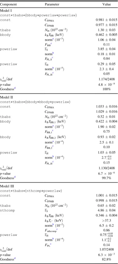
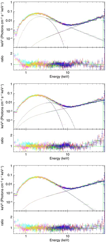
(6) The Astrophysical Journal, 808:32 (13pp), 2015 July 20. Tendulkar et al.. Table 2 Phase-averaged Spectral Fits Component. Parameter. Model I const∗tbabs∗(bbody+powerlaw+powerlaw) const CFPMA CFPMB tbabs NH (10 22 cm-2 ) bbody k B TBB (keV) norma (10−3) FBBc powerlaw GS normb FPL,Sc powerlaw GH normb (10−5) FPL,H c 2 cred dof. Model II const∗tbabs∗(bbody+bbody+powerlaw) const CFPMA CFPMB tbabs NH (10 22 cm-2 ) bbody k B TBB,1 (keV). powerlaw. Value. 0.981 ± 0.015 0.977 ± 0.015 1.30 ± 0.03 0.462 ± 0.005 1.06 ± 0.04 0.11 3.85 ± 0.04 0.18 ± 0.01 0.84 0.29 ± 0.05 2.3 ± 0.4 0.05 1.174/2408. 4.8 ´ 10-9 100%. p-value Goodnessd. bbody. 1.033 1.029 0.52 0.422. ± ± ± ±. 0.016 0.016 0.01 0.004. norma (10−3) FBB,1c k B TBB,2 (keV). 1.90 ± 0.02 0.75. norma (10−4) FBB,2 c. 2.5 ± 0.1 0.10. GH normb (10−4) FPL,H c. 1.03 ± 0.05 + 0.4 2.70.3 0.15. 0.93 ± 0.02. 2 cred dof. 1.130/2408. p-value Goodnessd. 6.7 ´ 10-6 99.7%. Model III const∗tbabs∗(nthcomp+powerlaw) const CFPMA CFPMB tbabs NH (10 22 cm-2 ) nthcomp GS k B TBB (keV) k B Te- (keV) normb (10−2) Fnthcompc powerlaw GH normb (10−4) FPLc 2 cred dof p-value Goodnessd. high-energy PL plus a blackbody and a soft low-energy PL, (II) a hard high-energy PL plus two BB models at low energies, and (III) a hard high-energy PL plus a comptonized BB (nthcomp Życki et al. 1999) at low energies. Each model included a tbabs model (Wilms et al. 2000) with solar elemental abundances (“aspl”) and cross-sections described by the “bcmc” model (Balucinska-Church & McCammon 1992; Yan et al. 1998) to fit for photo-electric absorption and a cross-normalization parameter to allow for slight calibration differences between the Swift-XRT, NuSTAR FPMA and NuSTAR FPMB detectors. In Section 3.7, we present fits to the phase-averaged spectra with a customized combination of models I and II: a sum of one blackbody, one modified blackbody with a soft PL tail and a hard PL, similar to the resonant compton scattering model used by Rea et al. (2007). The results of the fitting are shown in Table 2. We checked the validity of each model fit by generating 1000 sets of synthetic data based on the best-fit model parameters and testing their c 2 with respect to the model. If the distribution of c 2 values from synthetic data is significantly lower than the c 2 of the real data, the fit is deemed to be unacceptable. The “goodness” parameter in Table 2 shows the fraction of synthetic c 2 values that are lower than the c 2 from the real data. Models I and II have traditionally been used to describe the spectrum of 4U 0142+61. However, we find that while the models can match the spectral distribution visually, the fits are statistically unacceptable. Model III provides a statistically acceptable fit. Figure 5 shows the fit of model I (BB+2PL, top panel), model II (2BB+PL, middle panel) and model III (nthcomp +PL, bottom panel). As noted in Table 2, the index of the highenergy PL (GH ) varies between 0.3 and 1.0 depending on the model used to fit the low energy spectrum. This is reflected in the residuals at the high-energy end of Figure 5. It is clear that the best-fit high-energy PL underpredicts the data at high energy for model II (middle panel) while it over predicts the data when the <10 keV spectrum is modeled with model I (top panel). Note that while the nthcomp model is a good phenomenological fit to the low and intermediate energy X-ray spectrum and the blackbody emission from the surface is expected to be upscattered by high-energy electrons outside the neutron star, the nthcomp model does not accurately account for the effects of the extremely strong magnetic field on the photon scattering process. If we restrict the fits to the low-energy spectrum (<10 keV), model I fits improve with c 2 dof = 1554.3 1391 and the parameter values are similar (within 2σ) to those in Table 2, suggesting that this model can fit the low-energy spectrum well but cannot describe the 10–20 keV region of the spectrum. Fitting model II to the low-energy spectrum produces c 2 dof = 2082.4 1391, which is statistically unacceptable. Assuming a nominal value for the neutron star radius RNS = 10 km and a distance of 3.6 kpc (Durant & van Kerkwijk 2006a), we can calculate the fraction of the neutron star surface area (NS) covered by the blackbody of a given flux normalization. For model I, the blackbody has a bolometric luminosity of L bol = 1.3 ´ 1035 erg s-1, covering 0.2 NS and contributing 11% of the 0.5–79 keV X-ray luminosity (most of it in the 0.5–10 keV band), while the soft PL contributes the remaining 84%. For model II, the low temperature blackbody (L bol = 2.5 ´ 1035 erg s-1) covers 0.6 NS and contributes 75% of the luminosity, while the high. 1.001 ± 0.015 0.998 ± 0.015 0.65 ± 0.02 4.86 ± 0.04 0.346 ± 0.004 >37.3 6.5 ± 0.2 0.86 + 0.05 0.750.04 + 0.2 1.10.1 0.14 1.07/2408. 6.3 ´ 10-3 82.8%. Notes. a Normalization in units of L 39 D102 , where L39 is the source luminosity in units of 1039 erg s-1 and D10 is the distance to the source in units of 10 kpc. b Normalization in units of photons keV-1 cm-2 s-1 at 1 keV. c Fraction of the total 0.5–79 keV flux contributed by the component. d Goodness of fit is the percentage of c 2 values from 1000 Monte Carlo simulations synthesized the best-fit model parameters that are less than the best-fit c 2 value. The data are indistinguishable from the synthesized data if the goodness ≈50%.. 6.
(7) The Astrophysical Journal, 808:32 (13pp), 2015 July 20. Tendulkar et al.. and comptonized PL) contribute 86% of the total X-ray flux, similar to the contributions of the two blackbodies of model II. 3.5.1. High-energy PL. The differences in the hard PL between different models are caused by the inability of these phenomenological models to accurately describe the spectrum between approximately 10 and 20 keV. In order to minimize the figure-of-merit (c 2 in this case) for the fit, XSPEC forces variations in the hard PL index and normalization. To better measure the slope of the hard PL, we restricted the energy range from 20 to 79 keV and fit the phase-averaged spectrum with a PL. We measure GH = 0.65 0.09. The two parameter fit yielded a 2 = 477.12 for 492 degrees of freedom (dof) and a p-value cred of 0.68. This is independent of NH and the model used to describe the soft X-ray (<10 keV) spectrum. When the energy range is further constrained (i.e., in the ranges 25–79 and 30–79 keV), we get consistent measures of GH but with larger uncertainties. This value is lower than the GH = 0.93 0.06 measured by dH08 and GH = 0.89 0.10 measured by Enoto et al. (2011). However, note that the values measured by dH08 varied from 0.79 ± 0.10 to 1.21 ± 0.16 over different datasets. The nthcomp model provides the least structured residuals and the value of GH is closest to the high-energy-only value. If the high-energy hard PL is frozen to the GH = 0.65 value and the corresponding normalization and the low-energy (0.5–10 keV) spectrum is described with parameters from model I, the fit worsens with c 2 = 3104.0 in 2412 dof. The fit for model II also worsens with c 2 = 3061.3 in 2412 dof. Both models show structured wavy residuals between 5 and 11 keV suggesting that the models are failing to capture all the structure in the data. Model III fit parameters do not change values within 1-σ errors when the hard PL is frozen, c 2 = 2602.8 for 2412 dof and the goodness of fit is 85%. 3.5.2. Photoelectric Absorption. We note that the NH value from Model III (Table 2) is consistent with the D06b value of (6.4 0.7) ´ 10 21 cm-2 . To check on the influence of various abundance models, we retested the model fits with the seven abundance data sets used in X-ray astronomy (Table 3, in chronological order). We find that the older abundance data sets (aneb, angr) consistently provide lower NH values compared to the newer data sets (wilm,lodd, aspl) and that the nthcomp+PL model provides the better fit irrespective of which abundance model is used. Note that these values are roughly similar to the previous values reported by Patel et al. (2003) (NH = (0.93 0.02) ´ 10 22 cm-2 , using aneb abundances and Model I) and by Rea et al. (2007) (NH = (0.926 0.005) ´ 10 22 cm-2 , using angr abundances and Model I).. Figure 5. Unfolded phase-averaged Swift-XRT and NuSTAR spectrum and the ratio of the data to the model. The model fit shown is const∗tbabs∗(bbody +powerlaw+powerlaw) (Model I, top panel), const∗tbabs∗(bbody +bbody+powerlaw) (Model II, middle panel) and const∗tbabs∗ (nthcomp+powerlaw) (Model III, bottom panel). The colors are as follows: black: NuSTAR FPMA Obs I, red: NuSTAR FPMA Obs II, blue: NuSTAR FPMB Obs I, green: NuSTAR FPMB Obs II, cyan, yellow, magenta: Swift-XRT Obs I, II and III.. 3.5.3. Freezing NH and the High-energy PL. The D06b value of NH and our measurement of the highenergy PL are independent of the complicated spectral shape at low and intermediate energies (<20 keV). By freezing the value of NH = 6.4 ´ 1021 cm-2 and freezing the high-energy PL to the slope and normalization measured in Section 3.5.1, we can explore the low-energy spectral shape and investigate whether additional spectral components are required to fully. temperature blackbody has a luminosity of L bol = 3.3 ´ 1034 erg s-1 emanating from a hotspot covering 0.004 NS of the surface and contributing 10% of the X-ray luminosity. In model III, the nthcomp component (combined blackbody 7.
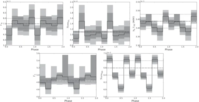
(8) The Astrophysical Journal, 808:32 (13pp), 2015 July 20. Tendulkar et al.. Table 3 NH Values From Different Abundance Models Abund.a Model aneb angr feld grsa wilm lodd aspl. NHb. Model I c2c. p-value. ± ± ± ± ± ± ±. 2725.33 2719.04 2768.78 2753.07 2826.47 2843.74 2827.83. 5.5 ´ 10-6 8.1 ´ 10-6 3.7 ´ 10-7 9.6 ´ 10-7 5.3 ´ 10-9 1.4 ´ 10-9 4.8 ´ 10-9. 1.06 0.93 0.95 1.11 1.27 1.32 1.30. 0.02 0.02 0.02 0.02 0.03 0.03 0.03. NHb. Model II c2c. ± ± ± ± ± ± ±. 2722.70 2718.96 2719.98 2719.87 2722.94 2718.83 2722.14. 0.41 0.37 0.38 0.44 0.51 0.54 0.52. 0.01 0.01 0.01 0.01 0.01 0.01 0.01. p-value. 6.5 8.1 7.6 7.7 6.4 8.2 6.7. ´ ´ ´ ´ ´ ´ ´. 10-6 10-6 10-6 10-6 10-6 10-6 10-6. NHb. Model III c2c. p-value. ± ± ± ± ± ± ±. 2553.53 2551.61 2567.20 2563.12 2588.34 2592.26 2584.44. 1.9 ´ 10-2 2.1 ´ 10-2 1.2 ´ 10-2 1.4 ´ 10-2 5.4 ´ 10-3 4.7 ´ 10-3 6.3 ´ 10-3. 0.52 0.46 0.47 0.55 0.64 0.67 0.65. 0.01 0.01 0.01 0.01 0.02 0.02 0.02. Notes. a References. aneb: Anders & Ebihara (1982), angr: Anders & Grevesse (1989), feld: Feldman (1992), grsa: Grevesse & Sauval (1998), wilm: Wilms et al. (2000), lodd: Lodders (2003), aspl: Asplund et al. (2009). b In units of 10 22 cm-2 . c Each fit has 2408 degrees of freedom.. describe the low-energy distribution. For technical reasons15, the cross-normalization factors between Swift-XRT and NuSTAR were frozen to unity. We find that Models I and II fits worsen significantly with c 2 = 5896.6 and c 2 = 3480.0 for 2413 dof respectively with extremely wavy residuals (Figure 6, Panels I and II). Model III provides a fit parameters similar to that from Table 2 with a total c 2 = 2608.3 for 2413 dof. 3.6. Phase-resolved Spectral Fits We created good-time-interval (gti) files using the measured period of 4U 0142+61 and extracted Swift-XRT and NuSTAR spectra in five equal phase bins: f = 0.0–0.2, 0.2–0.4, 0.4–0.6, 0.6–0.8 and 0.8–1.0. We fit each 0.5–79 keV spectrum with a BB+2PL and nthcomp + PL models. The fit parameters are detailed in Table 4. We froze the values of CFPMA, CFPMB and NH to those fit in the phase-averaged spectrum using the same spectral model (as in Table 2). 2 The cred for each individual phase is lower than that from the corresponding fits of the phase-averaged spectra. Figure 7 shows fit parameters for the nthcomp+PL model as a function of phase compared to the phase-averaged fit values. The spectral shape parameters GH , k B TBB and GS are statistically consistent within 3-σ with the values measured from the phaseaveraged spectra. However, we detect a very significant increase in the hard PL normalization in the 0.2–0.4 phase range which corresponds to the peak of the high-energy pulse profiles (20–35, 35–50 keV, Figure 1). Similarly, the normalization of the nthcomp component shows a sharp decrease in the 0.4–0.6 phase bin which corresponds to the dip at ϕ = 0.5 in the 3–5 and 5–8 keV pulse profiles. For the BB+2PL model, we observe a similar trend with the hard PL normalization significantly increasing in the 0.2–0.4 phase range and the soft PL normalization (which contributes approximately 85% of the X-ray flux) decreasing between the 0.4 and 0.6 phase range. In Section 3.7, we describe the variation in the high-energy spectra in greater detail with a physical emission model.. Figure 6. Data to model ratio for models fit with NH and hard power-law parameters frozen to independently measured values (see Section 3.5.2). From top to bottom, the plots represent models I, II and III.. 3.7. e Outflow Model Next we test the coronal outflow model proposed by Beloborodov (2013a). The model envisions an outflow of relativistic electron–positron (e) pairs created by electric discharge near the neutron star. The outflow moves along the magnetic field lines and gradually decelerates as it (resonantly) scatters the thermal X-rays. The outflow fills the active “jbundle” that carries the electric currents of twisted magnetospheric field lines (Beloborodov 2009). It radiates most of its kinetic energy in hard X-rays before the e pairs reach the top of the twisted magnetic loop and annihilate. The magnetic dipole moment of 4U 0142+61 is m » 1.3 ´ 1032 G cm3 (calculated from the spin-down rate; Dib & Kaspi 2014). Similar to Hascoët et al. (2014), we assume a simple geometry where the j-bundle is axisymmetric around the magnetic dipole axis. However, instead of assuming that the j-bundle emerges from a polar cap, its footprint is allowed to have a ring shape. The assumption of axisymmetry reduces the number of free parameters and appears to be sufficient to fit the phase-resolved spectra. In future work, the energy-resolved pulse profiles could be included in the fit to constrain the axial distribution of the j-bundle.. 15 Since the NH value affects only the Swift-XRT spectrum and the highenergy PL affects only the NuSTAR spectrum, allowing the cross-normalization factors to vary freely effectively allows the high-energy PL normalization to vary, spoiling the high-energy fit. To prevent this effect, we must freeze the cross-normalization constants. The expected systematic cross-calibration error between NuSTAR and Swift-XRT is approximately 5% (Madsen et al. 2015).. 8.
(9) The Astrophysical Journal, 808:32 (13pp), 2015 July 20. Tendulkar et al.. Table 4 Spectral Fits to 0.5–79 keV Phase-resolved Swift-XRT and NuSTAR Observations Component. Parameter 0.0–1.0. Phase Range 0.2–0.4 0.4–0.6. 0.0–0.2. 0.6–0.8. 0.8–1.0. const∗tbabs∗(bbody+powerlaw+powerlaw) 0.981 ± 0.015 const CFPMA 0.977 ± 0.015 CFPMB tbabs NH (10 22 cm-2 ) 1.30 ± 0.03 bbody 0.462 ± 0.005 k B TBB (keV) norma (10−3) 1.06 ± 0.04 GS powerlaw 3.85 ± 0.03 normb 0.18 ± 0.01 powerlaw 0.29 ± 0.05 GH normb (10−5) 2.3 ± 0.4 2718.6/2408 c 2 dof p-value 4.8 ´ 10-9. L L L +0.008 0.4740.008 +0.06 0.90-0.06 +0.03 3.860.03 +0.006 0.2020.007 +0.1 0.20.1 +0.8 2.10.6 1184.8/1122 9.4 ´ 10-2. L L L +0.009 0.4830.009 +0.07 1.05-0.06 +0.03 3.840.03 +0.006 0.1920.006 +0.1 0.40.1 +1.6 4.61.2 1207.4/1120 3.5 ´ 10-2. L L L +0.009 0.4670.008 +0.06 0.9880.06 +0.03 3.910.03 +0.006 0.1790.006 +0.1 0.3-0.1 +1.0 2.20.7 1011.0/1008 4.7 ´ 10-1. L L L +0.008 0.4580.008 +0.06 1.02-0.06 +0.03 3.970.03 +0.007 0.2000.007 +0.1 0.30.1 +1.0 2.60.7 1154.7/1045 9.8 ´ 10-3. L L L +0.008 0.4780.008 +0.06 0.90-0.06 +0.03 3.920.03 +0.006 0.1930.006 +0.1 0.30.1 +1.1 2.10.7 1070.2/1035 2.2 ´ 10-1. const∗tbabs∗(nthcomp+powerlaw) const 1.001 ± 0.015 CFPMA 0.998 ± 0.015 CFPMB tbabs NH (10 22 cm-2 ) 0.65 ± 0.02 nthcomp 4.86 ± 0.04 GS 0.346 ± 0.004 k B TBB (keV) k B Te- (keV) >37.3 normb (10−2) 6.5 ± 0.2 +0.05 powerlaw 0.75GH 0.04 b −4 +0.2 1.1-0.1 norm (10 ) 2550.1/2408 c 2 dof 6.3 ´ 10-3 p-value. L L L +0.06 4.810.13 +0.003 0.3440.009 >13.5 6.8 ± 0.1 +0.09 0.650.1 +0.3 0.9-0.2 1190.4/1122 7.6 ´ 10-2. L L L +0.07 4.750.30 +0.004 0.3440.006 >4.8 6.4 ± 0.1 +0.1 0.790.08 +0.6 1.4-0.3 1189.4/1120 7.3 ´ 10-2. L L L +0.08 4.890.15 +0.004 0.3400.004 >10.5 6.0 ± 0.1 +0.11 0.750.11 +0.3 1.0-0.3 1012.0/1008 4.6 ´ 10-1. L L L +0.08 4.980.22 +0.004 0.3380.004 >6.7 6.8 ± 0.1 +0.1 0.710.09 +0.3 0.9-0.2 1094.1/1045 1.4 ´ 10-1. L L L +0.10 4.940.21 +0.003 0.3460.004 >6.8 6.4 ± 0.1 +0.2 0.780.09 +0.6 1.0-0.2 1058.8/1035 3.0 ´ 10-1. Notes. a Normalization in units of L 39 D102 , where L39 is the source luminosity in units of 1039 erg s-1 and D10 is the distance to the source in units of 10 kpc. b Normalization in units of photons keV-1 cm-2 s-1 at 1 keV.. Figure 7. Variation of nthcomp+PL model parameters as a function of rotational phase. In each plot, the solid black line shows the parameter value in each phase bin, dark and light gray regions show the 1σ and 3σ error ranges respectively. The phase range is repeated twice for clarity. The dashed black line and dotted black lines show the value of the parameter in the phase-averaged spectral fit and the corresponding 3σ error bars. Starting from the top left to bottom right, the plots show GH , power law normalization, k B TBB, GS and nthcomp normalization, respectively.. 9.
(10) The Astrophysical Journal, 808:32 (13pp), 2015 July 20. Tendulkar et al.. Figure 8. Maps of p-values for the fit of the hard X-ray component with the coronal outflow model; the p-values are shown in the plane of (amag , b obs ) and maximized over the other parameters. The amag axis is common for all the plots. The p-value scale is shown on the left. The hatched green regions have p-values smaller than 0.001; the white regions have p-values greater than 0.1. Interchanging the values of amag and b obs does not change the model spectrum, as long as the j-bundle is assumed to be axisymmetric. Therefore, the map of p-values is symmetric about the line of b obs = amag . Left: p-value map when Dq j is thawed as a free parameter. Middle: p-value map when the footprint width is frozen to Dq j = q j 2. Right: p-value map when the footprint area of the j-bundle, j , is restricted to be in the interval 2.5 ´ 10-3 < j NS < 10-2 (see discussion).. This more general model has the following parameters: (1) the power L j of the e outflow along the j-bundle, (2) the angle amag between the rotation axis and the magnetic axis, (3) the angle b obs between the rotation axis and the observer’s line of sight, (4) the angular position q j of the j-bundle footprint, and (5) the angular width Dq j of the j-bundle footprint. In addition, the reference point of the rotational phase, f0 , is a free parameter, since we fit the phase-resolved spectra. We follow the method presented in Hascoët et al. (2014), and explore the whole parameter space by fitting the phaseaveraged spectrum of the total emission (pulsed+unpulsed) and phase-resolved spectra of the pulsed emission. In order to get sufficient photon statistics, we used only three phase bins: “A” (0.05–0.35), “B” (0.35–0.70), and “C” (0.70–1.05), roughly covering the primary pulse peak, the minima and the sub-peak, respectively. The bins are indicated in the last panel of Figure 1. The phase bin with the lowest flux is assumed to represent the “DC” (unpulsed) component; its spectrum is subtracted from the total spectrum in each phase bin to obtain the spectrum of the pulsed component. The NuSTAR data are fitted above 16 keV, where the hard component becomes dominant and the coronal outflow model has to account for most of the X-ray emission. The left panel of Figure 8 shows the map of p-values in the plane (amag , b obs ). The parameter space appears to be largely degenerate. For comparison with the results of Hascoët et al. (2014) (discussed further in Section 4.3 below), we also show the resulting p-value map when the footprint width is fixed to be Dq j = q j 2, i.e., thin rings are excluded. Then the degeneracy of the parameter space is significantly reduced, and the results are consistent with those of Hascoët et al. (2014). Using the obtained best-fit model for the hard X-ray component, we have investigated the remaining soft X-ray component. The procedure is similar to that in Hascoët et al. (2014): we freeze the best-fit parameters of the outflow model, and fit the spectrum in the 0.5–79 keV band including the. Swift-XRT data. As in Hascoët et al. (2014), we find that the spectrum is well fitted by the sum of one blackbody, one modified blackbody16 and the coronal outflow emission (which dominates above 10 keV). The (cold) blackbody and the (hot) modified blackbody have luminosities L c = 2.5(3) ´ 1035 erg s-1, L h = 3.33(4) ´ 1034 erg s-1 and temperatures kTc = 0.408(3) keV, kTh = 0.85(1) keV similar to those fit by model II in Section 3.5. The PL tail of the modified hot blackbody starts at Etail = 5.7(1) keV. 4. DISCUSSION AND CONCLUSION We have described timing and spectral analysis of simultaneous 0.3–79 keV Swift-XRT and NuSTAR observations of 4U 0142+61. Using Fourier analysis we present the variation in pulse shape and pulse fraction over the soft X-ray and hard X-ray bands. We find a significant change in pulse structure at the cross-over between the soft-energy peak where the modified blackbody emission is dominant and the hard-energy peak, where the magnetospheric tail emission is dominant. We do not find evidence for phase modulation in the 15–40 keV lightcurve as reported by Makishima et al. (2014). We find that the phase-averaged spectrum is best modeled by a phenomenological nthcomp+PL model. The BB+2PL and 2BB+PL models that were traditionally used to fit the data do not provide statistically acceptable descriptions. Fitting the phaseresolved Swift-XRT and NuSTAR spectra of 4U 0142+61, we find that the spectral shape parameters do not show statistically significant variations compared to the phase-averaged fits. However, the normalizations of the spectral components vary significantly at phases corresponding to peaks and dips in the pulse profiles. Finally, we place constraints on the geometry of 16 In this model, dubbed BBtail in Vogel et al. (2014), the Wien tail of the blackbody is replaced by a PL “smoothly” connected at the photon energy E tail . Here “smoothly” means that the photon spectrum and its derivative are continuous at E tail .. 10.
(11) The Astrophysical Journal, 808:32 (13pp), 2015 July 20. Tendulkar et al.. 4U 0142+61 using the electron-position outflow models of Beloborodov (2013a).. time-varying, having been detected in 2009 but not in 2007 and 2014. However, considering the necessary reconfiguration in the neutron star moments of inertia (DI I ~ 10-4 ) and the corresponding reconfiguration of a 1016 G toroidal magnetic field, it is surprising that the timing ephemeris, rotational spindown and pulse profiles remain consistent between 2007 and 2014. Further searches of phase modulation will help to confirm and understand the mechanics of this result.. 4.1. Timing Analysis The low-energy pulse shapes measured from Swift-XRT and NuSTAR agree with the measurements of dH08 gathered with XMM-Newton. In particular, the pulse profiles bear remarkable similarity with the data gathered on 2004 July 25 (dataset C) and on 2004 March 1 (dataset B) and are less similar to the previous observations (dataset A, gathered on 2003 January 04). The separation between the peaks in Swift-XRT (Df = 0.35, in 0.3–1.5 keV) matches that in the XMMNewton data (Df = 0.35, in 0.8–2.0 keV). The separation between the dips (Df = 0.6) and the relative pulse heights also match well between the two data sets. Similarly, the pulse shapes and relative heights between NuSTAR 3–5 and 5–8 keV profiles and the XMM-Newton 2–8 keV profiles are morphologically similar. Similarly, the NuSTAR 3–5 keV profile agrees with the 2–4 keV RXTE pulse profiles of Dib et al. (2007) obtained between 2005 March and 2006 February. However, there are increasing differences between the NuSTAR profile and the RXTE pulse profiles at epochs going backward from 2005 to 1996. The 6–8 keV profile between 2005 March and 2006 February shows a slightly broader main peak than the 5–8 keV NuSTAR pulse profiles. Our low-energy pulse shapes agree well with 0.5–2 and 2–10 keV XMM-Newton pulse profiles of Gonzalez et al. (2010) obtained between 2006 July and 2008 March with the match improving as the compared epochs become closer. We find slight differences between the NuSTAR 20–35 and 35–50 keV profiles and INTEGRAL20–50 keV profiles described in dH08. The NuSTAR profiles show a primary peak (at ϕ = 0.2) that is 40% higher than the secondary peak (at ϕ = 0.7). In the INTEGRAL profiles, the peak separations are similar (Df = 0.53) but the peak count rates were equal. Similarly, we find that the NuSTAR 50–79 keV profiles show evidence of a double-peaked structure, with two sharp peaks separated by Df = 0.3. The corresponding 50–160 keV INTEGRAL profile shows a single-peaked structure. While it is possible that the pulse profile has changed, note that the 50–79 keV band would contribute only 35% of the photon flux as compared to the 50–160 keV energy band for a PL spectrum with G = 0.65. Hence the difference in pulse profile may also be attributable to the difference in energy ranges. We also observe that the relative height of the primary pulse (at f » 0.3) compared to the pulse at f » 0.8 is decreasing with increasing energy through the 20–35, 35–50 and 50–79 keV plots. Hence it is not inconceivable that at energies higher than 79 keV, the pulse at f » 0.8 starts to dominate the pulse profile.. 4.1.2. Comparisons with Other Magnetars. The trend of pulse fraction as a function of energy varies from magnetar to magnetar though many have a pulse fraction increasing with energy (see for example Kuiper et al. 2006; den Hartog et al. 2008a, 2008b). In 4U 0142+61 we observe that PFrms increases up to a value of 20% and possibly shows a small decline toward 40 keV or possibly stays constant at ≈20%. In 1E 2259+596, PFrms was seen to monotonically rise to approximately 70% at 20 keV (Vogel et al. 2014) and in 1E 1841–045, PFrms was seen to rise to a value of approximately 17% at 10 keV, decrease to 12% at 20 keV and rise again to approximately 17%–20% between 30 and 79 keV (An et al. 2013; An et al. 2015, in preparation). At the same time, PFarea was measured to increase from 25% at 1–2 keV and increase to 50% at 50 keV. For 1RXS J170849–400910 (den Hartog et al. 2008a), the pulse fraction (reported as PFarea, not PFrms) was shown to be nearly constant at approximately 40% between an energy range from 0.7 to 200 keV. In fact, the pulse fraction decreases slightly from about 50% at 1 keV to about 30% at 3 keV, rising back to about 40% at higher energies. The X-ray pulse profiles of magnetars, affected by the geometry of the magnetic field and rotation axis, are similarly diverse. The pulse profiles of 4U 0142+61 are primarily double peaked for most energy bands with each pulse width being df » 0.25. Compared to these, the pulse profile of 1E 1841–045 (An et al. 2013; An et al. 2015, in preparation) is comprised of large, single-peaked humps that are about df » 0.75 wide (except for the double-peaked structure emerging between 23.8 and 35.2 keV). The pulse profiles of 1RXS J170849–400910 (den Hartog et al. 2008a) are dominated by a single pulse peak with a width df = 0.35 at most energy bands; however, there is a distinct shift between pulse positions below and above 8 keV, suggesting that the dominant emission mechanism changes drastically. The pulse profiles of 1E 2259+586 show complicated structure, with narrow peaks (df » 0.25) that can possibly shift slightly with energy (Vogel et al. 2014). The pulse profiles of 4U 0142+61 are therefore morphologically more similar to those of 1RXS J170849–400910 than those from 1E 2259+586 and 1E 1841–045. A possible source for these differences may be the size and geometry of the hot-spot emitting area on each magnetar. Comparing the size of the j-bundle, q j in the outflow model fits (see Section 4.3) suggests a rough pattern, albeit in a very limited sample size. For 1E 1841–045, the magnetar with the broadest pulse profiles, q j 0.4 rad (An et al. 2013; An et al. 2015, in preparation) while for 1RXS J170849–400910 and 4U 0142+61 with narrower pulse profiles, q j < 0.15 rad and <0.23 rad, respectively (Hascoët et al. 2014). The outflow model fit for 1E 2259+586, which shows a complicated narrow pulse profile, statistically prefers a complicated ring-shaped. 4.1.1. Non-detection of Precession. After repeating the analysis steps of Makishima et al. (2014) on 15–40 keV NuSTAR data of 4U 0142+61, we did not detect any phase modulation that can be interpreted as precession of the neutron star. The pulse profile from the NuSTAR data, while very consistent in shape and amplitude with the double-peaked profiles of dH08, are very different in shape and amplitude from the triple-peaked profiles of ME14 obtained after phasedemodulation. It is possible that the precession signal may be 11.
(12) The Astrophysical Journal, 808:32 (13pp), 2015 July 20. Tendulkar et al.. blackbody is small, h » 0.005 NS. In the coronal outflow model, the footprint of the j-bundle is expected to form a hot spot, as some particles accelerated in the j-bundle flow back to the neutron star and bombard its surface. If the modified hot blackbody is interpreted as the thermal emission from the footprint, then the measured h can be used as a constraint on the footprint of the active j-bundle. The right panel of Figure 8 shows the NuSTAR p-value when the j-bundle footprint area, is restricted to be between j = p sin2 q j , h 2 = 2.5 ´ 10-3NS and h ´ 2 = 10-2NS. Then the degeneracy of the model is reduced and a broad region of the parameter space around the line amag = b obs becomes excluded. The outflow model predicts the X-ray flux below ∼1 MeV to be dominated by photons polarized perpendicular to the magnetic field while an excess of parallel-polarized photons is expected through photon splitting at higher energies (Beloborodov 2013a). The model of magnetospheric emission will be crucially tested by future X-ray polarimetry instruments such as ASTRO-H-SGD (Tajima et al. 2010, during flares), ASTROSAT-CZTI (Chattopadhyay et al. 2014), POLAR (Produit et al. 2005) and X-Calibur (Beilicke et al. 2014). In conclusion, we have presented a timing and spectral analysis of simultaneous 0.5–79 keV observations of 4U 0142 +61 using Swift-XRT and NuSTAR. The rotational period of 4U 0142+61 is consistent with that expected from extrapolation of the timing solution since the last glitch (Dib & Kaspi 2014). We have not detected the 55 ks time period, 0.7 s amplitude phase modulation in the 15–40 keV Suzaku-HXD data from 2007 reported by Makishima et al. (2014) that was ascribed to the free-precession of 4U 0142+61. While this precession may be time-varying, the consistency of the rotational ephemeris and pulse profile between 2007 and 2014 needs to be explained. We have shown that the pulse profile changes character (dominance of the first harmonic vs the second harmonic) at around 30 keV. While the low-energy pulse profiles were consistent with previously presented pulse profiles (between 2006 and 2008: Dib et al. 2007; Gonzalez et al. 2010), we have observed morphological differences between the hard energy pulse profiles of NuSTAR and INTEGRAL. We have shown that the rms pulse fraction has an increasing trend with energy, reaching a value of up to 20%, however, it shows some evidence of a decrease at about 40 keV similar to that observed in 1E 1841–045 and contrary to the smooth increase of pulse fraction in 1E 2259+586 that increases to nearly 80%. We have shown that the energy spectrum of 4U 0142 +61 between 0.5 and 79 keV is better described by a Comptonized blackbody+hard PL model than the previously used BB+2PL or 2BB+PL models with a hard PL (GH = 0.65 0.09) dominating the spectrum above 20 keV. The low-energy spectrum (<10 keV) may still be fit with the BB+PL model, however, this model cannot fit the observed spectrum between 10 and 20 keV. We have fitted the phase-resolved spectra of 4U 0142 +61 with the e outflow model of Beloborodov (2013b) using the analysis method of Hascoët et al. (2014). Our results show that the outflow model gives a consistent physical description of the phase-resolved spectra, and the results are consistent with those derived from INTEGRAL data. We found that significant degeneracy appears in the inferred parameters of the inclined rotator amag and b obs if the footprint of the j-bundle is. j-bundle with 0.4 rad < q j < 0.75 rad and Dq j q j , the ringwidth fracion, <0.2 (Vogel et al. 2014). 4.2. Spectral Analysis We fit different spectral models to the soft and hard energy spectra from Swift-XRT and NuSTAR. We find that the 2BB +PL and BB+2PL models do not fit the cross-over region (approximately 5–15 keV) of the spectrum well. This causes a distortion in the fitting of the hard PL and a residual is left at the high energies (>50 keV). The nthcomp+PL model provides a statistically better fit than the two models, especially for the cross-over region. The hard PL index GH measured from this model best matches the GH = 0.65 0.09 measured after restricting the energy range to be between 20 and 79 keV. We find that the spectral turnover GS - GH = 3.56 (BB+2PL model) and GS - GH = 4.11 (nthcomp+PL) are higher than the values reported for the total flux GS - GH = 2.6 reported by Kaspi & Boydstun (2010). Using the independent value of GH = 0.65 0.09 slightly increases the discrepancy. Placing these values on the GS - GH versus log(B 1014 G) plot (as shown in Vogel et al. 2014), does not change the observed decreasing trend between GS - GH and log(B 1014 G). Fitting the same models to the phase-resolved spectra shows that the spectral shape parameters (GH , k B TBB and GS) are consistent within 3-σ error bars to the values measured from phase-averaged spectral fits. However, the normalization of the hard X-ray and soft X-ray components varies significantly as a function of phase. From Figure 7, we can identify the increase in the hard PL normalization in the 0.2–0.4 phase range with the peak in the 20–35 and 35–50 keV pulse profiles and the dip in the soft X-ray components normalization (nthcomp or soft PL, depending on the model fits) with the dip at phase ϕ = 0.5 in the 3–5 and 5–8 keV bands. This suggests a clear differentiation between the low-energy and high-energy spectral components. We find that the best-fitting nthcomp+PL model yields NH = (6.5 0.2) ´ 10 21 cm-2 , consistent with that measured by D06b and also consistent with later broadband fits by Enoto et al. (2011). 4.3. Outflow Model We find that the coronal outflow model provides consistent fits to the phase-resolved NuSTAR spectra of 4U 0142+61. Hascoët et al. (2014) obtained a similar conclusion by fitting the INTEGRAL phase-resolved spectra of den Hartog et al. (2008b). Their model assumed that the outflow occurs along magnetic field lines emerging from a polar cap on the star or a thick ring Dq j = q j 2. An excellent fit was provided by this model in a small region of parameter space, giving strong constraints on amag and b obs. Motivated by the recent analysis of 1E 2259+586 (Vogel et al. 2014), we explored a more general outflow model that allows the footprint of j-bundle to be a ring of arbitrary thickness Dq j . We found that a thin-ring configuration is also able to fit the phase-resolved spectrum of 4U 0142+61, and in a broader range of parameters. This degeneracy is absent in 1E 1841–045, where only a thick ring or a polar cap is allowed (An et al. 2015, in preparation). The soft X-ray component (below ∼10 keV) is well fitted by the sum of one cold blackbody and one modified hot blackbody. The cold blackbody covers a large fraction of the neutron star area, c » 0.7 NS. The emission area of the hot 12.
(13) The Astrophysical Journal, 808:32 (13pp), 2015 July 20. Tendulkar et al.. allowed to be a thin ring. The degeneracy is significantly reduced if the footprint area Aj is restricted to be similar to the area of the blackbody hotspot that covers 0.5% of the neutron star surface.. den Hartog, P. R., Hermsen, W., Kuiper, L., et al. 2006, A&A, 451, 587 den Hartog, P. R., Kuiper, L., & Hermsen, W. 2008a, A&A, 489, 263 den Hartog, P. R., Kuiper, L., Hermsen, W., et al. 2008b, A&A, 489, 245 den Hartog, P. R., Kuiper, L., Hermsen, W., & Vink, J. 2004, ATel, 293, 1 Dib, R., & Kaspi, V. M. 2014, ApJ, 784, 37 Dib, R., Kaspi, V. M., & Gavriil, F. P. 2007, ApJ, 666, 1152 Durant, M., & van Kerkwijk, M. H. 2006a, ApJ, 650, 1070 Durant, M., & van Kerkwijk, M. H. 2006b, ApJ, 650, 1082 Enoto, T., Makishima, K., Nakazawa, K., et al. 2011, PASJ, 63, 387 Enoto, T., Nakazawa, K., Makishima, K., et al. 2010, ApJL, 722, L162 Feldman, U. 1992, PhyS, 46, 202 Giacconi, R., Murray, S., Gursky, H., et al. 1972, ApJ, 178, 281 Göhler, E., Staubert, R., & Wilms, J. 2004, MmSAI, 75, 464 Göhler, E., Wilms, J., & Staubert, R. 2005, A&A, 433, 1079 Gonzalez, M. E., Dib, R., Kaspi, V. M., et al. 2010, ApJ, 716, 1345 Grevesse, N., & Sauval, A. J. 1998, SSRv, 85, 161 Harrison, F. A., Craig, W. W., Christensen, F. E., et al. 2013, ApJ, 770, 103 Hascoët, R., Beloborodov, A. M., & den Hartog, P. R. 2014, ApJL, 786, L1 Hulleman, F., van Kerkwijk, M. H., & Kulkarni, S. R. 2004, A&A, 416, 1037 Israel, G. L., Mereghetti, S., & Stella, L. 1993, IAUC, 5889, 1 Israel, G. L., Mereghetti, S., & Stella, L. 1994, ApJL, 433, L25 Israel, G. L., Oosterbroek, T., Angelini, L., et al. 1999, A&A, 346, 929 Juett, A. M., Marshall, H. L., Chakrabarty, D., & Schulz, N. S. 2002, ApJL, 568, L31 Kaspi, V. M., Archibald, R. F., Bhalerao, V., et al. 2014, ApJ, 786, 84 Kaspi, V. M., & Boydstun, K. 2010, ApJL, 710, L115 Kuiper, L., Hermsen, W., den Hartog, P. R., & Collmar, W. 2006, ApJ, 645, 556 Leahy, D. A. 1987, A&A, 180, 275 Lodders, K. 2003, ApJ, 591, 1220 Madsen, K. K., Harrison, F. A., Markwardt, C., et al. 2015, arXiv:1504.01672 Makishima, K., Enoto, T., Hiraga, J. S., et al. 2014, PhRvL, 112, 171102 Mereghetti, S. 2008, A&ARv, 15, 225 Mori, K., Gotthelf, E. V., Zhang, S., et al. 2013, ApJL, 770, L23 Olausen, S. A., & Kaspi, V. M. 2014, ApJS, 212, 6 Patel, S. K., Kouveliotou, C., Woods, P. M., et al. 2003, ApJ, 587, 367 Paul, B., Kawasaki, M., Dotani, T., & Nagase, F. 2000, ApJ, 537, 319 Predehl, P., & Schmitt, J. H. M. M. 1995, A&A, 293, 889 Produit, N., Barao, F., Deluit, S., et al. 2005, NIMPA, 550, 616 Rea, N., & Esposito, P. 2011, in High-Energy Emission from Pulsars and their Systems, ed. D. F. Torres & N. Rea (Berlin: Springer), 247 Rea, N., Esposito, P., Turolla, R., et al. 2010, Sci, 330, 944 Rea, N., Nichelli, E., Israel, G. L., et al. 2007, MNRAS, 381, 293 Scholz, P., Kaspi, V. M., & Cumming, A. 2014, ApJ, 786, 62 Tajima, H., Blandford, R., Enoto, T., et al. 2010, Proc. SPIE, 7732, 16 Thompson, C., & Duncan, R. C. 1995, MNRAS, 275, 255 Thompson, C., & Duncan, R. C. 1996, ApJ, 473, 322 Thompson, C., Lyutikov, M., & Kulkarni, S. R. 2002, ApJ, 574, 332 Vogel, J. K., Hascoët, R., Kaspi, V. M., et al. 2014, ApJ, 789, 75 White, N. E., Angelini, L., Ebisawa, K., Tanaka, Y., & Ghosh, P. 1996, ApJL, 463, L83 Wilms, J., Allen, A., & McCray, R. 2000, ApJ, 542, 914 Yan, M., Sadeghpour, H. R., & Dalgarno, A. 1998, ApJ, 496, 1044 Życki, P. T., Done, C., & Smith, D. A. 1999, MNRAS, 309, 561. This work was supported under NASA Contract No. NNG08FD60C, and made use of data from the NuSTAR mission, a project led by the California Institute of Technology, managed by the Jet Propulsion Laboratory, and funded by the National Aeronautics and Space Administration. We thank the NuSTAR Operations, Software and Calibration teams for support with the execution and analysis of these observations. This research has made use of the NuSTAR Data Analysis Software (NuSTARDAS) jointly developed by the ASI Science Data Center (ASDC, Italy) and the California Institute of Technology (USA). V. M. K. acknowledges support from an NSERC Discovery Grant and Accelerator Supplement, the FQRNT Centre de Recherche Astrophysique du Québec, an R. Howard Webster Foundation Fellowship from the Canadian Institute for Advanced Research (CIFAR), the Canada Research Chairs Program and the Lorne Trottier Chair in Astrophysics and Cosmology. A.M.B. acknowledges the support by NASA grant NNX13AI34G. REFERENCES An, H., Archibald, A. M., Hascoet, R., et al. 2015, arXiv:1505.03570 An, H., Hascoët, R., Kaspi, V. M., et al. 2013, ApJ, 779, 163 An, H., Kaspi, V. M., Archibald, R., et al. 2014a, AN, 335, 280 An, H., Kaspi, V. M., Beloborodov, A. M., et al. 2014b, ApJ, 790, 60 Anders, E., & Ebihara, M. 1982, GeCoA, 46, 2363 Anders, E., & Grevesse, N. 1989, GeCoA, 53, 197 Arnaud, K. A. 1996, in ASP Conf. Ser. 101, Astronomical Data Analysis Software and Systems V, ed. G. H. Jacoby & J. Barnes (San Francisco, CA: ASP), 17 Asplund, M., Grevesse, N., & Sauval, A. J. 2005, in ASP Conf. Ser. 336, Cosmic Abundances as Records of Stellar Evolution and Nucleosynthesis, ed. T. G. Barnes, III & F. N. Bash (San Francisco, CA: ASP), 25 Asplund, M., Grevesse, N., Sauval, A. J., & Scott, P. 2009, ARA&A, 47, 481 Balucinska-Church, M., & McCammon, D. 1992, ApJ, 400, 699 Beilicke, M., Kislat, F., Zajczyk, A., et al. 2014, JAI, 3, 40008 Beloborodov, A. M. 2009, ApJ, 703, 1044 Beloborodov, A. M. 2013a, ApJ, 777, 114 Beloborodov, A. M. 2013b, ApJ, 762, 13 Brazier, K. T. S. 1994, MNRAS, 268, 709 Burrows, D. N., Hill, J. E., Nousek, J. A., et al. 2005, SSRv, 120, 165 Chattopadhyay, T., Vadawale, S. V., Rao, A. R., Sreekumar, S., & Bhattacharya, D. 2014, ExA, 37, 555. 13.
(14)
Figure


+5


Documento similar
