The Next Generation Virgo Cluster Survey (NGVS) XXXII A Search for Globular Cluster Substructures in the Virgo Galaxy Cluster Core
11
0
0
Texto completo
(2) The Astrophysical Journal, 856:84 (11pp), 2018 March 20. Powalka et al.. stellar population properties (Powalka et al. 2016a), and a more complete usage of the SED may allow us to unravel more details of GC assembly histories. In the earlier articles of this series (Powalka et al. 2016a, 2017, hereafter referred to as Papers I and II), we studied the GCs in the Virgo core region (around M87) using the data of the Next Generation Virgo Cluster Survey (NGVS/NGVS-IR; see Ferrarese et al. 2012; Muñoz et al. 2014). We confronted their u*, g, r, i, z, Ks photometry with the predictions of single stellar population (SSP) models for a broad grid of ages and metallicities. Although the absolute ages and metallicities one may assign to the GCs are affected by biases and should be manipulated with great caution, we emphasized that the relative values of these assigned labels contain rich information on the relative positions of the GCs in color space, and may be sensitive to subtle differences such as those induced by modified abundance ratios. Therefore, in this paper we analyze the spectral energy distributions (SEDs) of Virgo core GCs using derived quantities (mainly formal labels of age and metallicity) from our broadband photometric filter set. Knowing that the cD galaxy M87 has experienced multiple mergers, we aim to search for local variations that might indicate differences in GC origins.. Table 1 Stellar Libraries and Isochrone References for the Different SSP Models Used in This Paper Model. Stellar Librarya. Isochrones. BC03 BC03B C09BB C09PB C09PM M05 MS11 PEG PAD VM12. STELIB BaSeL 3.1 BaSeL 3.1 BaSeL 3.1 MILES BaSeL 3.1 MILES BaSeL 2.2 ATLAS ODFNEW/PHOENIX BT-Settl MILESb. Padova 1994 Padova 1994 BaSTI Padova 2007 Padova 2007 Cassisi Cassisi Padova 1994 PARSEC 1.2S Padova 2000. Notes.Models:BC03 and BC03B—Bruzual & Charlot (2003). C09BB, C09PB and C09PM—(FSPS v2.6) Conroy et al. (2009). M05 and MS11— Maraston (2005), Maraston & Strömbäck (2011). PEG—Fioc & RoccaVolmerange (1997). PAD—CMD v2.8 (see footnotehttp://stev.oapd.inaf.it/ cgi-bin/cmd). VM12—Vazdekis et al. (2012), Ricciardelli et al. (2012). Libraries and isochrones: ATLAS ODFNEW refers to Castelli & Kurucz (2004). BaSeL: Lejeune et al. (1997, 1998), Westera et al. (2002). BaSTI: Pietrinferni et al. (2004), Cordier et al. (2007). Cassisi: Cassisi et al. (1997a, 1997b, 2000). MILES: Sánchez-Blázquez et al. (2006). Padova 1994: Alongi et al. (1993), Bressan et al. (1993), Fagotto et al. (1994a, 1994b), Girardi et al. (1996). Padova 2007: Girardi et al. (2000), Marigo & Girardi (2007), Marigo et al. (2008). PARSEC 1.2S: Bressan et al. (2012), Tang et al. (2014), Chen et al. (2014, 2015). PHOENIX BT-Settl: Allard et al. (2003). STELIB: Le Borgne et al. (2003). a Optical-only libraries are generally combined with BaSeL at UV and IR wavelengths in the original codes. b The MILES library extends from 3464 to 7500 Å. In order to reach u*, i, and z magnitudes, we used the combination of NGSL and MIUSCAT from Koleva & Vazdekis (2012; they provide wavelengths from ∼1700 to ∼9500 Å) and we extrapolated the NGSL+MILES+MIUSCAT spectra from 9500 to 10000 Å using Pegase GC spectra.. 2. The Data: Next Generation Virgo Survey GCs 2.1. Colors and Magnitudes In this paper, we use the high-quality aperture-corrected photometry of the Virgo GC sample defined in Paper I.17 This data set consists of 1846 GCs located within a 3.62 deg2 field of view around M87 with photometry in u*, g, r, i, z from CFHT/MegaCam (Boulade et al. 2003).18 The SExtractor19 magnitude random errors in this sample are smaller than 0.06 mag in each band and a budget of systematic errors including errors on calibration, extinction, and filter transmission is presented in Paper I. The GC sample contains predominantly bright Virgo GCs with mean magnitudes of approximately 23.05, 21.88, 21.32, 21.05, 20.87 in the u*, g, r, i, z filters, respectively.These magnitudes correspond to typical GC masses of about 2×10⁶ Me at the distance of M87.. a GC with a SSP with solar-scaled metal abundances, the model-dependence of predicted colors, and the age–metallicity degeneracy, are among the main issues known to affect the final estimates.Paper II emphasized how delicate it is to estimate an absolute value of age and metallicity accurately. Therefore, in this letter, we restrict ourselves to the usage of the relative age and metallicity scale, which is a surrogate of the relative position of each GC in a multi-dimensional color space. Following the analysis in Paper II, we derive for each GC three different CEs of the age and metallicity labels, based on three different subsets of SSP models that are designed to let us search for any dependence of our analysis on the models’ input stellar spectral libraries.We recall the full list of models in Table 1. The first set (SET1) contains three SSP models based on the MILES library for the optical wavelengths (C09PM, MS11, VM12). The second one (SET2) includes seven models based on the BaSeL, STELIB, and ATLAS libraries (BC03, BC03B, C09BB, C09PB, M05, PAD, PEG). Finally, the third one (SET3) groups all 10 models. We use these three sets to search for inhomogeneities in the spatial distribution of the GC SEDs, which could be signatures of events in the galaxy’s past.. 2.2. Relative Ages and Metallicities In Paper II, we focused on estimating photometric ages and metallicities for the selected Virgo GCs.We conducted that study by comparing theoretical colors from 10 SSP models available in the literature with our observed GC colors. For any given set of SSP model grids (the 10 just mentioned or subsets thereof), we designed a “concordance estimate” (CE) to assign formal age and metallicity labels to GCs. Those labels extend from 1 to 14 Gyr for the ages and from −2.0 to 0.17 for the metallicity ([Fe/H]). The CE is defined as the photometric age and metallicity on which those models tend to agree when each of them is used in a simple maximum likelihood analysis (see Paper II for the precise definition of the adopted robust weighting scheme). In practice, the resulting values are sensitive to several systematic effects. The approximation of 17. http://vizier.u-strasbg.fr/viz-bin/VizieR?-source=J/ApJS/227/12 We will not use the Ks photometry here because of its larger random photometric errors. 19 Bertin & Arnouts (1996).. 2.3. Stellar Color Homogeneity. 18. The photometric calibration of the NGVS data relies on point sources common to NGVS and to the Sloan Digital Sky Survey 2.
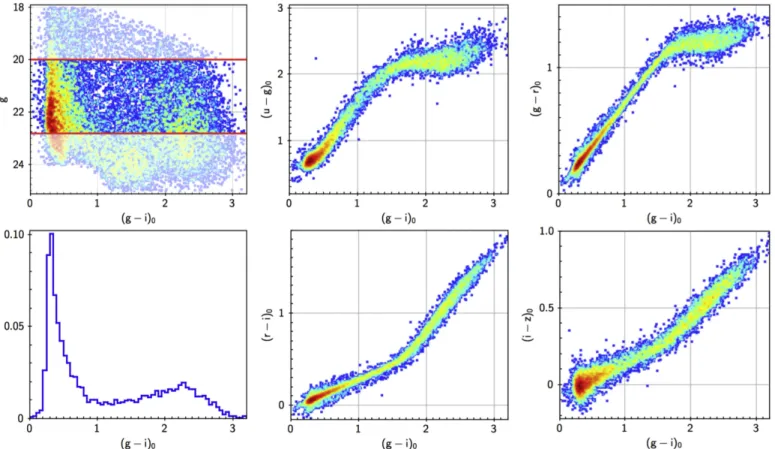
(3) The Astrophysical Journal, 856:84 (11pp), 2018 March 20. Powalka et al.. Figure 1. Star selection for the study of the homogeneity of the photometry. Stars with (g−i)0<0.6 are mostly turnoff stars of the Milky Way halo, more specifically of the Virgo Overdensity and the Sagittarius stream (Jerjen et al. 2013; Durrell et al. 2014; Lokhorst et al. 2016), while red stars are mostly the fainter dwarfs of the Milky Way disks. Among the stars in the first panel, we select those with 20<(g−i)0<22.8. The color–color diagrams and the (g−i)0 histogram for the selected subset are shown in the subsequent panels (a handful of outliers seen in those diagrams are removed for the analysis).. (SDSS). The magnitude range of overlap between these two surveys limits the number of such sources, and hence also the spatial scale on which local deviations between the surveys may be evaluated.To assess the internal homogeneity of the photometry more precisely, we investigate the distribution of stellar colors within the NGVS pilot field using a larger and deeper stellar sample, this time without the restriction of requiring good SDSS photometry.We select the stars for this procedure using the uiKs color–color diagram (Muñoz et al. 2014) together with a measure of source compactness (the latter helps with excluding Virgo GCs, as described in Paper I). The top left panel of Figure 1 illustrates the color–magnitude diagram of the initial stellar sample, restricted to 18<g<25 mag to avoid saturation and to limit photometric errors.Because the survey depth is not uniform in all the photometric bands that define the completeness of this initial catalog, we further restrict the sample everywhere to 20<g<22.8 mag.This conveniently removes the magnitude range in which the separation between stars and GCs remains difficult even with the uiKs-based method (g>23, and 0.5<(g−i)0<0.9).The cut at g=22.8 also avoids a magnitude range where the peak of the main sequence color distribution moves to redder values.The properties of the subset are shown in the remaining panels of Figure 1.We then produce R.A.–decl. maps of the difference, Δ, between the local average color and the global average. To limit the errors on the estimated local mean, we restrict our sample again, focusing on the peak of the color distribution: (g−i)0<0.5 mag. This cut is wide enough to avoid edge effects, since errors on individual star colors are of a. few percent at most, and errors on the local systematics (as we shall see) as well. Changes of ±0.1 in the color-cut do not modify the results, but the significance with which departures of Δ from 0 can be estimated drops if the color-range kept is much larger. The local average is estimated within a circle of 0°. 2 radius, which ensures each estimate is based on 80–150 stars except in field corners. The R.A.–decl. maps of the error on the local mean, σΔ, are mostly flat, with typical values summarized in Table 2. Figure 2 shows the local color deviations, Δ, at the locations of GCs. The highest correction values are observed in the (u−g) and (i−z) maps with amplitudes between −0.04 and 0.06 mag.The other colors, (g−r) and (r−i), are less affected by the correction, with amplitudes between −0.02 and 0.02 mag.We observe that the patterns in the (u−g), (g−r), and (i−z) correction maps are independent.There is some level of anti-correlation between the patterns in (g−r) and (r−i), but the two maps combined provide a map of (g−i) deviations that is not flat and that has a morphology more similar to the (g−r)-map than to the (r−i)-map. The departures of Δ from 0 are significant at the 2σΔ level over 25% to 40% of the field, except in (i−z)0, where the significant deviations cover about 80% of the observed area.This level of significance was assessed in two ways. First, we computed the ratio of Δ to the uncertainties of that estimated local mean σΔ (standard deviation in the color/root of the local sample size).Second, we applied a Kolmogorov– Smirnov (KS) test to local color distributions.With our selection cuts, we found excellent agreement between regions 3.
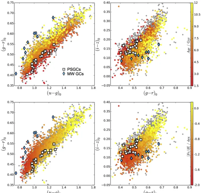
(4) The Astrophysical Journal, 856:84 (11pp), 2018 March 20. Powalka et al.. ellipses centered on M87, with radially dependent ellipticities and position angles in agreement with values from Durrell et al. (2014) and Janowiecki et al. (2010), we find that a randomly selected subset of 20% of the GCs, at the location of the feature of interest and in an area of the same size (i.e., a circular patch of 20 +2 0°. 1 diameter), should contain L = 51 objects on average. The area of the feature we are observing contains approximately 20 GCs21 of sample , which is again a significant excess (more than 6σ when using Poisson statistics for Λ=5, and still more than 4σ if Λ=7).Surprisingly, as shown in Figure 5, we do not find any large Virgo galaxy in this area, which could potentially host this accumulation of GCs.In the left and middle panels of Figure 4, we confirm that the area is mainly composed of GCs that are members of group , unlike its surroundings, which are principally occupied by GCs belonging to group . These observations hint at a possible GC substructure, with a 4D position in color space different from those of the neighboring GCs in the (projected) spatial distribution. Another similar feature is seen to the northwest of M87, around R.A.=187.45 and decl.=12.55. It has a lower contrast in Figure 3 (left panels) than the Southern feature, but is conspicuous in Figure 4. Because it is located in the region of overlap of the corners of the four individual fields of view that were combined to cover the area of our study (see, e.g., Figure 4 in Ferrarese et al. 2012), its photometry is more uncertain even after our corrections. As a result, the significance of the difference in CE ages between this particular region and its surroundings is low. Finally, in the right panels of Figure 4, we note a few patches with enhanced proportions of GCs of group . These regions are difficult to study further because they represent very small numbers of GCs. Some are associated with galaxies, such as M86 or NGC 4438, and hence are not the types of features we are for. In this paper we focus on the overdensity to the south of M87 because it has the strongest level of significance.Within this region, ∼20 GCs belong to group , with photometrically computed stellar masses (0.4 - 3) · 106 M.Hereafter, these 20 GCs are labeled PSGCs (Potential Substructure GCs).In Figure 6, we look at their color–color distributions in the context of the full GC sample. We color-code the symbols with the age and metallicity results from our CE.The top and bottom panels are, respectively, color-coded by the CE age and metallicity derived with SET1 models.In each case, both the (u−g)0 versus(g−r)0 and the (g−r)0 versus(i−z)0 color–color diagrams are plotted. PSGCs are highlighted with white squares and we additionally show a sample of Milky Way GCs (defined in Powalka et al. 2016b) with blue diamonds. In both color–color diagrams, we observe that the sequence of the PSGCs is tighter than the full GC sample. Although the gradients of photometric CE age and metallicity have a weak meaning, the PSGC locus seems to follow a relatively young iso-age region in both color–color diagrams, and to be consistent with a range of relatively low metallicities. Their location supports the fact that the overdensity observed in Figures 3 and 4 has its cause in the combination of the spatial clustering and the 4D color space age coherence. In Powalka. Table 2 Error on the Local Mean Color, in Magnitude, for the Star Subset Defined in the Text. σΔ. (u−g)0. (g−r)0. (r−i)0. (g−i)0. (i−z)0. 0.012. 0.007. 0.007. 0.008. 0.006. Note. These values may be exceeded along the edges of the field.. where Δ differs from 0 to more than 2σΔ, and regions where the assumption of identical global and local color distributions can be rejected at the 95% confidence level via the KS-test. There are several possible causes for the local deviations from the global color distributions. Subsequently, we assume that zero-point errors are dominant. Hence, we can use the Δmaps (see Figure 2) as a correction to enforce uniform photometry. We will return to the discussion of this assumption in Section 4. In the following, the relative GC ages are estimated after the inclusion of the above correction in the four colors used, i.e., (u−g)0, (g−r)0, (r−i)0, and (i−z)0. 3. Results For each of the model sets, as defined in Section 2.2 (SET1 to SET3), we divide our GC sample into three groups based on the relative formal ages assigned by our CE labeling method.The first one ( ) comprises the 20% of GCs with the youngest age labels.The second group ( ) contains the intermediate-age GCs (60% of the GC sample for each set) and the last one ( ) takes the 20% of GCs ranked as the oldest. Figure 3 illustrates the spatial distribution of each GC sample , , and , as obtained with each of the three SSP model sets.The color-code displays the local density of GCs, derived with a Gaussian kernel density estimator, with the same bandwidth in each of the nine panels. Note that the distributions from SET1, SET2, or SET3 are highly consistent with each other for each age group , , and .Although each set gives slightly different absolute ages (see also Paper II), we observe the same relative features independently of the model set.This emphasizes that what we call the “relative age label” only probes the relative position of any GC in the 4D color space, which does not strongly depend on the set of models.Not surprisingly, we find in each panel an overdensity of GCs concentrated around M87, a small region that contains about 50% of our GC sample.It is clearly visible at the center of the distribution in each panel.As the GC distribution is not uniform but exhibits a centrally concentrated number density profile, we additionally present in Figure 4 an alternative color-coding defined by the ratio of the sub-sample density (, , or ) by the full sample density ( + + ). This plot represents the proportion of GCs in each of the , , or samples relative to the full distribution, and can be used to identify candidate regions with an excess of clusters of one or the other category. Looking at sample in Figures 3 and 4, we note an overdensity of GCs belonging to group , in the south of M87, and centered at R.A.=187.7 and decl.=+12.2 and highlighted by a black dashed rectangle.The absolute difference between the mean CE age at this location and the mean in the surroundings equals five to seven times the standard deviation among the surrounding CE ages (depending on the set of models used), which makes it highly significant.When counting GCs in. 20. To avoid underestimating the radial number density profile, we re-inject star clusters with poorer r-band photometry into the sample; these are present at detector-chip boundaries in one of the quadrants of the Virgo core observations, as described in Paper I. 21 There is a small systematic uncertainty of about ±1 GC, which is due to variations resulting from (1) the particular set of SPS models used to compute the ages, and (2) the correction maps using the stellar colors.. 4.
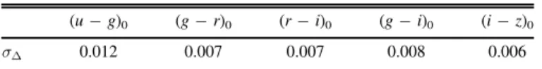
(5) The Astrophysical Journal, 856:84 (11pp), 2018 March 20. Powalka et al.. Figure 2. GC spatial distribution, color-coded by the stellar color homogeneity correction detailed in Section 2.3; the symbol colors map the offsets between local and global average stellar color, for the color index given in the bottom right corner of each panel.The black dashed rectangle highlights the position of the potential GC substructure discussed in Section 3 and later. The black star shows the location of M87, close to the center of the Virgo cluster.. et al. (2016b) we had already noted that bright Virgo GCs with colors more similar to those of MW GCs, and correspondingly older age labels according to our CEs, are not spatially concentrated but spread over the whole area of the Virgo core field discussed here.. to explain anomalies in the spatial distributions of GC colors as data reduction artifacts. While some low-significance substructure in the GC color-maps was eliminated in this process, the candidate substructure that is the focus of this paper could not be erased. Our local photometry corrections assume that the spatial patterns in Figure 3 are predominantly due to local zeropoint errors. Here, we examine alternative origins, such as selection effects in the star catalogs, real patterns in the stellar colors, local measurement errors due to the presence of extended galaxies, extinction, or the high sensitivity of CE ages to small changes in color in specific parts of the SED.. 4. Discussion Using CE age labels to characterize the broadband energy distributions of GCs, and looking at the spatial distribution of those labels around M87, we found a relatively small area to the south of M87 (∼0.1 deg2), where a concentration of GCs consistently exhibits photometric properties different from the GCs in the surroundings. This is an intriguing result, and we start this discussion by re-examining the significance of this detection. We then consider the origins such a feature may have, if confirmed by future observations.. 4.1.1. Selection Effects. The depth of the NGVS+NGVS-IR surveys is not uniform over the field of the Virgo core (especially in Ks, which is used for the separation of stars from GCs; Muñoz et al. 2014).By carefully selecting a range of stellar magnitudes and colors when calculating the maps of Section 2.3, we have limited the risk that the patterns may come from spatially varying selection effects. Failing to apply clean bright and faint magnitude cuts, or to focus on the peak of the (g−i)0 color distribution, produces maps for Δ with spatial patterns that are independent of color (except for [i−z], which remains a special case), showing that selection effects are dominant. For local zeropoint errors, we do not expect spatial correlations between. 4.1. Significance of the GC Substructure Detection The possible substructure south of M87 was first detected in the spatial maps of the CE ages obtained with the original photometry of Paper I, i.e., before the local photometric corrections of Section 2.3. In fact, the analysis of the homogeneity of stellar colors and the resulting local photometric spatial uniformity corrections were part of our attempts 5.
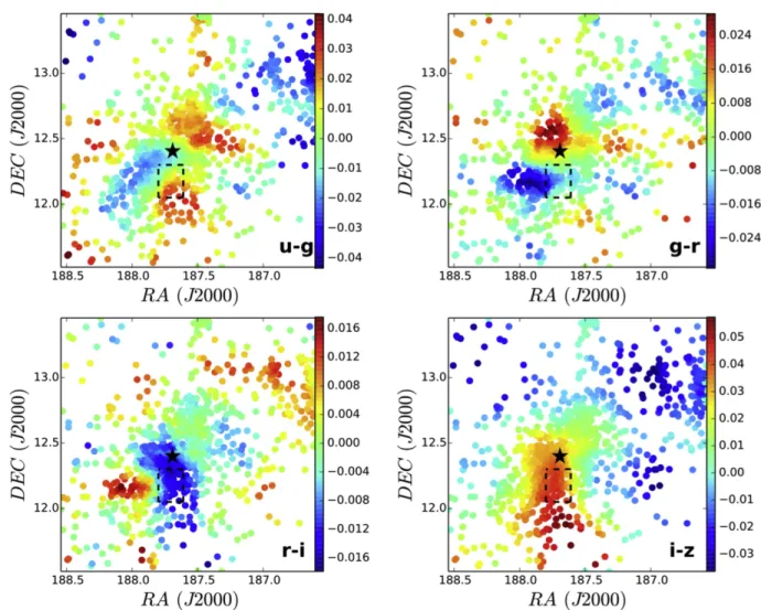
(6) The Astrophysical Journal, 856:84 (11pp), 2018 March 20. Powalka et al.. Figure 3. Spatial distributions of our sample GCs after separation into three relative age groups (columns for groups , , and , with containing the 20% that are formally the youngest GCs, containing the 20% that are formally the oldest ones, and containing the remaining 60% ), while each row of the figure is associated with a different set of SSP models.SET1 contains three SSP models based on the MILES library, SET2 contains seven models based on the BaSeL, STELIB, and ATLAS libraries, and SET3 groups all 10 models presented in Table 1 (see Section 2.2 for details). We recall that the formal ages, derived from comparisons between observed colors and SSP models, are not used for their absolute value but only as a particular way of summarizing the positions of GCs relative to the typical model locations in color space. The display color is related to the local density of GCs, as estimated with a kernel density estimator (the same kernel is used in all panels). Blue colors indicate low density, while red colors mark high-density regions. The black dashed rectangle south of M87 shows a region containing a relatively dense accumulation of younger GCs. We also point out the central disky alignment of GCs belonging to group that are symmetrically distributed around the M87 core. This structure is aligned with the large-scale GC distribution.. stellar color-correction maps that have no passband in common. The cuts we have applied mostly remove any such spatial correlation between independent color-corrections, while keeping a sample large enough to avoid strong edge effects and insufficient statistics. We have already mentioned that changing the exact position of the color and magnitude cuts does not affect the Δ-maps significantly. In particular, we found that removing the objects bluer than the typical turnoff, e.g., with (g−i)0<0.15, was not critical. We also found that the significance of the features in the Δ-maps drops when stars with a much broader range of colors, or alternatively only red stars, are kept in the sample (which is expected, considering the shape of the color distribution in Figure 1). Unfortunately, the significance also drops when the radii in which the local estimates of Δ are computed is reduced below 0°. 2, because of insufficient statistics. This remains a limitation of our corrections, although instrumental causes for variations on such small scales are few (remnant effects of gaps between detector chips and individual fields are the main ones we are aware of).. 4.1.2. Real Patterns in the Stellar Colors. The line of sight toward the core of Virgo crosses the Milky Way halo in the direction of the Virgo Stellar Overdensity (VSO) and of a major stream of the Sagittarius dwarf galaxy (Jerjen et al. 2013; Durrell et al. 2014; Lokhorst et al. 2016). In the range of g-band magnitudes we have selected, bright blue stars are thought to belong mostly to the VSO, while fainter ones belong to the Sagittarius stream.Because the stream and VSO may have spatial substructure, their relative proportions may vary locally and produce differences in Δ that should not be artificially removed. However, the average colors of bright and faint stars in our star sample differ by less than 0.008 mag (in all colors used), which is negligible for our study (and is not measurable locally). 4.1.3. Local Artifacts Due to Extended Galaxies. The photometry of stars and GCs is sensitive to local background subtraction, in particular near galaxies. We assessed this using two NGVS source catalogs, one of which 6.
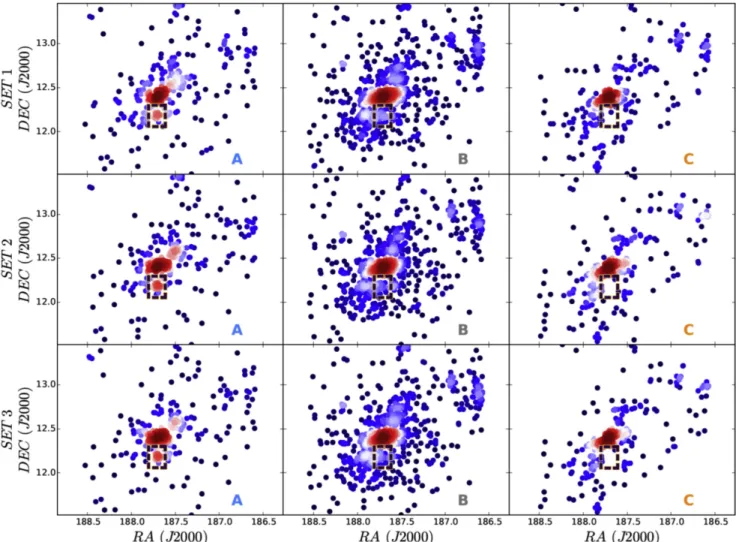
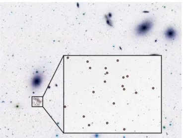
(7) The Astrophysical Journal, 856:84 (11pp), 2018 March 20. Powalka et al.. Figure 4. The same GC spatial distributions as in Figure 3, except the colors of the symbols encode the local fraction of the number of GCs of one group (, , or ) to the total number of GCs ( + + ). Red areas represent high fractions, and blue areas represent low fractions.. of galaxies. However, no such changes are found near the feature we are studying here. 4.1.4. Extinction. The dereddening of the GC photometry is based on the extinction map of Schlegel et al. (1998), as described in Paper I.The average extinction value along the line of sight toward M87 is small, i.e., áE(B - V )ñ = 0.024 mag. In both the Schlafly & Finkbeiner (2011) and the Schlegel et al. (1998) extinction maps, we observe that the NGVS central field is located in a line of sight unobscured by dust clouds. The closest cirrus is located ∼1° south of M87, whereas the PSGCs are centered about 0°. 2 off M87 in the same direction. This result is also confirmed in studies of intra-cluster light in the Virgo core region by Rudick et al. (2010). However, as a sanity check, we have assessed the effect of artificially strengthening or weakening the extinction along the line of sight toward the PSGCs. We repeated our complete analysis with 3×more and 3×less extinction in these directions. When multiplying the extinction by a factor 3, we only observe a mean age and metallicity variation of 0.3 Gyr and 0.018 dex, respectively. When dividing by the same factor, these variations reach 0.10 Gyr and 0.03 dex. In both cases, the PSGCs remain different from their neighbor GCs, thus none of our conclusions are modified.. Figure 5. Spatial distribution of the potential substructure GCS. The PSGCs (brown circles) are displayed on an NGVS image in the zoomed-in panel.The background image is taken from the Sloan Digital Sky Survey (SDSS). The three large elliptical galaxies seen in this image are, from left to right (i.e., from east to west), M87, M86, and M84. The zoomed-in inset covers an area of 6 7×5 1 (corresponding to 32.2×24.5 kpc2).. contains measurements made after galaxy subtraction (as in Alamo-Martínez & Blakeslee 2017). Indeed, colors may vary by up to 0.02 mag in regions of ∼0°. 1 diameter at the location 7.
(8) The Astrophysical Journal, 856:84 (11pp), 2018 March 20. Powalka et al.. Figure 6. Color–color diagrams for the full NGVS GC sample used in this study. Top panels: (u−g)0 vs.(g−r)0 (left) and (g−r)0 vs.(i−z)0 color–color diagram (right), where the symbol colors encode the concordance estimates of ages (see color scale on the right). The white squares mark the PSGC members of group , located in the southeast of M87 and discussed in Section 3. The blue diamonds refer to the Milky Way GCs presented in Powalka et al. (2016b). The gray points show the colors of the NGVS GCs before the correction of Section 2.3.Bottom panels: same as the the top panels, but the symbol color is parameterized by the concordance estimates of [Fe/H](see the color scale on the right).. accretions, and that these events have added numerous preexisting or newly formed GCs to the progenitor (e.g., Côté et al. 1998; Beasley et al. 2002; Hartwick 2009; Renaud & Gieles 2013). In a recent study, Ferrarese et al. (2016) estimated that as many as 40% of the current M87 GCs could come from disrupted satellites.This large number lends support to the idea that, within M87, we should observe GCs of various origins, potentially with significantly different chemodynamical properties. It is worthwhile to examine whether the GC substructure discovered in this work could belong to the remnant GC system of a disrupted galaxy.. 4.1.5. Sensitivity of CE Estimates to Small Errors in Colors. Finally, we recall that the transformation from a set of four colors to an age label is a highly nonlinear process.We tested that small systematic changes in the particular colors of the PSGCs do not lead to large changes in the the age labels. The changes applied were vectors in 4D color space whose four coordinates took values of −2, −1, 1, or 2×σΔ (all possible combinations). The feature in relative age maps is robust with respect to such changes: in all cases, the difference between the average age label within the feature and the average age label around is more than five times the statistical uncertainty on this difference. 4.2. An Astrophysical Origin of the GC Substructure?. 4.2.1. Previously Described Candidate Substructures in the M87 Halo. The dominant galaxy formation scenarios suggest that M87, like other cD galaxies, has grown through multiple mergers and. Previous searches for structure around M87 (other than deep imaging of the diffuse light) have exploited kinematical 8.
(9) The Astrophysical Journal, 856:84 (11pp), 2018 March 20. Powalka et al.. Table 3 Colors and Known Radial Velocities for the PSGCs R.A.. Decl.. gmag. (u*−g)o. (g−r)o. 187.710 187.657 187.676 187.696 187.691 187.708 187.690 187.728 187.729 187.726 187.754 187.708 187.751 187.689 187.685 187.700 187.689 187.734 187.710 187.723. 12.210 12.188 12.183 12.218 12.190 12.205 12.199 12.146 12.217 12.210 12.167 12.148 12.221 12.141 12.200 12.170 12.186 12.156 12.194 12.183. 20.99 21.80 21.61 21.92 22.11 22.32 21.60 21.91 21.99 20.98 21.65 22.30 22.33 20.97 21.96 21.90 21.85 22.59 21.93 20.65. 1.033 0.996 1.107 0.916 1.007 1.144 1.24 0.991 1.295 0.981 1.151 1.049 1.502 1.023 1.21 1.174 1.167 1.43 1.022 1.127. 0.454 0.413 0.48 0.393 0.425 0.496 0.505 0.404 0.508 0.427 0.479 0.451 0.581 0.461 0.494 0.507 0.505 0.57 0.455 0.476. (r−i)o (i−z)o as in Paper I 0.165 0.205 0.208 0.166 0.205 0.201 0.233 0.205 0.288 0.189 0.228 0.179 0.321 0.174 0.234 0.203 0.213 0.293 0.186 0.214. 0.184 0.202 0.199 0.172 0.172 0.232 0.236 0.153 0.236 0.166 0.185 0.174 0.246 0.172 0.206 0.221 0.197 0.232 0.174 0.169. (i−Ks)o. (u*−g)o. −0.101 −0.071 0.084 −0.208 −0.085 0.225 0.175 −0.175 0.228 −0.181 0.069 −0.004 0.395 −0.098 0.108 0.169 0.109 0.316 −0.072 0.021. 1.023 0.978 1.087 0.905 0.990 1.133 1.225 0.969 1.287 0.972 1.139 1.021 1.500 0.997 1.194 1.150 1.148 1.410 1.008 1.112. (g−r)o (r−i)o (i−z)o after recalibration 0.470 0.423 0.490 0.405 0.437 0.512 0.518 0.415 0.522 0.443 0.498 0.459 0.597 0.470 0.506 0.517 0.516 0.584 0.469 0.491. 0.178 0.219 0.222 0.179 0.218 0.215 0.246 0.215 0.300 0.202 0.235 0.190 0.331 0.187 0.247 0.216 0.226 0.302 0.199 0.225. 0.142 0.167 0.160 0.131 0.131 0.190 0.195 0.107 0.191 0.122 0.141 0.127 0.203 0.127 0.166 0.176 0.155 0.187 0.131 0.124. (i−Ks)o. VEL (km s−1). −0.095 −0.062 0.089 −0.208 −0.083 0.232 0.178 −0.172 0.233 −0.175 0.074 −0.003 0.400 −0.092 0.112 0.170 0.111 0.320 −0.067 0.023. 1390a 747a L L L L L L L 778b L L L 1156b 1419a L L L L 1550b. Notes. a Strader et al. (2011). These three objects are also known as [SRB2011] H25523, [SRB2011] H23419, [SRB2011] H24651. b Spectra obtained by E. W. P. et al. at the MMT Observatory, Mt. Hopkins, Arizona.. properties, although these are expensive to obtain. Romanowsky et al. (2012) used the radial velocities of about 800 GCs and searched for wedge-shaped features in phase space (radial velocity versus distance to M87) as a signature of coaccreted GC populations. They identified one candidate structure, for which they excluded chance detection in a random distribution at the 99% level.In projection on the sky, the GCs in that structure trace a flattened ring-like feature around M87, a shape consistent with the idea of a tidaldisruption event of an infalling satellite galaxy. Our analysis method could not have detected a population so broadly spread out. The (g−i) colors and spectroscopic metallicity-indicators reported by Romanowsky et al. (2012) for the GCs associated with the “wedge” (when available) suggest a broad range of chemical properties, which does not exclude, but also does not provide, extra support for the accretion picture. Another candidate structure was reported by Longobardi et al. (2015), based on the radial velocities and positions of planetary nebulae (PNe) around M87. Bright PNe are associated with the final stellar evolution stages of intermediate-mass stars, and thus with relatively young stellar populations (a few to several Gyr). As with the previous study, Longobardi et al. (2015) based their detection on wedge-shaped features in phase space, and identified one candidate feature carried by ∼50 PNe. In projection on the sky, the PNe are spread all around M87 and are possibly associated with low surface brightness stellar light, in agreement with a picture in which a disrupted companion wraps around the core of M87. Again, this is not the sort of feature our photometric approach could have detected. Because the spatial distribution and velocities are similar but not identical, it remains unclear whether or not this structure and the candidate GC structure of Romanowsky et al. (2012) are related to each other.. 4.2.2. The New Candidate GC Substructure in the Context of Previous Results. Could the relatively compact candidate GC substructure that we have identified be associated with one of the above substructures? The projected distance of our PSGCs to the core of M87 (∼15′, corresponding to ∼72 kpc) is compatible with the distances of the kinematically selected candidate structures, but our group of non-typical GCs lies concentrated south of M87, while the spatial distribution of the objects in the two kinematic samples discussed in the previous section (which have to be taken with care because neither are complete) tend to peak on the other side of the galaxy.Among the GCs with radial velocities cited by Romanowsky et al. (2012), for which measurements were made available by Strader et al. (2011), four are located in the area of our structure and three belong to PSGCs, but the authors associate only one of the latter with their “wedge.” It has a heliocentric radial velocity of 1390±17 km s−1. Among the PNe of Longobardi et al. (2015), one is in our area of interest and it is associated with their candidate kinematic structure (with a probability of 80%). Its radial velocity is 1287±4 km s−1. Though these two radial velocities are similar, we note that the candidate structure, at least in the PN-based case, wraps around the galaxy in such a way that both large and small velocities are associated with it in the extended “tails” globally located in the south of M87 (see Figure 2 in Longobardi et al. 2015). The single object that happens to be located in our region of interest is not representative of that diversity. Searching the literature and preliminary NGVS-internal catalogs, we find radial velocities for a total of six PSGCs (Table 3). They are spread between 700 and 1900 km s−1. The dispersion is clearly too large to correspond to a simple dynamically cold system. Hence, we suggest two possibilities. 9.
(10) The Astrophysical Journal, 856:84 (11pp), 2018 March 20. Powalka et al.. One is that the feature is incidental.Arguments provided in Sections 3 and 4.1 have excluded this with better than 99% confidence, but we might still be facing the rare accident.The other possibility is that at least a fraction of the PSGCs belong to a physical group in the process of disruption, which might display a broad range of radial velocities due to a combination of an elongated 3D spatial configuration and projection effects.Considering the spatial appearance of the kinematically cold features found previously among GCs and PNe around M87, the PSGCs could be physically associated with GCs dispersed in a wider area, which small number statistics prevent us from identifying unambiguously in our current photometric sample.22 Such a physical group could have preserved a spatial coherence over a few Gyr, but the GCs themselves could be older. Although the PSGS were selected among those with relatively young age labels (among the globally old age range of GCs), we remind the reader that young CE ages are merely a way of describing a particular position in 4D color space, relative to standard population synthesis models, which tend to reproduce the colors of Milky Way GCs better than those of M87 GCs (see Powalka et al. 2016b, for details).As discussed in Paper II, colors are also sensitive to other stellar population peculiarities (abundance ratios, horizontal branch morphologies, blue stragglers, etc.), and the inadequacies of the standard models in these respects are likely to bias the CE ages. All in all, the kinematic data available today do not provide conclusive information.On one hand, previous research highlights the presence of candidate kinematic structures that reach the spatial area we are interested in. On the other hand, the evolutionary scenarios associated with the candidate kinematical structures do not explain why there should be a concentration of GCs with a specific type of SED to the south of M87. The total number of existing spectroscopic measurements is insufficient to tell us whether or not any particular velocity is overrepresented in the area of interest.. Looking at the spatial distributions of the GCs in each bin, we observed an overdensity of about 20 GCs in bin , with a spatial distribution spanning an angular size of ∼0°. 1 (∼30 kpc), located to the south of M87 (R.A.=187.7 and decl.=+12.2). The detection of this structure is robust to any changes in the photometry that we deem consistent with systematic errors on the spatial scales at which we can estimate these (a scale about 4×larger than the structure itself). Surprisingly, in this area, we found no large Virgo galaxies that may potentially host these GCs. Therefore, we suggest they (or at least some of them) may have been related to a now disrupted satellite of M87. Unfortunately, the kinematic data currently available to us is too scarce to analyze this assumption in detail. Candidate dynamical structures identified with GCs by Romanowsky et al. (2012) or with PNe by Longobardi et al. (2015) extend close to the location of our photometric detection, but they are very spread out in space. Again, exhaustive kinematic data across the face of M87 would be needed to test any direct correlations between these structures and allow for a better description of their morphology. Improving upon current velocity catalogs is difficult, as the GC magnitudes are pushing the limits of 10 m class telescope sensitivities. Unless circumstances have led to a drop in merger rates in recent times, the detection of signatures of accretion events around M87 is a natural expectation from cD galaxy formation scenarios, and it is important to continue to search for them. Our study highlights the importance of well-calibrated “flat photometry” for searches of spatial substructures in large-field, multi-wavelength imaging surveys. Even deep surveys are limited by the number densities of stars in the halo, when the latter are used for the calibration. Future spectroscopic campaigns will be necessary to understand the nature of this intriguing GC overdensity. We thank A. Romanowsky for helpful exchanges on the radial velocities used in 2012. This project is supported by the FONDECYT Regular Project No. 1161817 and the BASAL Center for Astrophysics and Associated Technologies (PFB06), as well as the ECOS-sud/CONICYT French-Chilean collaboration program via project C15U02, and the Institut National des Science de l’Univers of the Centre National de la Recherche Scientifique (CNRS) of France via the Programme National Cosmologie & Galaxies (PNCG). E.W.P. acknowledges support from the National Natural Science Foundation of China through grant No. 11573002. K.A.M. acknowledges support from FONDECYT Postdoctoral Fellowship Project No. 3150599. E.T. acknowledges the support from the Eberhardt Fellowship awarded by the University of the Pacific. Facilities: CFHT (MegaCam/WIRCAM), VLT:Kueyen (Xshooter).. 5. Conclusion In this article, we presented a search for potential GC substructures of the rich GC population within a projected radial distance of 0°. 8 of the Virgo core cD galaxy, M87. We assessed the spatial distribution of the colors of about ∼1800 luminous GCs with good multi-band photometric measurements from the NGVS (Paper I). In addition to the local aperture-corrections already included in the original source catalog, we used a deeper star catalog to improve the homogeneity of point-source colors across our field of view. After these corrections, we assigned formal relative age and metallicity labels to each GC, using the CE-method described in Paper II. Although the absolute ages are subject to large errors (Paper II), the relative age labels are good tracers of the relative positions in 4D color space.Therefore, we divided the sample into three relative age bins: sample ( ) comprises the 20% of the GCs that are apparently the youngest, while sample ( ) contains the 60% of GCs with intermediate ages, and sample ( ) includes the remaining 20% of GCs, which are the oldest in age. These relative age bins regroup the GCs with similar properties in color space.. ORCID iDs Mathieu Powalka https://orcid.org/0000-0002-1218-3276 Thomas H. Puzia https://orcid.org/0000-0003-0350-7061 Ariane Lançon https://orcid.org/0000-0002-7214-8296 John P. Blakeslee https://orcid.org/0000-0002-5213-3548 Patrick Côté https://orcid.org/0000-0003-1184-8114 Patrick Durrell https://orcid.org/0000-0001-9427-3373 Paul Eigenthaler https://orcid.org/0000-0001-8654-0101 Laura Ferrarese https://orcid.org/0000-0002-8224-1128 Puragra Guhathakurta https://orcid.org/0000-00018867-4234 Simona Mei https://orcid.org/0000-0002-2849-559X Joel Roediger https://orcid.org/0000-0002-0363-4266. 22. In slightly deeper samples based on the NGVS catalogs, number statistics improve somewhat, but the photometric errors reduce the significance of CE age differences and contaminants rapidly become more troublesome.. 10.
(11) The Astrophysical Journal, 856:84 (11pp), 2018 March 20. Powalka et al.. References. Keller, S. C., Mackey, D., & Da Costa, G. S. 2012, ApJ, 744, 57 Koleva, M., & Vazdekis, A. 2012, A&A, 538, 143 Le Borgne, J.-F., Bruzual, G., Pelló, R., et al. 2003, A&A, 402, 433 Lejeune, T., Cuisinier, F., & Buser, R. 1997, A&AS, 125, 229 Lejeune, T., Cuisinier, F., & Buser, R. 1998, A&AS, 130, 65 Lim, S., Peng, E. W., Duc, P.-A., et al. 2017, ApJ, 835, 123 Lokhorst, D., Starkenburg, E., McConnachie, A. W., et al. 2016, ApJ, 819, 124 Longobardi, A., Arnaboldi, M., Gerhard, O., & Mihos, J. C. 2015, A&A, 579, L3 Maraston, C. 2005, MNRAS, 362, 799 Maraston, C., & Strömbäck, G. 2011, MNRAS, 418, 2785 Marigo, P., & Girardi, L. 2007, A&A, 469, 239 Marigo, P., Girardi, L., Bressan, A., et al. 2008, A&A, 482, 883 Muñoz, R. P., Puzia, T. H., Lançon, A., et al. 2014, ApJS, 210, 4 Pietrinferni, A., Cassisi, S., Salaris, M., et al. 2004, ApJ, 612, 168 Powalka, M., Lançon, A., Puzia, T. H., et al. 2016a, ApJS, 227, 12 Powalka, M., Lançon, A., Puzia, T. H., et al. 2017, ApJ, 844, 104 Powalka, M., Puzia, T. H., Lançon, A., et al. 2016b, ApJL, 829, L5 Renaud, F., & Gieles, M. 2013, MNRAS, 431, 83 Ricciardelli, E., Vazdekis, A., Cenarro, A. J., et al. 2012, MNRAS, 424, 172 Romanowsky, A., Strader, J., Brodie, J. P., et al. 2012, ApJ, 748, 29 Rudick, C. S., Mihos, J. C., Harding, P., et al. 2010, ApJ, 720, 569 Sánchez-Blázquez, P., Peletier, R. F., Jiménez-Vicente, J., et al. 2006, MNRAS, 371, 703 Schlafly, E. F., & Finkbeiner, D. P. 2011, ApJ, 737, 103 Schlegel, D. J., Finkbeiner, D. P., & Davis, M. 1998, ApJ, 500, 525 Searle, L., & Zinn, R. 1978, ApJ, 225, 357 Strader, J., Romanowsky, A. J., Brodie, J. P., et al. 2011, ApJS, 197, 33 Tang, J., Bressan, A., Rosenfield, P., et al. 2014, MNRAS, 445, 4287 Vazdekis, A., Ricciardelli, E., Cenarro, A. J., et al. 2012, MNRAS, 424, 157 Westera, P., Lejeune, T., Buser, R., Cuisinier, F., & Bruzual, G. 2002, A&A, 381, 524 Whitmore, B. C., Schweizer, F., Leitherer, C., Borne, K., & Robert, C. 1993, AJ, 106, 1354. Alamo-Martínez, K. A., & Blakeslee, J. P. 2017, ApJ, 849, 6 Allard, F., Guillot, T., Ludwig, H.-G., et al. 2003, IAUS, 211, 325 Alongi, M., Bertelli, G., Bressan, A., et al. 1993, A&AS, 97, 851 Ashman, K. M., & Zepf, S. E. 1992, ApJ, 384, 50 Beasley, M. A., Baugh, C. M., Forbes, D. A., Sharples, R. M., & Frenk, C. S. 2002, MNRAS, 333, 383 Bertin, E., & Arnouts, S. 1996, A&AS, 117, 393 Borne, K. D., & Richstone, D. O. 1991, ApJ, 369, 111 Boulade, O., Charlot, X., Abbon, P., et al. 2003, Proc. SPIE, 4841, 72B Bressan, A., Fagotto, F., Bertelli, G., et al. 1993, A&AS, 100, 647 Bressan, A., Marigo, P., Girardi, L., et al. 2012, MNRAS, 427, 127 Bruzual, G., & Charlot, S. 2003, MNRAS, 344, 1000 Cassisi, S., Castellani, M., & Castellani, V. 1997a, A&A, 317, 108 Cassisi, S., Castellani, V., Ciarcelluti, P., et al. 2000, MNRAS, 315, 679 Cassisi, S., degl’Innocenti, S., & Salaris, M. 1997b, MNRAS, 290, 515 Castelli, F., & Kurucz, R. L. 2004, arXiv:astro-ph/0405087 Chen, Y., Bressan, A., Girardi, L., et al. 2015, MNRAS, 452, 1068 Chen, Y., Girardi, L., Bressan, A., et al. 2014, MNRAS, 444, 2525 Conroy, C., Gunn, J. E., & White, M. 2009, ApJ, 699, 486 Cordier, D., Pietrinferni, A., Cassisi, S., et al. 2007, AJ, 133, 468 Côté, P., Marzke, R. O., & West, M. J. 1998, ApJ, 501, 554 Durrell, P. R., Côté, P., Peng, E. W., et al. 2014, ApJ, 794, 103 Fagotto, F., Bressan, A., Bertelli, G., et al. 1994a, A&AS, 105, 29 Fagotto, F., Bressan, A., Bertelli, G., et al. 1994b, A&AS, 104, 365 Ferrarese, L., Côté, P., Cuillandre, J.-C., et al. 2012, ApJS, 200, 4 Ferrarese, L., Côté, P., Sanchez-Janssen, R., et al. 2016, ApJ, 824, 10 Fioc, M., & Rocca-Volmerange, B. 1997, A&A, 326, 950 Girardi, L., Bressan, A., Bertelli, G., et al. 2000, A&AS, 141, 371 Girardi, L., Bressan, A., Chiosi, C., et al. 1996, A&AS, 117, 113 Hartwick, F. D. A. 2009, ApJ, 691, 1248 Janowiecki, S., Mihos, J. C., Harding, P., et al. 2010, ApJ, 715, 972 Jerjen, H., Da Costa, G. S., Willman, B., et al. 2013, ApJ, 769, 14. 11.
(12)
Figure
+3
Documento similar