New spectroscopic binary companions of giant stars and updated metallicity distribution for binary systems

(1)

A&A 593, A133 (2016)

DOI:10.1051/0004-6361/201628459 c

ESO 2016

Astronomy

&

Astrophysics

New spectroscopic binary companions of giant stars and updated

metallicity distribution for binary systems

?

P. Bluhm

1

, M. I. Jones

2

, L. Vanzi

2,3

, M. G. Soto

4

, J. Vos

5

, R. A. Wittenmyer

6,7

, H. Drass

2

, J. S. Jenkins

4

, F. Olivares

8,9

,

R. E. Mennickent

10

, M. Vuˇckovi´c

5

, P. Rojo

4

, and C. H. F. Melo

11

1 _{Departamento de Astronomía, Pontificia Universidad Católica, Av.Vicuña Mackenna 4860, 782-0436 Macul, Santiago, Chile}

e-mail:[email protected]

2 _{Center of Astro-Engineering UC, Pontificia Universidad Católica, 7820436 Macul, Santiago, Chile} 3 _{Department of Electrical Engineering, Pontificia Universidad Católica, 7820436 Macul, Santiago, Chile} 4 _{Departamento de Astronomía, Universidad de Chile, Camino El Observatorio 1515, Las Condes, Santiago, Chile} 5 _{Instituto de Física y Astronomía, Universidad de Vaparaíso, Cassila 5030, Valparaíso, Chile}

6 _{School of Physics and Australian Centre for Astrobiology, University of New South Wales, 2052 Sydney, Australia} 7 _{Computational Engineering and Science Research Centre, University of Southern Queensland, 4350 Toowoomba, Australia} 8 _{Departamento de Ciencias Fisicas, Universidad Andres Bello, Avda. Republica 252, Santiago, Chile}

9 _{Millennium Institute of Astrophysics, Santiago, Chile}

10 _{Departamento de Astronomía, Universidad de Concepción, Casilla 160-C Concepción, Chile} 11 _{European Southern Observatory, Casilla 19001, Santiago, Chile}

Received 8 March 2016/Accepted 28 June 2016

ABSTRACT

We report the discovery of 24 spectroscopic binary companions to giant stars. We fully constrain the orbital solution for 6 of these systems. We cannot unambiguously derive the orbital elements for the remaining stars because the phase coverage is incomplete. Of these stars, 6 present radial velocity trends that are compatible with long-period brown dwarf companions. The orbital solutions of the 24 binary systems indicate that these giant binary systems have a wide range in orbital periods, eccentricities, and companion masses. For the binaries with restricted orbital solutions, we find a range of orbital periods of between∼97–1600 days and eccentricities of between∼0.1–0.4. In addition, we studied the metallicity distribution of single and binary giant stars. We computed the metallicity of a total of 395 evolved stars, 59 of wich are in binary systems. We find a flat distribution for these binary stars and therefore conclude that stellar binary systems, and potentially brown dwarfs, have a different formation mechanism than planets. This result is confirmed by recent works showing that extrasolar planets orbiting giants are more frequent around metal-rich stars. Finally, we investigate the eccentricity as a function of the orbital period. We analyzed a total of 130 spectroscopic binaries, including those presented here and systems from the literature. We find that most of the binary stars with periods.30 days have circular orbits, while at longer orbital periods we observe a wide spread in their eccentricities.

Key words. binaries: spectroscopic – techniques: radial velocities

1. Introduction

The study of stars in binary systems provides valuable informa-tion about the formainforma-tion and dynamical evoluinforma-tion of stars. Radial velocity (RV) surveys have revealed that a significant fraction of the stars in the solar neighborhood are found in multiple sys-tems. Duquennoy et al. (1991) showed that more than half of the nearby stars are found in multiple systems, although more re-cent results show that this fraction is slightly lower (Lada2006; Raghavan et al.2010).

It is well known that stellar systems predominantly form through the gravitational collapse of the molecular cloud, while planetary systems are subsequently formed in the protoplane-tary disk. Machida (2008) investigated the evolution of clouds with various metallicities and showed that the binary frequency

? _{Based on observations collected at La Silla – Paranal Observatory}

under programs IDs IDs 085.C-0557, 087.C.0476, 089.C-0524, 090.C-0345, 096.A-9020 and through the Chilean Telescope Time under pro-grams IDs CN2012A-73, CN2012B-47, CN2013A-111, CN2013B-51, CN2014A-52 and CN2015A-48.

(2)

Table 1.Instrument descriptions.

Instrument Resolution Range Exp. time

(Å) (s)

FEROS 48 000 3500–9200 60–500

FECH 43 000 4000–7000 300–600

CHIRON 80 000 4100–8700 500–1000 PUCHEROS 20 000 4000–7000 900–1200

UCLES 45 000 3000–7000 300–1200

HARPS 115 000 3800–6700 90

the importance of studying the eccentricity distribution of binary systems containing giant stars. This allows us to test the valid-ity of the tidal dissipation theory and to empirically measure the tidal dissipation efficiency. Moreover, these results can be also used to study the orbital evolution of planetary systems around evolved stars (e.g., Sato et al.2008; Villaver & Livio2009).

In this paper we report the discovery of 24 spectroscopic bi-nary companions to giant stars, wich have been targeted since 2009 by the EXPRESS project (EXoPlanets aRound Evolved StarS; Jones et al.2011). The parent sample comprises 166 rel-atively bright giant stars. The RV measurements of these stars have revealed large amplitude variations, which are explained by the Doppler shift induced by stellar companions or massive brown dwarfs. For six of them, we have good phase coverage, thus the orbital solution is well constrained. The remaining sys-tems present much longer orbital periods, wich means that either their orbital solution is degenerate, or they present a linear RV trend.

In addition, we study the metallicity distribution of binary giant stars. To do so, we added 232 giant stars to the original sample, giving a total of 395 giant stars. We also investigated the period-eccentricity relation for 130 spectroscopic binary gi-ant stars to understand the role of tidal circularization in these systems.

The paper is organized as follows: in Sect.2we briefly de-scribe the observations and data reduction analysis. In Sect.3 we present the stellar properties of the primary star. In Sect.4 we present the orbital parameters of the binary companions. Fi-nally, in Sect.5 we present the metallicity distribution for the binary system fraction in giant stars, and in Sect.6we present a statistical analysis for the eccentricity distribution.

2. Observations and data reduction

We observed 24 giant stars that were part of the EXPRESS project. All of the targets are brighter thanV = 8 and are ob-servable from the Southern Hemisphere. The target selection was performed according to their position in the HR diagram (0.8 ≤ B−V ≤ 1.2,−0.5 ≤ MV ≤ 4.0). For more details see Jones et al. (2011).

The data were taken using different high-resolution spectro-graphs, namely FEROS (Kaufer et al. 1999), FECH, CHIRON (Tokovinin et al.2013), and PUCHEROS (Vanzi et al.2012). In addition, we included observations taken with UCLES (Diego et al. 1990) as part of the Pan-Pacific Planet Search (PPPS; Wittenmyer et al. 2011), and we complemented our data with HARPS (Mayor et al.2003) archival spectra. A brief description of these instruments is given in Table1.

For FEROS and HARPS data, the RVs were computed using the simultaneous calibration method (Baranne et al. 1996). For FEROS spectra, we computed the cross correlation

(Tonry & Davis 1979) using a high-resolution template of the same star (see Jones et al.2013), while for HARPS spectra we used the ESO pipeline, which uses a numerical mask as template. For PUCHEROS spectra, the Doppler shift was computed in a similar way as for the FEROS, but the instrumental drift was computed from a lamp observation taken before and after the stellar spectrum.

For FECH, CHIRON, and UCLES data, the RVs were com-puted using the I2 cell method (Butler et al.1996). The iodine

cell superimposes thousands of absorption lines in the stellar light, which are used to obtain a highly accurate wavelength reference. For FECH and CHIRON data, we computed the RVs following the procedure described in Jones et al. (2013), while for UCLES the velocities were obtained using the Austral code (Endl et al.2000), following Wittenmyer et al. (2015).

The RV precision for FEROS, CHIRON and UCLES is typ-ically better than 5 m s−1, for FECH it is 10–15 m s−1, and for PUCHEROS spectra the precision is∼150 m s−1_.

3. Stellar properties

The main stellar properties of the primary stars are summarized in Table2. The visual magnitude andB−V color were taken from the H

_ipparcos

catalog (Perryman et al.1997). A simple linear transformation was applied from the Tycho BT andVT

magnitudes to B andV magnitudes in the Johnson photomet-ric system, and are given by: V ' VT −0.090 (BT −VT) and B−V '0.850 (BT−VT). The uncertainties were derived from the error in these transformations. Their distances were com-puted using the H

_ipparcos

parallaxes (Π). All of these objects are relatively bright (V < 8 mag), and they reside at a distance d<200 pc from the Sun.

To derive the spectroscopic atmospheric parameters, we used the equivalent widths of a set of neutral and singly ionized iron lines. We used the MOOG code (Sneden1973), which solves the radiative transfer equation, using a list of atomic transitions along with a stellar atmosphere model from Kurucz (1993). For further details see Jones et al. (2011,2015).

The stellar luminosities were computed using the bolometric correction (BC) presented in Alonso et al. (1999). Additionally, we corrected the visual magnitudes using the interstellar extinc-tion maps of Arenou et al. (1992). The uncertainty in the lumi-nosity was obtained by formal propagation of the errors in V,

Π,Av and the BC. The stellar mass and radius were derived by

comparing the position of these two quantities with the Salasnich et al. (2000) evolutionary models, and their uncertainties were obtained from the standard deviation of 1000 random realiza-tions, assuming Gaussian distributed errors inM? andR?. We adopted an uncertainty of 100 K in the effective temperature. We obtained this value by comparing our results withTeff

measure-ments from different studies (Jones et al. 2011). These objects cover a wide range in luminosities (∼5–70L) and stellar radii

(∼3–11R), showing the wide spread in their stellar

evolution-ary stages across the red giant and horizontal branch.

3.1. Unseen companions

(3)

Table 2.Stellar parameters of the primary stars.

HIP B-V V Teff logg L? M? Distance R?

(mag) (mag) (K) (cm s−2₎ _(L

) (M) (pc) (R)

4618 1.08 (0.013) 7.79 (0.009) 4750 2.91 19.68 (3.68) 1.47 (0.26) 142.2 (11.5) 6.6 (0.8) 7118 1.06 (0.005) 5.80 (0.003) 4820 2.74 60.67 (7.60) 1.75 (0.46) 102.4 (4.3) 11.3 (0.9) 10548 0.96 (0.011) 7.32 (0.008) 4980 3.36 11.10 (1.42) 1.66 (0.10) 86.4 (3.8) 4.5 (0.4) 22479 0.99 (0.003) 5.03 (0.002) 4990 2.93 61.66 (6.32) 2.58 (0.19) 72.3 (1.6) 10.7 (0.9) 59016 1.06 (0.008) 7.05 (0.006) 4800 2.88 19.66 (2.81) 1.62 (0.23) 102.6 (5.6) 6.4 (0.6) 59367 1.05 (0.021) 8.05 (0.014) 4960 3.08 10.47 (1.98) 1.52 (0.15) 99.4 (8.2) 4.4 (0.5) 64647 1.09 (0.018) 7.83 (0.012) 4870 2.92 22.01 (4.73) 1.72 (0.27) 149.3 (14.5) 6.7 (0.8) 64803 0.94 (0.006) 5.12 (0.003) 5060 2.63 67.11 (6.91) 2.71 (0.19) 79.0 (1.7) 10.8 (0.8) 66924 1.00 (0.006) 5.96 (0.004) 4860 2.53 63.85 (8.38) 1.72 (0.34) 110.4 (5.1) 11.3 (0.9) 67890 1.14 (0.007) 6.05 (0.005) 4750 2.81 20.55 (2.23) 1.75 (0.20) 64.9 (1.8) 6.8 (0.6) 68099 0.95 (0.009) 6.83 (0.007) 5130 3.00 69.42 (14.36) 2.87 (0.18) 168.1 (15.5) 10.7 (1.3) 71778 0.95 (0.020) 7.88 (0.014) 5040 3.45 7.24 (1.23) 1.47 (0.13) 95.1 (6.8) 3.5 (0.4) 73758 1.17 (0.019) 7.90 (0.012) 4840 3.20 5.43 (0.80) 1.36 (0.10) 82.2 (4.7) 3.4 (0.3) 74188 1.05 (0.014) 7.13 (0.010) 4750 2.95 12.20 (1.83) 1.36 (0.21) 80.3 (4.7) 5.2 (0.5) 75331 1.10 (0.015) 7.59 (0.010) 4880 3.33 4.97 (0.62) 1.35 (0.10) 66.3 (2.7) 3.1 (0.3) 76532 1.07 (0.005) 5.80 (0.004) 4850 2.77 53.28 (6.87) 1.99 (0.31) 84.2 (3.8) 10.4 (1.0) 76569 1.06 (0.006) 5.83 (0.004) 4830 2.78 56.77 (8.03) 1.88 (0.31) 87.3 (4.7) 10.8 (1.0) 77888 1.12 (0.013) 7.71 (0.008) 4690 2.63 20.61 (3.96) 1.33 (0.27) 129.5 (10.9) 7.0 (0.8) 83224 1.09 (0.018) 7.34 (0.013) 4880 2.91 17.89 (3.35) 1.75 (0.19) 105.7 (8.6) 6.1 (0.7) 101911 1.01 (0.007) 6.47 (0.005) 4885 2.97 16.06 (1.91) 1.63 (0.19) 74.4 (2.8) 5.7 (0.5) 103836 1.10 (0.007) 5.95 (0.005) 4740 2.89 24.10 (2.75) 1.44 (0.32) 67.3 (2.2) 7.4 (0.6) 104148 1.04 (0.007) 5.70 (0.005) 4805 2.45 56.70 (8.53) 1.95 (0.37) 92.4 (5.5) 11.1 (1.1) 106055 1.11 (0.015) 7.17 (0.010) 4770 2.68 33.44 (7.64) 1.92 (0.27) 139.1 (14.5) 8.5 (1.1) 107122 0.96 (0.014) 7.20 (0.010) 4965 3.27 13.07 (2.28) 1.70 (0.14) 91.1 (6.7) 4.9 (0.6)

Notes.Error onTeffis 100 K.

SED fit outlined in Vos et al. (2012,2013), in which the param-eters of the giant component are kept fixed at the values deter-mined from the spectra, and only the parameters of the compan-ion are varied. For this procedure, five photometric points are enough for a reliable result.

The observed photometry was fit with a synthetic SED in-tegrated from Kurucz atmosphere models (Kurucz et al.1979) ranging in effective temperature from 3000 to 7000 K, and in surface gravity from logg =2.0 dex (cgs) to 5.0 dex (cgs). The radius of the companion was varied fromRcomp=0.1 to 2.0R.

The SED fitting procedure uses the grid-based approach de-scribed in Degroote et al. (2011), were 1 000 000 models are ran-domly picked in the available parameter space. The best-fitting model is determined based on theχ2_value.

As the parameters (effective temperature, surface gravity, and radius) of the giant component are fixed at the values deter-mined from the spectroscopy and the distance to these systems is known accurately from the H

_ipparcos

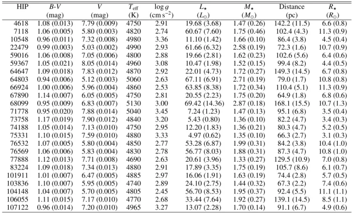
parallax (see Table2), the total luminosity of the giant is fixed. This allows accurately determining the amount of missing light from the SED fit. For two systems, HIP 4618 (see Fig. 1) and HIP 59367, the SED fit shows that about 4–5% of the total light originates from the companion. For all other systems the contribution of the com-panion to the total light is lower than 1%. This contribution is too low for spectral separation to work or to determine in any way reliable parameters for the companion star.

None of the model SEDs based on the spectroscopically ob-tained parameters shows a surplus luminosity compared to liter-ature photometry. This is an additional indication of the correct-ness of the giant companion’s spectroscopic parameters.

4000 10000 20000

Wavelength ˚A 0

5 10 15 20

Fλ

·

10

8(erg/s/c

m

2)

U B1

B B2

V1 V G

J

H

Ks

Fig. 1.Example SED fit for HIP 4618. The best-fitting binary model is shown with black dots, with the integrated model photometry in black crosses. The observed photometry is shown in red, with the horizon-tal error bar the width of the pass band. The parameters for this fit are for the giantTeff =4750 (100) K, logg =2.91, radius=6.6 (0.8)R (see Table 2), and for the companion Teff = 5500 K, logg = 4.0,

radius=1.2R.

4. Orbital elements

(4)

Table 3.Orbital elements of the binary companions.

HIP 4618* HIP 10548* HIP 59367 HIP 83224* HIP 73758* HIP 104148 P(days) 211.4 (0.03) 429.1 (0.25) 2779.3 (84.29) 173.3 (0.03) 97.1 (0.002) 1599.3 (8.15) T0(JD-2 450 000) 5406.3 (0.32) 5306.6 (1.51) 4832.7 (13.07) 5251.3 (0.1) 5304.3 (0.03) 3878.5 (3.59)

e 0.1 (0.003) 0.3 (0.003) 0.8 (0.13) 0.3 (0.001) 0.4 (0.0006) 0.2 (0.00)

ω(deg) 40.8 (0.58 ) 5.0 (1.86) 235.7 (15.68) 85.6 (0.29) 53.4 (0.08) 194.4 (2.40) K(m s−1₎ _{12 939.2 (7.84 )} _{6942.8 (29.82)} _{5947.6 (182.71)} _{8742.5 (6.91)} _{11 817.4 (11.00)} _{5581.3 (5.42)}

f(M) (10−3M) 46.7 (0.09) 12.9 (0.17) 13.1 (6.9) 10.4 (0.03) 12.8 (0.04) 27.1 (0.16)

Notes.The systems with (*) a have a full orbital coverage. Mass function f(M)=m2 2sin

3_i_/(_m 1+m2)2.

HIP4618 HIP10548

HIP59367 HIP73758

HIP83224 HIP104148

Fig. 2.RV variations of the six binary systems with reliable orbital so-lution. The black circles, blue squares, green crosses, and red triangles correspond to FEROS, CHIRON, UCLES, and PUCHEROS data, re-spectively. The best orbital solutions are overplotted (solid line). The post-fit RMS is typically∼10 m s−1_.

time span is longer than the orbital period and for wich thus a reliable orbital solution can be derived; (ii) systems with longer orbital periods, for which it is possible to obtain a solution, but with a high level of degeneracy in the orbital parameters; and (iii) systems that present a RV trend.

4.1. Short-period binaries

Four of the 24 stars, show large RV variations (&10 km s−1_{), with}

orbital periodsP.430 days. For these, it was possible to fully constrain the orbital solution. To determine the orbital elements of the systems, we used the 2.17 version of the Systemic Console (Meschiari et al. 2009), excluding the PUCHEROS velocities, which have uncertainties up to∼100 times larger than UCLES, FEROS, and CHIRON data. The stars HIP 4618, HIP 10548, HIP 73758, and HIP 83224 have periods shorter than∼430 days. The orbital elements of the four stellar companions are listed in Table 3. Figure 2 shows the resulting RV curves. In the four cases, the RV data cover more than two orbital periods.

4.2. Long-period binaries

In eight cases, we observe large RV variations, but with orbital periods exceeding the observational time span. However, for HIP 59367 and HIP 104148 the phase coverage is good enough to obtain a unique orbital solution. Figure2shows the RV curves of these two stars. The orbital elements of the binary companions are listed in Table3.

HIP59016 HIP67890

HIP64803 HIP66924

HIP76532 HIP76569

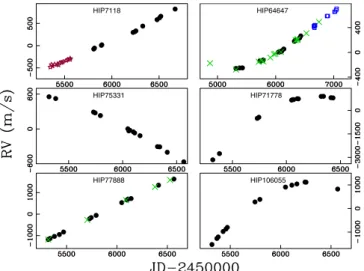
Fig. 3.RV variations of six long-period binaries. The black circles, blue squares, green crosses, brown open stars, and red triangles correspond to FEROS, CHIRON, UCLES, FECH, and PUCHEROS data, respectively. In each case, one possible orbital solution is overplotted (solid line).

For the remaining six cases the orbital solution is partially degenerated because of the poor phase coverage, meaning that we can only set lower and upper limits for the orbital period and the eccentricity. Figure3shows the RV curve of these stars. One possible orbital solution is overplotted. In these cases it is not possible to unambiguously obtain a solution.

4.2.1. Long-period trends

The remaining 12 stars in this sample present RV variations, ranging from thousands of m s−1level up to peak-to-peak varia-tions of several km s−1_{. Half of the systems present a linear RV}

trend, while the remainder show some level of curvature in the observed velocities. Figure 4 shows the RV epochs of the six stars that present the smallest RV variations (∼500 m s−1_{). Since}

these stars show moderate RV variations, they are candidates for hosting long-period brown dwarfs, which makes them very in-teresting targets for direct imaging to determine the nature of the companion. Finally, Fig.5shows the velocity variations of the stars that present large RV long-trend variations (&1 km s−1_),

which are most likely part of a long-period stellar binary system.

5. Metallicity distribution

(5)

HIP22479 HIP68099

HIP74188 HIP101911

HIP103836 HIP107122

Fig. 4.RV variations of six long-period brown dwarf companion can-didates. The black filled circles, blue squares, green crosses, brown open stars, and magenta open circles correspond to FEROS, CHIRON, UCLES, FECH, and HARPS data, respectively.

HIP7118 HIP64647

HIP75331 HIP71778

HIP77888 HIP106055

Fig. 5. Long-period RV trends of six binary systems. The black cir-cles, blue squares, brown open stars, and green crosses correspond to FEROS, CHIRON, FECH, and UCLES data, respectively.

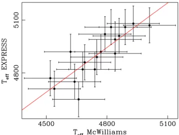
We computed the metallicities of SET04 targets using FEROS archival data. For the MAS08 targets, we used only those targets with metallicities computed by McWilliam (1990, MCW90 hereafter). We compared our sample with the MCW90 sample and we found 18 common stars. These stars are shown in Fig.6. To remove any bias due to differences in the metallicity derived by our method and MCW90, we adjusted a linear func-tion to correlate the two studies. We found a linear correlafunc-tion of the form [Fe/H]EXP=1.20 [Fe/H]MCW90+0.17. Figure6shows

the EXPRESS versus MCW90 metallicities for the 18 targets in common. The best linear fit is overplotted. The RMS of the fit is 0.08 dex, and the Pearson linear coefficient isr=0.90.

Using this information, we converted from MCW90 metal-licities into our metallicity scale, for all of the binaries listed in MAS08 and metallicities from MCW90. Figure7shows the nor-malized metallicity distribution of the primary stars for a total of 59 binaries, including EXPRESS, SET04, and MAS08 systems (black solid line). The error bars were computed according to Cameron (2011). The overall sample distribution is overplotted (blue dashed line). The metallicity distribution between∼−0.3 to 0.3 dex is nearly flat. Moreover, the highest fraction is obtained

Fig. 6. EXPRESS versus MCW90 metallicities for the 18 targets in common. The red line corresponds to the belinear fit.

Fig. 7.Normalized histogram of the metallicity distribution of the pri-mary stars (black solid line). The overall metallicity distribution of the parent sample is overplotted (dashed blue line). The width of the bins is 0.2 dex.

at metallicities around−0.5 dex. Interestingly, Raghavan et al. (2010) showed that binary systems among solar-type stars red-der than B−V = 0.625 are more frequent around stars with [Fe/H].−0.3 dex, in good agreement with our findings1. How-ever, we note that the bin centered on−0.5 dex in the one with the least number of stars in the combined sample (13 systems), and therefore with the largest error bars. This result is in stark con-trast with the observed metallicity distribution of planet-hosting giant stars, showing a strong increase in the giant planet fre-quency with increasing metallicity (e.g., Reffert et al. 2015; Jones et al.2016), as found in solar-type stars (e.g., Fischer & Valenti2005). This observational result also agrees with recent hydrodynamical simulations showing that the formation of bi-nary systems across a wide range of stellar masses is not sig-nificantly affected by the metal content of the molecular clouds (Bate2014).

Additionally, we also studied the relation in the effective temperatures (Teff) for these 18 stars in common. We compared

the McWilliam and ourTeff values and found a linear

correla-tion of the formTeff(EXP)=0.84Teff (MCW90)+889.1. The

(6)

Fig. 8.EXPRESS versus MCW90 effective temperatures (Teff) for the

18 targets in common. The red line corresponds to the best linear fit.

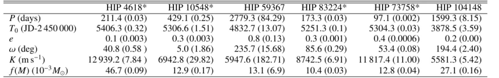
Fig. 9.Orbital period versus eccentricity for 130 spectroscopic giant binary stars. The red open circles represent our binaries with well-constrained orbital periods, while the blue filled circles represent those with poorly constrained orbits. The black dots, magenta filled triangles, and green filled squares correspond to MAS08, VER95, and SET04 bi-naries, respectively.

Pearson linear coefficient is r = 0.84. Figure 8 shows the MVW90 versus EXPRESS Teffs. The linear fit is overplotted.

The error bars are not given in the MC90, and we used error bars given by the standard deviation for deTeff (MC90) values. Our

values overestimate those derived by MCW90, which mainly ex-plains why we also see a systematic difference in the derived metallicities (see Fig.6).

6. Period-eccentricity distribution

We studied the period-eccentricity distribution of 130 spectro-scopic binary systems in giant stars. We included all of the bi-naries with orbital solution from VER95, SET04, MAS08, and those presented here for which it was possible to obtain an orbital solution. Figure 9 shows the orbital period versus ec-centricity of these systems. Systems with short orbital periods (P.20 days) present nearly circular orbits, similar to solar-type binaries, which is most likely explained by tidal circularization. Furthermore, there is a transition region from P ∼20–80 days

where binary systems present moderate eccentricities (e.0.4). Finally, at longer orbital periods, there is a wide spread in e, ranging from nearly circular orbits to highly eccentric systems (e∼0.9). This transition region and eccentricity distribution at orbital periods longer than∼100 d is also observed in solar-type binaries (e.g., Duquennoy & Mayor1991; Jenkins et al.2015).

The giant binary systems with moderately long orbital peri-ods (∼400–800 days) might be the precursors of the wide ec-centric hot subdwarf binaries studied by Vos et al. (2015). A hot subdwarf star is a core helium-burning star located at the blue end of the horizontal branch, with colours similar to main-sequence B stars, but with much broader Balmer lines (Sargent & Searle 1968). The study of the orbital parameters of these systems will therefore be useful in binary population synthesis studies for wide sdB binaries to help determine the correct evo-lutionary channels of these evolved binaries.

7. Summary

We presented a sample of 24 giant stars that have revealed large radial velocity variations, which are induced by massive sub-stellar or sub-stellar companions. Based on precision RVs computed from high-resolution spectroscopic observations obtained as part of the EXPRESS program, we were able to fully constrain the orbital elements of 6 systems. In 6 more cases, we were able to obtain a solution although the orbital elements are poorly con-strained. In the remaining cases, the primary star exhibits a RV trend, thus no solution is obtained. Six of these stars present ve-locity variations that are compatible with the presence of a long-period brown dwarf companion.

In addition, we studied the metallicity distribution of the pri-mary stars. For this purpose, we retrieved literature data from two different studies, namely MAS08 and SET04. Our final sam-ple comprised 59 spectroscopic binary systems, detected from a parent sample of 395 giant stars, covering a range of metallici-ties between [Fe/H]∼ −0.5 and+0.5 dex. We found no signif-icant correlation between the frequency of binary companions and the stellar metallicity. This result reinforces the fact that stel-lar binaries are formed mainly by gravitational collapse, which is highly insensitive to the dust content of the protostellar disk (e.g., Bate2014), while planetary systems, including those or-biting giant stars, are formed in the protoplanetary disk by the core-accretion mechanism (e.g., Gonzalez,1997; Santos et al. 2001; Reffert et al.2015; Jones et al.2016).

Finally, we studied the period-eccentricity distribution of the companions. We included a total of 130 spectroscopic binaries from the literature with known eccentricities. We found an ec-centricity distribution that is characterized by short-period sys-tems (P . 20 days) that present very low eccentricities (with the exception of one case withe∼0.2). For orbital periods be-tween∼20–80 days, all of the systems present moderate orbital eccentricities (e.0.4). At longer orbital periods, there is a wide spread ine, from nearly circular orbits to eccentricities as high as ∼0.9. The overall distribution is qualitatively similar to the distribution observed in solar-type stars, although the circular-ization edge is found at slightly longer orbital periods, which is most likely explained by the stronger tidal effect induced by the larger stellar radii.

(7)

(CATA) PFB–06/2007. F.O.E. acknowledges support from FONDECYT through postdoctoral grant 3140326 and from project IC120009 “Millennium Institute of Astrophysics (MAS)” of the Iniciativa Científica Milenio del Ministerio de Economía, Fomento y Turismo de Chile.

References

Alonso, A., Arribas, S., Benz, W., & Martínez-Roger, C. 1999,A&A, 140, 261 Arenou, F., Grenon, M., & Gómez, A. 1992,A&A, 258, 104

Baranne, A., Queloz, D., Mayor, M., et al. 1996,A&A, 119, 373 Bate, M. R. 2014,MNRAS, 442, 285

Butler, R. P., Marcy, G. W., Williams, E., et al. 1996,PASP, 108, 500 Cameron, E. 2011,PASA, 28, 128

Degroote, P., Acke, B., Samadi, R., et al., 2011,A&A, 536, A82

Diego, F., Charalambous, A., Fish, A. C., & Walker, D. D. 1990, Proc. Soc.Photo-Opt. Instr. Eng., 1235, 562

Duquennoy, A., & Mayor, M. 1991,A&A, 248, 485 Endl, M., Kurster, M., & Els, S. 2000,A&A, 362, 585 Fischer, D. A., & Valenti, J. 2005,ApJ, 622, 1102 Gonzalez, G. 1997,MNRAS, 285, 403

Jenkins, J. S., Díaz, M., Jones, H. R. A., et al. 2015,MNRAS, 453, 1439 Jones, M. I., Jenkins, J. S., Rojo, P., & Melo, C. H. F. 2011,A&A, 536, A71 Jones M. I., Jenkins J. S., Rojo P., Melo C. H. F., Bluhm P., 2013,A&A, 556,

A78

Jones, M. I., Jenkins, J. S., Rojo, P., et al. 2015,A&A, 580, A14 Jones, M.I., Jenkins, J.S, Brahm, R., et al. 2016A&A, 590, A38 Kaufer, A., Stahl, O., Tubbesing, S., et al. 1999,The Messenger 95, 8 Kurucz, R.L., 1979ApJ, 40, 1

Kurucz, R. L., 1993, ATLAS9 Stellar Atmosphere Programs and 2 km s−1_Grid,

CD-ROM No. 13 (Cambridge, Smithsonian Astrophysical Observatory)

Lada, C. J. 2006,ApJ, 640, L63 Machida M. N. 2008,ApJ, 682, 1

Massarotti, A., Latham, D., Stefanik, R. P., & Fogel, J. 2008,AJ, 135, 209 Mayor, M., Pepe, F., Queloz, D., et al. 2003,The Messenger, 114, 20 McWilliam, A. 1990,ApJS, 74, 1075

Meschiari, S., Wolf, A. S., Rivera, E., et al. 2009,PASJ, 121, 1016 Pan, K., Tan, H., Duan, C., & Shan, H. 1998ASP Conf., 138, 267

Perryman, M. A. C., Lindegren, L., Kovalevsky, J., et al. 1997,A&A, 343, L49 Raghavan, D., McAlister, H. A., Henry, T. J., et al. 2010,ApJ, 190, 1 Reffert, S., Bergmann, C., Quirrenbach, A., et al. 2015,A&A, 574, A116 Salasnich, L., Girardi, L., Weiss, A., & Chiosi, C. 2000,A&A, 361, 1023 Santos, N. C., Israelian, G., & Mayor, M. 2001,A&A, 373, 1019 Sargent, W. L. W., & Searle, L. 1968,ApJ, 152, 443

Sato, B., Izumiura, H., Toyota, E., et al. 2008,PASJ, 60, 539 Setiawan, J., Pasquini, L., & da Silva, L. 2004,A&A, 421, 241 Sneden, C. 1973,ApJ, 184, 839

Tassoul, J. L. 1987,ApJ, 322, 856 Tassoul, J. L. 1988,ApJ, 324, 71 Tassoul, J. L. 1992,ApJ, 395, 259

Tokovinin, A., Fisher, D., Bonati, M. et al. 2013,PASP, 125, 1336 Tonry, J., & Davis, M., 1979,AJ, 84, 1511

Vanzi, L., Chacon, J., Helminiak, K.G., et al. 2012,MNRAS, 424, 2770 Verbunt, F., & Phinney, E. S. 1995,A&A, 296, 709

Villaver, E., & Livio, M. 2009,ApJ, 705, 81

Vos, J., Østensen, R. H., Degroote, P., et al. 2012,A&A, 548, A6 Vos, J., Østensen, R. H., Németh, P., et al. 2013,A&A, 559, A54 Vos, J., Østensen, R. H., Marchant, P., et al. 2015 A&A, 579, A49 Wittenmyer, R. A., Endl, M., Wang, L., et al. 2011,ApJ, 743, 184 Wittenmyer, R. A., Butler, R. P., Wang, L., et al. 2016,MRAS, 455, 138 Zahn, J. P. 1977,A&A, 57, 383

(8)

Appendix A: Radial velocity tables

Table A.1.Radial velocity variations for HIP 4618.

JD RV err Instrument

−2 450 000 (ms−1₎ _(ms−1₎

5140.11 −3.4 1.8 UCLES

5525.95 −11 966.3 2.7 UCLES

5601.93 7339.9 3.3 UCLES

5457.74 −7583.3 5.2 FEROS

5470.78 −9871.8 7.3 FEROS

6056.93 5693.4 5.5 FEROS

6099.92 −9187.2 6.3 FEROS

6160.95 −3752.3 7.7 FEROS

6230.65 15 340.8 5.0 FEROS

6231.79 15 371.9 4.5 FEROS

6331.53 −10 427.0 7.7 FEROS

6431.93 14 269.6 6.3 FEROS

6472.95 8653.4 5.5 FEROS

6537.92 −10 493.3 4.3 FEROS

6565.72 −8014.1 5.4 FEROS

6561.57 −6387.6 121.2 PUCHEROS 6569.73 −4962.8 106.7 PUCHEROS 6582.71 −1780.8 76.0 PUCHEROS 6608.63 6535.8 90.2 PUCHEROS 6638.57 15 857.5 131.8 PUCHEROS 6643.63 16 447.2 199.5 PUCHEROS 6650.58 17 404.8 144.9 PUCHEROS 6653.59 17 881.8 136.9 PUCHEROS 6660.56 17 340.9 115.1 PUCHEROS 6664.58 16 870.5 145.9 PUCHEROS 6668.61 15 979.9 124.2 PUCHEROS 6678.55 13 211.7 110.6 PUCHEROS

−2 450 000 (ms−1₎ _(ms−1₎

5347.90 −484.3 14.3 FECH 5359.89 −428.9 14.4 FECH 5373.86 −460.1 13.0 FECH 5393.85 −422.5 16.5 FECH 5421.75 −422.7 13.5 FECH 5435.71 −436.0 14.0 FECH 5449.67 −385.1 15.8 FECH 5467.64 −382.8 12.6 FECH 5482.64 −366.9 21.4 FECH 5517.62 −336.0 13.3 FECH 5531.62 −316.0 13.3 FECH 5557.61 −314.3 14.3 FECH 5558.62 −287.6 15.0 FECH 5807.93 −76.4 7.7 CHIRON 5815.88 −55.1 10.6 CHIRON

5888.74 7.3 8.0 CHIRON

5893.62 19.3 7.9 CHIRON

6224.60 299.0 8.1 CHIRON

6244.61 316.6 6.8 CHIRON

6253.64 332.5 7.5 CHIRON

6326.56 441.4 7.2 CHIRON

6477.89 585.3 6.9 CHIRON

6505.91 631.1 7.2 CHIRON

6517.85 663.2 8.0 CHIRON

6669.57 825.6 6.8 CHIRON

6870.80 1053.2 7.0 CHIRON

Table A.3.Radial velocity 10548.

−2 450 000 (ms−1) (ms−1)

5457.79 −5857.7 5.2 FEROS 5470.81 −6206.9 6.3 FEROS 5729.92 7223.3 10.4 FEROS

6160.86 7205.0 2.5 FEROS

6230.71 262.4 5.5 FEROS

6241.73 −963.4 5.3 FEROS 6251.75 −1975.6 4.7 FEROS 6321.57 −6032.3 7.1 FEROS 6331.58 −6282.4 7.4 FEROS

6565.75 5874.6 5.7 FEROS

(9)

−2 450 000 (ms−1₎ _(ms−1₎

4085.64 107.4 0.2 HARPS

4371.79 76.7 0.3 HARPS

4561.49 64.6 0.2 HARPS

4684.91 36.3 0.3 HARPS

4787.76 26.4 0.3 HARPS

4788.79 25.6 0.2 HARPS

4858.55 29.5 0.3 HARPS

4891.58 28.4 0.3 HARPS

4893.59 33.2 0.4 HARPS

5075.87 102.1 12.3 FECH

5084.91 97.8 11.9 FECH

5093.92 94.2 11.7 FECH

5104.82 122.8 12.5 FECH

5166.71 112.6 10.8 FECH

5421.89 69.2 12.6 FECH

5435.87 82.4 11.7 FECH

5449.89 83.6 11.9 FECH

5467.79 79.3 11.2 FECH

5482.74 73.2 14.4 FECH

6011.55 9.5 9.2 CHIRON

6019.52 −13.0 6.7 CHIRON

6226.82 −7.0 6.3 CHIRON

6239.72 −0.7 5.6 CHIRON

6248.69 1.3 4.8 CHIRON

6539.88 −29.0 9.7 CHIRON 6547.89 −42.8 6.3 CHIRON 6557.82 −23.9 6.3 CHIRON 6563.72 −48.9 6.1 CHIRON 6690.58 −51.0 5.0 CHIRON 6711.54 −54.3 5.6 CHIRON 6720.62 −67.6 8.8 CHIRON 6723.50 −72.8 5.6 CHIRON 6734.49 −38.9 5.6 CHIRON 6745.48 −62.8 5.7 CHIRON 6888.92 −54.2 6.1 CHIRON 6976.79 −86.2 5.2 CHIRON 6976.79 −86.4 5.4 CHIRON 7019.69 −92.4 5.8 CHIRON 7027.66 −96.3 5.6 CHIRON

−2 450 000 (ms−1₎ _(ms−1₎

3072.75 −723.8 6.6 FEROS 5317.51 −707.8 5.1 FEROS 5379.50 −617.9 3.1 FEROS 5428.48 −562.7 5.1 FEROS 5729.54 −255.8 10.2 FEROS 5744.49 −244.5 5.6 FEROS 5786.48 −216.4 4.5 FEROS

6047.52 11.4 5.6 FEROS

6056.51 1.3 5.5 FEROS

6099.50 69.3 4.8 FEROS

6110.48 56.6 4.0 FEROS

6140.52 80.1 4.6 FEROS

6160.47 98.5 4.2 FEROS

6321.69 262.7 7.6 FEROS

6331.68 247.6 7.8 FEROS

6342.64 288.5 7.8 FEROS

6412.53 322.3 4.3 FEROS

6412.73 323.2 4.7 FEROS

6431.57 355.8 5.7 FEROS

6472.54 394.8 4.9 FEROS

7072.78 816.7 8.7 FEROS

4866.23 −1166.6 2.5 UCLES 5380.88 −563.1 2.4 UCLES 5580.23 −367.3 2.8 UCLES 5706.91 −244.9 4.8 UCLES

5970.19 0.0 2.9 UCLES

6090.97 119.4 4.3 UCLES

6345.14 339.6 2.9 UCLES

6376.09 374.8 2.6 UCLES

(10)

−2 450 000 (ms−1₎ _(ms−1₎

4866.22 −112.0 2.5 UCLES

5581.19 1436.2 2.4 UCLES

5970.19 698.5 2.8 UCLES

6059.98 542.1 4.8 UCLES

6088.92 486.8 2.9 UCLES

6344.14 0.0 4.3 UCLES

6376.04 −62.6 2.9 UCLES

6378.01 −66.8 2.6 UCLES

6748.08 −897.2 2.3 UCLES

5317.53 1755.5 5.1 FEROS

5379.51 1608.1 3.8 FEROS

5729.54 879.4 6.0 FEROS

5744.50 860.4 5.9 FEROS

6047.52 296.8 3.8 FEROS

6056.52 275.2 3.9 FEROS

6066.53 252.2 5.0 FEROS

6099.52 200.2 5.0 FEROS

6110.48 168.0 4.7 FEROS

6140.53 101.7 6.9 FEROS

−2 450 000 (ms−1₎ _(ms−1₎

4870.21 −151.9 2.8 UCLES 5317.98 −254.3 1.6 UCLES 5706.96 −129.2 2.2 UCLES 5757.89 −110.0 5.9 UCLES 5787.87 −123.0 3.5 UCLES

5908.24 −60.6 2.2 UCLES

5969.23 −6.6 2.0 UCLES

5995.19 0.0 2.1 UCLES

6088.95 29.0 2.6 UCLES

6344.19 218.1 3.3 UCLES

6345.12 220.1 3.1 UCLES

6376.11 223.4 2.4 UCLES

6377.06 237.5 3.1 UCLES

6528.85 331.9 3.7 UCLES

6745.09 515.9 2.3 UCLES

5317.57 −261.1 6.6 FEROS 5379.67 −252.3 4.9 FEROS 5428.49 −251.4 6.6 FEROS 5729.59 −137.8 12.3 FEROS 5744.55 −142.7 6.7 FEROS 5786.55 −123.4 5.3 FEROS

6047.58 2.7 7.7 FEROS

6056.56 1.7 5.7 FEROS

6066.58 11.5 6.9 FEROS

6099.56 11.5 7.1 FEROS

6110.54 28.2 6.5 FEROS

6140.58 54.0 4.6 FEROS

6321.75 179.2 7.0 FEROS

6331.77 184.4 7.5 FEROS

6342.72 198.7 7.9 FEROS

6412.70 231.5 4.6 FEROS

6431.62 265.3 6.8 FEROS

6655.79 −119.5 5.8 CHIRON 6660.81 −121.9 6.5 CHIRON 6664.79 −107.1 6.1 CHIRON 6668.85 −141.1 6.5 CHIRON 6672.88 −98.8 6.1 CHIRON 6678.80 −103.5 5.6 CHIRON

6883.51 47.0 6.2 CHIRON

6894.48 47.8 6.3 CHIRON

6898.47 50.6 6.0 CHIRON

7013.85 116.6 5.3 CHIRON

7021.85 119.8 5.1 CHIRON

7039.84 143.3 4.8 CHIRON

(11)

−2 450 000 (ms−1₎ _(ms−1₎

3072.81 −226.8 25.0 FEROS

5317.57 −1296.4 5.0 FEROS

5379.64 −1183.7 4.3 FEROS

5729.60 −484.8 12.7 FEROS

5729.60 −485.7 11.6 FEROS

5729.61 −491.9 12.5 FEROS

5744.55 −449.3 5.5 FEROS

5744.55 −466.6 5.6 FEROS

6047.58 −60.6 6.7 FEROS

6047.58 −56.0 6.3 FEROS

6047.58 −62.2 7.2 FEROS

6056.57 −39.2 5.1 FEROS

6056.57 −38.1 4.6 FEROS

6066.58 −28.1 5.3 FEROS

6066.58 −33.2 5.1 FEROS

6099.56 −10.5 5.5 FEROS

6110.54 −8.8 4.5 FEROS

6140.58 35.3 4.8 FEROS

6533.47 −106.2 4.9 CHIRON

6644.85 −65.8 11.9 CHIRON

6645.85 −68.7 5.2 CHIRON

6648.85 −62.7 9.7 CHIRON

6655.81 −64.5 4.3 CHIRON

6666.84 −57.2 4.3 CHIRON

6673.85 −57.0 4.3 CHIRON

6707.84 −40.5 4.5 CHIRON

6721.75 −28.7 4.3 CHIRON

6735.61 −24.7 4.4 CHIRON

6751.76 −20.6 4.9 CHIRON

6769.53 −23.1 4.8 CHIRON

6784.61 −16.8 4.6 CHIRON

6827.52 −2.1 4.2 CHIRON

6876.46 19.8 9.3 CHIRON

Table A.9.Continued table for HIP 64803.

−2 450 000 (ms−1₎ _(ms−1₎

3072.83 −1277.9 20.0 FEROS

5317.623 312.2 5.1 FEROS

6321.79 −395.5 7.4 FEROS

6321.79 −392.5 6.9 FEROS

6342.75 −421.7 7.1 FEROS

6342.75 −427.4 7.5 FEROS

6412.61 −655.7 3.7 FEROS

6431.65 −708.8 6.4 FEROS

6391.60 −712.5 80.9 PUCHEROS 6398.58 −477.5 61.6 PUCHEROS 6400.56 −562.8 65.3 PUCHEROS 6407.59 −463.1 70.9 PUCHEROS 6413.62 −583.7 69.5 PUCHEROS 6421.61 −611.8 63.3 PUCHEROS 6682.81 −1879.2 73.0 PUCHEROS 6695.75 −1550.4 63.8 PUCHEROS 6709.74 −1658.5 67.8 PUCHEROS 6745.68 −1808.4 61.8 PUCHEROS 6770.62 −1745.6 64.5 PUCHEROS 6785.56 −1894.7 61.4 PUCHEROS

6888.49 230.3 3.7 CHIRON

6904.47 178.8 3.8 CHIRON

6922.48 132.2 4.5 CHIRON

(12)

−2 450 000 (ms−1₎ _(ms−1₎

3071.68 2347.3 40.0 FEROS

5317.64 369.7 5.1 FEROS

5379.65 284.3 4.4 FEROS

5428.53 254.4 5.1 FEROS

5729.64 −39.0 11.1 FEROS 5729.64 −43.1 10.2 FEROS

5744.61 −53.9 5.3 FEROS

5744.61 −57.8 5.0 FEROS

6047.63 −210.4 5.7 FEROS 6047.63 −216.4 6.4 FEROS 6056.61 −235.1 4.9 FEROS 6066.63 −239.6 5.1 FEROS 6099.61 −227.2 4.4 FEROS 6110.59 −247.0 4.3 FEROS 6140.59 −238.6 4.0 FEROS 6140.60 −241.7 3.8 FEROS 6321.80 −223.1 6.8 FEROS 6321.80 −222.5 6.9 FEROS 6342.79 −202.6 7.6 FEROS 6342.79 −197.0 7.0 FEROS 6412.71 −178.3 3.2 FEROS 6431.65 −182.5 5.4 FEROS

4868.25 874.1 1.3 UCLES

5227.21 439.0 1.4 UCLES

5380.95 241.6 1.6 UCLES

5580.26 15.9 1.4 UCLES

5602.18 2.9 1.9 UCLES

6060.06 −251.5 2.5 UCLES 6090.96 −252.4 1.8 UCLES 6345.15 −255.6 1.5 UCLES 6376.21 −233.1 1.7 UCLES 6527.87 −147.8 3.7 UCLES

−2 450 000 (ms−1₎ _(ms−1₎

5317.64 −187.5 5.1 FEROS 5379.66 −162.6 4.5 FEROS 5729.65 −34.1 11.7 FEROS

5744.62 −63.4 6.2 FEROS

6047.64 −6.4 6.1 FEROS

6056.64 −24.1 4.8 FEROS

6066.64 −11.4 5.7 FEROS

6099.62 19.8 5.8 FEROS

6110.59 4.1 5.2 FEROS

6140.60 25.1 4.0 FEROS

6321.81 72.9 6.9 FEROS

6342.78 86.4 7.1 FEROS

6412.72 98.0 3.8 FEROS

6412.75 92.5 4.4 FEROS

6431.66 90.7 6.6 FEROS

6531.49 −47.9 6.1 CHIRON 6654.84 −58.0 4.6 CHIRON 6656.83 −53.6 4.7 CHIRON

6673.87 1.7 7.0 CHIRON

6679.83 22.1 7.0 CHIRON

6695.88 −13.9 5.3 CHIRON 6708.82 −12.6 6.7 CHIRON

6722.70 −9.7 5.5 CHIRON

6736.64 −10.7 5.4 CHIRON 6752.69 −29.0 5.1 CHIRON 6769.66 −31.0 4.5 CHIRON 6790.54 −28.0 5.4 CHIRON

6810.60 9.5 5.1 CHIRON

6833.58 28.8 4.9 CHIRON

6887.47 −19.6 7.3 CHIRON

6908.47 2.5 4.5 CHIRON

7018.85 29.8 5.4 CHIRON

7025.85 25.4 4.4 CHIRON

7034.82 14.8 4.7 CHIRON

7050.79 48.0 4.7 CHIRON

7050.80 45.6 5.3 CHIRON

7061.78 46.6 5.0 CHIRON

7063.83 39.0 5.3 CHIRON

−2 450 000 (ms−1₎ _(ms−1₎

5317.69 −3148.7 7.9 FEROS 5379.67 −2756.6 6.9 FEROS 5729.68 −512.2 12.5 FEROS 5744.65 −439.9 7.4 FEROS

6047.63 649.3 8.1 FEROS

6056.67 677.7 6.0 FEROS

6066.67 685.1 5.5 FEROS

6099.66 741.4 6.9 FEROS

6110.62 732.4 5.9 FEROS

6321.85 886.4 8.8 FEROS

6342.87 891.5 8.9 FEROS

6412.77 803.7 5.9 FEROS

(13)

−2 450 000 (ms−1₎ _(ms−1₎

4871.25 0.0 2.4 UCLES

5318.06 −4836.2 1.2 UCLES

5971.20 14359.2 1.6 UCLES

6378.18 2138.4 2.0 UCLES

5317.71 −6956.8 5.1 FEROS

5729.70 −6061.2 10.3 FEROS

5744.67 −2403.2 5.8 FEROS

5793.61 3287.7 5.1 FEROS

6047.69 1412.5 6.9 FEROS

6056.69 5293.0 5.0 FEROS

6066.69 11047.3 5.3 FEROS

6099.68 −8026.5 5.2 FEROS

6110.66 −7397.2 4.3 FEROS

6160.59 9045.7 3.2 FEROS

6321.86 −3898.7 7.6 FEROS

6342.89 2985.1 7.2 FEROS

6412.63 −5389.0 3.5 FEROS

6412.76 −5368.4 3.9 FEROS

6431.72 −119.0 6.1 FEROS

6565.49 12548.5 5.2 FEROS

6047.69 −36.1 8.3 FEROS

6056.69 −65.6 4.1 FEROS

6066.69 −60.2 4.8 FEROS

6099.68 −71.1 4.7 FEROS

6110.64 −81.1 4.4 FEROS

6140.65 −85.4 4.3 FEROS

6321.87 −182.3 7.8 FEROS 6342.89 −193.4 7.6 FEROS 6412.79 −219.9 4.5 FEROS

6056.72 −33.7 5.0 FEROS

6066.72 −24.1 5.8 FEROS

6099.71 −51.3 4.4 FEROS

6110.67 −68.8 4.7 FEROS

6160.58 −116.7 4.0 FEROS 6321.89 −305.5 6.8 FEROS 6342.92 −308.9 7.2 FEROS 6412.83 −402.4 3.6 FEROS 6565.48 −567.3 6.4 FEROS

−2 450 000 (ms−1) (ms−1)

3070.79 −4730.0 20.0 FEROS

5317.75 2842.4 5.1 FEROS

5334.85 1932.0 15.7 FECH

(14)

−2 450 000 (ms−1₎ _(ms−1₎

3070.77 −1487.9 20.0 FEROS

5470.48 3769.7 9.0 FEROS

5729.76 2758.5 10.1 FEROS 5729.76 2748.3 11.9 FEROS

5744.71 2700.9 7.0 FEROS

5744.71 2695.1 6.6 FEROS

6047.72 381.2 6.2 FEROS

6047.72 381.5 6.9 FEROS

6066.72 254.4 6.3 FEROS

6066.72 257.1 6.5 FEROS

6099.71 35.8 6.3 FEROS

6140.66 −323.6 4.5 FEROS 6140.66 −317.9 4.6 FEROS 6160.60 −434.4 4.9 FEROS 6160.61 −435.8 5.1 FEROS 6412.80 −1835.2 4.2 FEROS 6431.73 −1895.6 7.1 FEROS 6565.49 −2462.6 5.4 FEROS 7072.89 −3392.8 7.9 FEROS 7072.89 −3397.0 7.3 FEROS

5317.85 2058.7 13.9 FECH

5326.85 2097.8 17.7 FECH

5334.86 2058.5 17.1 FECH

5359.78 2082.6 13.8 FECH

5373.63 2111.7 14.2 FECH

5390.66 2132.8 13.9 FECH

5421.58 2063.5 21.1 FECH

5435.58 2059.1 18.2 FECH

5701.85 1187.7 15.8 CHIRON 5704.85 1186.3 13.4 CHIRON 5725.77 981.8 14.6 CHIRON 5742.71 938.1 13.8 CHIRON 5767.49 763.6 11.9 CHIRON

5782.62 733.6 9.9 CHIRON

5804.57 544.9 9.8 CHIRON

6040.69 −1294.1 7.1 CHIRON 6050.69 −1383.5 7.2 CHIRON 6892.48 −4973.9 7.8 CHIRON 6918.48 −5012.0 6.7 CHIRON 7060.85 −5155.3 6.8 CHIRON 7091.78 −5182.0 6.5 CHIRON

−2 450 000 (ms−1₎ _(ms−1₎

5793.63 −59.2 4.2 FEROS

6047.73 532.2 7.2 FEROS

6099.73 654.9 6.0 FEROS

6110.69 695.9 5.7 FEROS

6140.67 721.1 4.3 FEROS

6412.66 1341.6 4.8 FEROS

6565.51 1626.8 6.8 FEROS

5319.11 −1828.3 1.4 UCLES 5707.09 −919.3 2.3 UCLES

6090.13 0.0 2.9 UCLES

6377.16 614.7 2.7 UCLES

6526.95 938.3 4.3 UCLES

(15)

−2 450 000 (ms−1₎ _(ms−1₎

5319.17 −0.2 0.6 UCLES

5382.06 10851.2 0.9 UCLES

5379.77 7098.4 5.0 FEROS

5428.63 −1423.7 4.5 FEROS

5457.56 −8124.6 4.6 FEROS

5470.54 −6797.2 9.5 FEROS

5744.75 9187.8 4.8 FEROS

5786.64 −6707.6 4.9 FEROS

5793.65 −8008.5 5.8 FEROS

6047.76 2769.6 7.7 FEROS

6066.75 6081.5 6.4 FEROS

6160.63 −7192.9 4.1 FEROS

6412.84 5981.0 5.4 FEROS

6431.75 8740.5 7.3 FEROS

6472.76 −3940.8 5.5 FEROS

6565.52 2336.6 4.8 FEROS

6561.49 −17661.9 90.8 PUCHEROS 6582.49 −14280.6 78.3 PUCHEROS 6709.84 −22002.3 191.8 PUCHEROS 6745.79 −15527.5 80.5 PUCHEROS 6770.81 −11310.5 71.6 PUCHEROS 6785.77 −9943.8 72.0 PUCHEROS

−2 450 000 (ms−1₎ _(ms−1₎ _–

5137.94 −228.8 1.9 UCLES 5381.22 −175.1 1.4 UCLES

6052.22 −5.8 1.7 UCLES

6090.17 0.0 1.6 UCLES

6470.24 153.4 2.2 UCLES

6527.11 173.9 4.7 UCLES

5317.83 −125.7 3.6 FEROS 5336.92 −103.9 4.4 FEROS 5366.89 −102.2 5.2 FEROS 5379.85 −112.2 3.6 FEROS 5428.72 −115.0 3.8 FEROS

5457.64 −92.8 3.4 FEROS

5470.63 −80.0 8.2 FEROS

5786.81 −19.4 4.6 FEROS

5793.77 −14.7 6.0 FEROS

5793.77 −14.1 6.5 FEROS

6056.79 68.8 4.3 FEROS

6066.79 65.9 5.9 FEROS

6110.79 88.1 4.8 FEROS

6160.72 90.2 3.2 FEROS

6241.52 110.6 6.5 FEROS

6251.53 111.2 4.0 FEROS

6565.59 245.2 5.1 FEROS

6515.76 −118.9 7.1 CHIRON 6524.64 −113.8 7.0 CHIRON 6530.64 −99.4 7.2 CHIRON 6539.70 −90.7 31.7 CHIRON

6895.59 57.0 6.5 CHIRON

6910.54 61.3 6.5 CHIRON

6918.57 60.0 6.5 CHIRON

6924.57 55.5 5.9 CHIRON

6926.59 49.1 6.2 CHIRON

6940.57 60.6 7.0 CHIRON

(16)

−2 450 000 (ms−1₎ _(ms−1₎

5074.03 −177.1 1.9 UCLES 5381.17 −121.2 1.4 UCLES 5456.03 −104.5 1.9 UCLES

5707.29 −54.4 1.2 UCLES

5760.08 −28.9 1.6 UCLES

5783.19 −57.5 2.6 UCLES

5841.97 −41.7 1.5 UCLES

6052.26 20.0 1.5 UCLES

5326.89 −156.6 10.0 FECH 5338.85 −173.5 19.2 FECH 5347.86 −131.8 10.9 FECH 5373.72 −179.2 10.7 FECH 5390.74 −127.3 11.2 FECH 5401.74 −139.6 17.7 FECH 5517.54 −123.8 13.2 FECH 5531.54 −109.7 12.0 FECH 5705.83 −103.1 10.6 CHIRON 5709.82 −62.9 24.2 CHIRON 5725.86 −105.3 9.4 CHIRON 5737.89 −113.3 12.2 CHIRON 5756.79 −90.5 10.8 CHIRON 5767.78 −107.3 10.3 CHIRON 5786.77 −72.5 6.6 CHIRON 5798.73 −80.3 6.4 CHIRON

6223.51 7.7 7.7 CHIRON

6230.53 −1.7 7.2 CHIRON

6241.56 22.8 7.0 CHIRON

−2 450 000 (ms−1₎ _(ms−1₎

5729.85 65.4 17.7 FEROS

−2 450 000 (ms−1₎ _(ms−1₎

5317.87 −1528.8 4.2 FEROS 5366.90 −1272.0 5.3 FEROS 5379.86 −1209.3 4.8 FEROS 5428.74 −977.6 4.1 FEROS 5457.67 −869.2 2.6 FEROS 5470.65 −801.9 7.8 FEROS

5744.84 277.5 5.3 FEROS

−2 450 000 (ms−1) (ms−1)

5317.85 −264.3 5.0 FEROS

5366.935 −217.5 5.2 FEROS

5379.89 −200.7 4.8 FEROS

5428.78 −141.9 5.4 FEROS

5457.68 −119.0 3.5 FEROS

5470.67 −108.4 7.4 FEROS

5744.85 −46.4 5.2 FEROS

5786.83 −17.2 4.2 FEROS

5793.83 −10.2 4.0 FEROS

(17)

Appendix B: Atmospheric parameters

Table B.1.Atmospheric parameters for Setiawan data.

Object [Fe/H] T logg Vt

(dex) (K) (cm/s2₎ _{(km s}−1₎

HD 101321 −0.11 4871.0 3.05 1.08 HD 10700 −0.49 5454.0 4.69 0.55 HD 107446 −0.12 4337.0 1.84 1.57 HD 10761 0.08 5116.0 2.83 1.54 HD 108570 −0.02 5057.0 3.54 0.96 HD 110014 0.30 4805.0 2.98 1.90 HD 111884 0.01 4442.0 2.31 1.39 HD 113226 0.25 5236.0 3.07 1.47 HD 115439 −0.15 4358.0 1.91 1.37 HD 115478 0.12 4463.0 2.33 1.33 HD 11977 −0.14 5032.0 2.72 1.33 HD 121416 0.12 4692.0 2.52 1.41 HD 122430 0.03 4485.0 2.12 1.44 HD 12438 −0.55 5046.0 2.56 1.46 HD 124882 −0.23 4388.0 1.81 1.46 HD 125560 0.28 4597.0 2.47 1.33 HD 131109 0.06 4314.0 2.01 1.39 HD 131977 0.01 4842.0 4.53 0.77 HD 136014 −0.39 4983.0 2.57 1.51 HD 148760 0.20 4782.0 2.88 1.11 HD 151249 −0.19 4289.0 1.79 1.54 HD 152334 0.14 4392.0 2.22 1.40 HD 152980 0.06 4367.0 1.99 1.66 HD 156111 −0.29 5235.0 3.96 0.60 HD 159194 0.29 4639.0 2.59 1.31 HD 16417 0.16 5861.0 4.14 1.03 HD 165760 0.10 5066.0 2.81 1.40 HD 169370 −0.12 4659.0 2.62 1.21 HD 174295 −0.14 5000.0 2.84 1.35 HD 175751 0.02 4750.0 2.66 1.42 HD 176578 0.02 4977.0 3.45 1.04 HD 177389 −0.0 5139.0 3.42 1.11 HD 179799 −0.0 4928.0 3.29 1.09 HD 18322 0.02 4727.0 2.70 1.24 HD 187195 0.12 4577.0 2.70 1.37 HD 18885 0.20 4823.0 2.75 1.39 HD 18907 −0.5 5181.0 3.72 0.89 HD 189319 −0.2 4195.0 1.71 1.66 HD 190608 0.08 4803.0 3.08 1.17 HD 197635 −0.0 4677.0 2.50 1.49 HD 198232 0.15 5063.0 2.92 1.41 HD 199665 0.09 5138.0 3.17 1.22 HD 21120 −0.0 5230.0 2.50 1.63

HD 2114 0.05 5324.0 2.66 1.64

HD 2151 −0.0 5850.0 3.98 1.13 HD 218527 −0.1 5094.0 2.97 1.44 HD 219615 −0.4 5000.0 2.64 1.46 HD 224533 0.04 5119.0 2.95 1.39 HD 22663 0.05 4594.0 2.42 1.08 HD 23319 0.39 4735.0 2.85 1.34 HD 23940 −0.28 4914.0 2.68 1.42 HD 26923 0.05 6090.0 4.49 1.06 HD 27256 0.18 5266.0 2.89 1.49 HD 27371 0.23 5094.0 3.07 1.47 HD 27697 0.25 5140.0 3.01 1.44 HD 32887 0.01 4409.0 2.06 1.64 HD 34642 0.00 4908.0 3.19 0.99

Table B.1.continued.

Object [Fe/H] T logg Vt

(dex) (K) (cm/s2₎ _{(km s}−1₎