A. Herrero, C. Reguera, M.C. Ortiz, L.A. Sarabia
PII: S0169-7439(13)00231-1
DOI: doi:10.1016/j.chemolab.2013.12.001
Reference: CHEMOM 2738
To appear in: Chemometrics and Intelligent Laboratory Systems
Received date: 29 September 2013 Revised date: 2 December 2013 Accepted date: 9 December 2013
Please cite this article as: A. Herrero, C. Reguera, M.C. Ortiz, L.A. Sarabia, Determination of dichlobenil and its major metabolite (BAM) in onions by PTV GC -ms using PARAFAC2 and experimental design methodology,Chemometrics and Intelligent Laboratory Systems(2013), doi: 10.1016/j.chemolab.2013.12.001
ACCEPTED MANUSCRIPT
DETERMINATION OF DICHLOBENIL AND ITS MAJOR METABOLITE (BAM)
IN ONIONS BY PTVGCMS USING PARAFAC2 AND EXPERIMENTAL DESIGN
METHODOLOGY
A. Herrero1, C. Reguera1, M.C. Ortiz1, L.A. Sarabia2
1
Dept. of Chemistry, 2Dept. of Mathematics and Computation Faculty of Sciences, University of Burgos
Plaza Misael Bañuelos s/n, 09001 Burgos (Spain)
Abstract
The optimization of a GC-MS analytical procedure which includes derivatization, Quick Easy Cheap Effective Rugged and Safe (QuEChERS) and programmed temperature vaporization (PTV) using design of experiments is performed to determine 2,6dichlorobenzonitrile (dichlobenil) and 2,6dichlorobenzamide (BAM) in onions, using 3,5dichlorobenzonitrile and 2,4dichlorobenzamide as internal standards. The use of a central composite design and two D-optimal designs, together with the desirability function, makes it possible to significantly reduce the economic, time and environmental cost of the study. The usefulness of PARAFAC2 for solving problems as the interference of unexpected derivatization artifacts unavoidably linked to some derivatization agents, or the presence of coeluents from the complex matrix, which share m/z ratios with the target compounds, is shown. The limits of decision (CC) of the optimized procedure, 5.00 g kg-1 for dichlobenil and 1.55 g kg-1 for BAM (=0.05), are bellow the maximum residue limit (MRL) established by the EU for dichlobenil (20 g kg-1) in this commodity.
Keywords: PTV-GC-MS; D-optimal design; parallel factor analysis; desirability function; Dichlobenil; SANCO/12495/2001.
1. Introduction
ACCEPTED MANUSCRIPT
use of dichlobenil. But EFSA recommends the setting of MRLs for BAM when the review of MRLs for fluopicolide will be carried out.
Many papers have been published about determination of dichlobenil and BAM using GC analysis in different types of water sources [3]. Analyses of dichlobenil in food commodities have also been reported (in fish and shellfish [4] and cabbage and radish [5]), but applications are hardly found where both pesticide and metabolite are simultaneously determined in complex matrices by GC. For example, Pang et al. [6] determined both compounds in animal tissues together with many other pesticides by GC-MS, and reported LOQs for dichlobenil and BAM of 5 and 50 g kg-1 respectively, without quantification of false positive and false negative probabilities. Like most transformation products of pesticides, BAM is more polar and less volatile than dichlobenil, so it might require a previous derivatization step to improve the gas chromatographic behaviour of the amide and to increase the sensitivity [7].
Among the reagents used for derivatization, trialkylsilyl reagents form thermally stable derivatives with polar compounds containing hydrogen atoms bound to electronegative elements (for example, oxygen, nitrogen or sulphur), so they are so versatile reagents. But the derivatization reagent (trialkiylsilyl) can form unexpected derivatives as silylation artifacts resulting from reactions with itself, organic solvents, etc. [8,9] which not always can be avoided [10]. These artifacts lead to unexpected components and to confusion about the number of components present even in standard solutions and therefore about the unequivocal identification of the analytes. Chemical interferences resulting in unwanted artifacts are a relevant issue in analytical chromatography.
PARAFAC2 model [11,12] has been shown to be very useful in determining target compounds in food commodities [13,14,15,16,17] by solving problems with co-eluting interferents, little shifts in the retention time, low signal-to-noise ratios, etc., which are usual worries to tackle in chromatographic determinations [16,15]. This three-way technique of analysis makes discrimination possible from co-eluting matrix components; this is the “second-order advantage” of the PARAFAC2 algorithm. In addition, unlike parallel factor analysis (PARAFAC), the PARAFAC2 model does not assume parallel proportional profiles, but only that the matrix of profiles preserves its 'inner product structure' from sample to sample [12]. In this way, the PARAFAC2 model may be used to model chromatographic data with retention time shifts that are usual in GC analysis. These shifts must be within the tolerance intervals permitted by regulations and no alignments problems are expected in MS data, so in this context the GC-MS data provide usually trilinear models.
ACCEPTED MANUSCRIPT
through the PTV inlet. When this experimental procedure is applied to complex matrices, it is common to find co-eluting unexpected interferents and little shifts in the retention time [13], so PARAFAC2 decomposition turns out to be a very useful tool for this kind of data.
Optimization of some experimental parameters of the steps implied in the chromatographic analysis is approached using the experimental design methodology, response surface and D-optimal designs. Several examples can be found in the literature on the use of this methodology to optimize some step of chromatographic determinations (as extraction or derivatization) [18,19], and other where it is coupled to second-order calibration techniques for giving a powerful tool of analysis [13,20,21,22,23]. In addition, the Derringer’s desirability function [24,25,26], a multiobjective optimization technique, is used to simultaneously optimizing multiple responses because of its user flexibility in selecting optimum conditions for analysis. The use of these chemometric tools makes it possible to significantly reduce the experimental effort the time of analysis, the economic and environmental cost.
Firstly, a central composite design and two D-optimal designs coupled to PARAFAC2 model are used to select the best conditions of the derivatization (time, reagent volume and temperature), to analyse the effect over extraction and clean up of 7 factors and also other 8 factors related with the PTV injection step. The use of the PARAFAC2 model allows unequivocal identification of target compounds according to document SANCO/12495/2011 (in all cases, relative retention time and at least the relative abundance of 3 diagnostic ions are within the corresponding tolerance intervals). The EU established a maximum residue level (MRL) of 50 g kg-1 of dichlobenil in bulb vegetables as onion in Reg. (EC) No 149/2008. This Regulation was still of application for products which were lawfully produced before 26 April 2013 when it was amended by Reg. (EU) No 899/2012, which establishes a new MRL of 20 g kg-1. The detection limits (CC) found in this work are below the latter MRL.
2. Theory
2.1 Modelling three-way GC-MS data by means of PARAFAC2
PARAFAC2 is a method that decomposes a GC-MS data tensor, X, into trilinear factors
during the elution of the analytes), Ak is the loadings of the chromatographic mode estimated
ACCEPTED MANUSCRIPT
of the sample mode, B is the loading matrix of the spectral mode, Ek is the matrix of the
residuals, Pk is an orthogonal matrix of the same size as Ak, and H is a small quadratic matrix
with dimension equal to the number of components.
PARAFAC2, unlike PARAFAC [27] does not assume that Ak is the same for all k, but the
cross-product matrix AkTAk, which allows some deviation in the chromatographic profiles. It
is very rare to have alignment problems with MS data, but changes in retention times are very usual in chromatography [12,21,28]. When the correlation between the retention times is the same in all samples, PARAFAC2 model has the second-order advantage.
2.2 Design of experiments for chromatographic optimization
A whole chromatographic procedure depends on several experimental factors that have to be optimized. The methodology of the experimental design makes it possible to adapt the experimentation needed to optimize the procedure in the most efficient way. In any case: (i) An experimental domain, D, is defined at which the k factors represented by the codified variables (x1, x2,…xk) will vary. (ii) A linear model, with p+1 coefficients, is proposed to
relate the experimental response to be optimized, y, with the k factors through the p variables (p k), kind of variables (continuous or discrete) and on the aim of the experimentation.
Given an experimental design with N experiments and the measured responses yj (j = 1, 2,
..., N) in each combination of factors, the model in Eq. (2) can be expressed in matrix form as
y Xβ ε (3)
where y is the N response vector; X is the model matrix, a N × (p+1) matrix where the experiments are defined, expanded to incorporate the model in Eq. (2); β is the p+1 vector of coefficients; and N(0, 2I) denotes theN residual vector. Therefore, matrix X contains the information about the experiments to be done (the design) and the model to be fitted, Eq. (2), and it is worth highlighting that it does not depend on the responses obtained i.e. on the values in y.
ACCEPTED MANUSCRIPT
T
2
2ij
Cov b X X 1s c s (4)
where s2 is the residual mean square of the regression, an estimate of 2. The
X XT
1 matrix is the ‘dispersion matrix’ with elements cij. Provided that the error variance 2 is constant, themain diagonal of the dispersion matrix determine the quality (in terms of precision) of the estimated coefficients, while the remaining elements of the matrix, the covariance, are thus related to the correlation between each pair of coefficient estimates.
The scaled diagonal elements of dispersion matrix, cjj , are called variance inflation factors,
VIF, and defined as
account of the behaviour of the volume of the join confidence region for the p+1 coefficients. It is computed as
Therefore, two different designs can be compared regarding their precision in the estimation of the individual coefficients, by means of their VIFs, or the precision when the estimates are jointly considered by means the D value. In the former case, shorter confidence intervals are preferable and in the latter the interest is on the smallest joint confidence region.
The experimental design methodology consists of determining the experiments of the domain
D that have to be realized in order to have the coefficients and the response estimated with the model as accurate as possible, taking into account the experimental variability.
2.2.1 Response surface methodology
This is the suitable strategy for looking for the experimental conditions, defined by continuous variables, which lead to an optimum. A review can be found in [26]. Usually, a polynomial is proposed as model. In the case of a complete seccond-degree polynomial
ACCEPTED MANUSCRIPT
composite, Dohelert and Box Benken designs are widely used and allow the researcher to choose the one most suitable for approaching the optimization problem. The minimum number of experiments required increases exponentially with the number of factor, even if complete second-order polynomials are used. Therefore, these designs are used with few factors.
After completed the experiments, the proposed model is fitted and its suitability for the experimental data is checked. To that end, it is checked that: (i) The model significantly explains the variance of the response (significance test and percentage of explained variance); (ii) There is no lack of fit (lack of fit test), which requires that replicates in at least one point of the domain are available; (iii) The residuals follows a normal distribution and are homoscedastic, the latter only if replicates in several experimental conditions are available. Sometimes the model of Eq. (7) must be modified, either transforming the response or removing or adding terms. There are well known strategies in both cases [26].
Once the model is validated, the experimental conditions or values of factors which optimize the response are obtained. For this task, the canonical analysis of the surface and also the allows the determination of the global optimum and of the values of the factors at which it is reached, as well as its evolution around the optimum of the response.
2.2.2 Desirability function.
When there are t responses, y1, y2,…, yt, as in the case of properties related to several analytes
in a chromatographic analysis, it is possible that different conditions for the optimum are reached for each of them, these conditions even could be opposite. This situation can be seen clearly by comparing the optimum paths. Therefore it is important to find the compromise optimum. The multi-objective optimization can be approached through the Derringer desirability function, d, [24,25,26] which is based on building an individual desirability
ACCEPTED MANUSCRIPT
individual desirability function, di, varies from zero (undesirable response) to 1 (desirable
response). The researcher decides in each problem the values of the response from which a value of 1 or 0 will be assigned as well as the convexity and the curvature grade of the function between them.
2.2.3 Factors with discrete values
In some cases the experimental factors are discrete, such the kind of derivatizating reagent. But when there are many continuous factors they are being treated as they are discrete, e.g. the experimental factors involved in a injection step with a PTV in a GC-MS analysis. From a practical point of view, two possibilities can be considered: case 1, where all the factors have two levels, generally codified as -1 and +1; and case 2, where some of them have three or more levels, are distinguished. It is not possible to identify curvatures in the response as effect of changing the level of the factor in case 1; for that it is necessary that the factor for which a non-linear response is expected has at least three levels. The existence of interactions between factors can be studied by including the corresponding term in the model in both cases.
For case 1, with k factors the model of Eq. (2) becomes the complete factorial model:
0 1 1 2 2 k k 12 1 2 1k 1 k
effects, and i,j,…,h are the coefficients to estimate all possible interactions. In sum, the model
has 2k coefficients, so this is the minimum number of experiments to estimate all coefficients, which increases exponentially with the number of factors.
is at the j-th level, and 0 in any other case, P’ is the sum of all first-order cross-product of the variables xij, 0
'
β is the intercept, and βij' are the coefficients of the model. The model of Eq.
(10) includes all the levels of each factor, so each coefficient estimates the effect of the level of the factor or the interaction between levels on the response. However, the coefficients of
Eq. (10) cannot be estimated by least squares since for each i it is that
ACCEPTED MANUSCRIPT
the presence-absence model of Eq. (10) is converted into an equivalent reference-state model that depends on the reference level chosen. For example, if the highest level of each factor, An1, An2, …, Ank, is used as reference level, the model of Eq. (10) becomes
factor is at the j-th level, and 0 in any other case, P is the sum of all first-order cross-product of the variables xij, 0 is the intercept, and ij are coefficients of the model which estimate the
effect of changing each factor i from the highest level to the j-th level. Evidently with this model the interpretation of the results is more difficult and in addition the Eq. (11) depends on the level chosen as reference level.
2.2.4 Ad-hoc designs. D-optimal criterion
When a full design cannot be used because the number of experiments chosen is too large D -optimal designs can be applied [31]. These designs require a lower number of experiments to estimate the parameters of the model with the same precision as the full design. D-optimal designs are based on the D-criterion of Eq. (6), so good quality experimental matrices can be found. Firstly the search space is established, formed by Ns experiments of the domain D and
Ns being higher than the number of coefficients, p+1, of the model. Next, for each N between
p+1 and Ns the design which provides the less value of D is chosen. This is performed by
means of an exchange algorithm. As a result, for each N there is the design with the joint confidence region for the coefficients of the model with the smallest volume [30,25]. And finally the design is chosen, when using the models in Section 2.2.3, in such a way that the maximum of the VIFs is close to 1, which is the optimum value of this parameter to guarantee the smallest possible variance for the calculated coefficients. However, if response surface designs (Section 2.2.2) are used, the better precision of the studied response is considered, G-criterion, to choose the final design.
2.3 Figures of merit
ACCEPTED MANUSCRIPT
of the ellipse. The standard deviation of the accuracy line (syx) can be considered as an
estimation of the intermediate repeatability in the analysed concentration range [33].
According to the ISO 11483-2 [34] the limit of decision (CC in other European regulations as the European Decision 2002/657/EC) is defined by the critical value (at zero) of the net concentration, as ‘the value of the net concentration the exceeding of which leads, for a given error probability , to the decision that the concentration of the analyte in the analysed material is larger than that in the blank material’. And the capability of detection (CC) for a given probability of false positive, , is ‘the true net concentration of the analyte in the material to be analysed, which will lead, with probability 1-, to the correct conclusion that the concentration in the analysed material is larger than that in the blank material’.
Analogous definitions have also been established for other concentration levels such as the MRL; in this case, and are the probabilities of false non-compliance and false compliance at the MRL respectively.
In the case of multi-way calibrations, CC and CC, are estimated from the accuracy line [35,32].
3. Experimental
3.1 Reagents
Ethyl acetate (SupraSolv) was purchased from Merck (Darmstadt, Germany). Dichlobenil (DIC) and BAM (PESTANAL grade), and sodium sulphate anhydrous (p.a.) were obtained from Sigma-Aldrich (Madrid, Spain). As internal standards, 3,5dichlorobenzonitrile (97%) (ISDIC) and 2,4dichlorobenzamide (98%) (ISBAM) were purchased from Aldrich (Steinheim, Germany), and BSTFA from Supelco (PA, USA). 2 mL DisQuE clean-up tubes containing 150 mg anhydrous magnesium sulphate plus 50 mg PSA sorbent and 50 mg C18
were purchased from Waters (Milford, MA, USA).
3.2 Instrumental
The analyses were carried out on an Agilent (Agilent Technologies, Wilmington, DE, USA) 7890A gas chromatograph coupled to an Agilent 5975 Mass Selective Detector (MSD). The injection system consisted of a septumless head and a PTV inlet (CIS 6 from Gerstel, Mülheim an der Ruhr, Germany) equipped with an empty multi-baffled deactivated quartz liner. Injections were carried out using a MultiPurpose Sampler (MPS 2XL from Gerstel) with a 10 μL syringe. Analytical separations were performed on an Agilent DB-5ms (30 m
ACCEPTED MANUSCRIPT
with a Digiterm 200 immersion thermostat (JP Selecta S.A., Barcelona, Spain) was employed. To centrifuge the extracts, a Sigma 2-16K refrigerated centrifuge (Osterode, Germany) was used. A miVac DUO centrifugal concentrator (Genevac Ltd., Ipswich, UK) operating at low pressure was used for faster evaporation.
3.3 Chromatographic procedure
The onions were cut with a knife and put into freezer overnight. Each onion was blended while frozen until it reaches homogeneous texture. Next, 10 ± 0.1 g of the sample was transferred to a 50 mL centrifuge tube (tube 1) and extracted with 10 mL ethyl acetate in the presence of 10 g of sodium sulphate, followed by vortex mixing for a certain time (tmix1). The homogenate was centrifuged at a rotational speed (scentr1) for a time (tcentr1) at 4ºC. 1.2 mL of the extract was transferred into the DisQue clean-up (tube 2). The tube 2 was shaken for a mixing for 30 s and centrifuged for 1 min; and the extract was evaporated during 10 min at 50ºC. The residue was reconstituted with 0.8 mL of ethyl acetate; i.e. the extraction procedure gave a final solution representing 12.5 g of the commodity per mL of extract.
Solutions were derivatized (standards directly, and onion extracts and matrix matched standards after extraction) in a 2 mL screw cap vial by addition of a volume of BSTFA (VBSTFA) to 80 L of sample, next the vial was capped, shaken vigorously and allowed to stand at a certain temperature (Temperature) for a certain time (Time) by placing the mixture in a water bath. The final procedure for derivatization, as applied after optimization, was: 56
L of BSTFA was added to 80 L of the reconstituted extract; the vial was closed and placed in a water bath at 44.5 ºC for 42 min.
After the derivatization, the standards and extracts were injected into the GC-MS system. The PTV was operated in the solvent vent mode. A volume of 2 L was injected at a certain controlled speed (sinj). During injection, the inlet temperature was held at an initial
ACCEPTED MANUSCRIPT
Codifications and levels of the optimized experimental variables or factors are in Tables 1, 2 and 3. Details of the optimization procedures will be given in the Results and discussion Section.
The oven temperature was maintained at 40ºC for 1 min and ramped at 120 ºC min-1 up to 120 ºC, which was maintained for 1 min and next ramped at 8 ºC min-1 to the end temperature of 200 ºC. A post-run step was performed for 4 min at 280 ºC. After 4.5 min (solvent delay), the mass spectrometer was operated in electron ionization mode at 70 eV in selected ion monitoring (SIM) mode, with two acquisition windows. 5 ions (ion dwell time of 80 ms) were detected for each peak: 100, 136, 171, 173 and 175 for DIC and ISDIC; and 145, 173, 175, 246, and 248 for BAM and ISBAM. The transfer line temperature was set at 280 ºC, the ion source temperature at 230ºC, and the quadrupole at 150 ºC. The electron multiplier was set at 1671 V and the source vacuum at 10-5 torr. The carrier gas was maintained at a constant flow rate of 1.1 mL min-1.
3.4 Standards, matrix-matched standards and samples
Stock solutions of DIC, BAM, ISDIC and ISBAM, were prepared in acetone (to contain 2000 mg L−1 of each compound) and stored in a refrigerator at 4ºC. Intermediate and final standard solutions were prepared in ethyl acetate to each contain the appropriate concentration of each compound.
Matrix-matched standards were prepared by adding the appropriate volume of the intermediate standards to blank onion samples which were subsequently treated according to the experimental procedure described in Section 3.3.
Eight onion samples (T1, T2,…, T8) were purchased from local food stores. Blank samples, fortified samples and matrix-matched standards were prepared following the experimental procedures described in each case in Section 3.3.
3.5 A chemometric approach to develop a GC-MS procedure
Step 1.Unequivocal identification of target compounds
For the identification of the analytes it is necessary to have their reference GC-MS signal, i.e. the spectra for calculating the tolerance intervals for the relative abundances and the chromatogram for building the tolerance intervals for the relative retention time. For that, it has to be taken into account that this determination is regulated by the Document SANCO/12495/2011, where tolerances for relative retention time and relative abundance for diagnostic ions are established.
ACCEPTED MANUSCRIPT
decomposed using PARAFAC2. In this way, as long as the model is trilinear, which guarantees the second-order advantage, a unique mass spectrum is extracted from the decomposition of the data tensor X, avoiding the subjective choice of a reference mass spectrum [22]. The tolerance interval for each diagnostic ion is calculated with this spectral profile. The tolerance interval for the relative retention time is established from the chromatographic profile obtained for each sample. Next, the criteria for the unequivocal identification are applied to the chromatographic and spectral profiles to identify the factor related to the target compound [16].
Step 2. Optimization of derivatization
Provided that all the samples had to be derivatized, the first task was to optimize the derivatization step. Three experimental variables which may influence the derivatization reaction were studied: the volume of BSTFA (VBSTFA), and the time (Time) and the
temperature (Temperature) of the water bath. The objective of this optimization was to determine the derivatization conditions for which the highest chromatographic responses for the compounds of interest are obtained with the least experimental effort.
The three factors were optimized by using a central composite design; five replicates of the central point were performed to estimate the experimental error. The raw data provided by the experimental plan were going to be used to fit a complete second-order model, so the Eq. (7) becomes Eq. (12) where k = 3 and p = 10.
Once the model was fitted for each response, it was validated using the significance and lack of fit tests as is detailed in Section 2.2.1, and the values of VBSTFA, Time and Temperature of the water bath which optimize each response were determined. Each response was studied around the optimum by means of the analysis of the optimum path, and when necessary the conflict is solved by defining the corresponding individual and overall desirability functions.
Step 3. Optimization of extraction and clean-up
In this step, the extraction and clean-up procedure for onions detailed in Section 3.3 was optimized. Seven variables that may impact on the procedure were optimized. These variables were tmix1, scentr1, tcentr1, tmix2, tcentr2, Tevap and tevap. The mathematical model proposed to study the seven factors at two levels, i.e. case 1 of Section 2.2.3, and a possible interaction between the last two factors, temperature and time of evaporation was:
-ACCEPTED MANUSCRIPT
optimal criterion described in section 2.2.4, only 10 experiments (plus two replicates of one of the experiments) had to be performed in order to estimate the model, the quality of the estimates being guaranteed because the VIFs of the coefficients ranged from 1.08 to 1.20. This model was fitted by least squares and validated using the significance and lack of fit tests detailed in Section 2.2.1.
Step 4. Optimization of the chromatographic injection
As the chromatographic system was equipped with a PTV inlet, it was necessary to optimise the injection parameters too. PTV initial temperature and pressure (TPTVinit and tPTVinit), initial column head pressure (Pinit), vent flow rate (ventflow), solvent vent time (venttime), and PTV
In this case, if a full factorial design had been used in the study, a total of 384 experiments would be needed to estimate the mathematical model which only has 10 coefficients. The methodology of D-optimal experimental designs was applied again to reduce the experimental effort, in such a way that the number of experiments was reduced to only 13 plus 3 replicates. The VIFs of the coefficients of the reduced model ranged from 1.06 to 1.49, against the VIFs of the coefficients of the full factorial design, which ranged between 1.00 and 1.33); which meant precise estimates for the coefficients of the model with the reduced design. This model was that fitted by least squares and validated.
The presence-absence model related to the reference-state model, Eq. (14), is the following
The coefficients of Eq. (15) significantly different from zero allow choosing the levels of the 8 factors that lead to the best response.
ACCEPTED MANUSCRIPT
property of second-order of PARAFAC2 guarantees that the effect on the chromatographic response of the factors is not masked by possible coeluents.
In this work, a PARAFAC2 model is fitted for the data tensor, X, separately obtained for each analyte and internal standard by applying the ALS algorithm with unimodality and non-negativity constrains in the chromatographic mode and non-non-negativity constraint in spectral and sample modes respectively. The PARAFAC2 model decomposes each X into several data tensors, each corresponding to a factor characterised by a chromatographic, spectral and sample profile; these specific profiles make it possible to unequivocally identify which factor is related to a target compound. trilinearity of the data tensors which was developed by Bro and Kiers [36, 37], is computed. The closer to 100% is the CORCONDIA index the more assumable is the trilinearity hypothesis for the data tensor, but this index is not used as the only measure of the models complexity, the coherence of loadings with the experimental knowledge is also investigated.
3.6 Software
MSD ChemStation E.02.01.1177 (Agilent Technologies, Inc.) and Gerstel Maestro 1 (version 1.3.20.41/3.5) were used for data acquisition and processing. The experimental designs were built and analysed with NEMRODW [30]. PARAFAC2 models were performed with the PLS_Toolbox [38] for use with MATLAB version 7.10 (The MathWorks). The least squares regression models were fitted and validated with STATGRAPHICS Centurion XVI [39] and the least median of squares (LMS) regression models were fitted with PROGRESS [40]. Decision limit, CC, and capability of detection, CC, were determined using the DETARCHI program [41], and CC and CC at the maximum residue limit (MRL) were estimated using NWAYDET (a program written in-house that evaluates the probabilities of false non-compliance and false compliance for n-way data).
4. Results and discussion
ACCEPTED MANUSCRIPT
previously to the chromatographic analysis (then the concentration of all the compounds in the vial was 29.4 g kg-1), the chromatogram obtained was that showed in Fig. 1b.
It can be observed that DIC and ISDIC were not affected by the presence of the sylilation agent; the retention times (peaks 2 and 1 respectively) matched in the two chromatograms and the size of the chromatographic peaks obtained when the derivatization was performed was smaller as expected by the dilution effect. On the other hand, BAM and ISBAM, were derivatized in the presence of BSTFA, therefore the chromatographic peaks (peaks 4 and 3) appeared at different retention times in both cases since they corresponded to the elution of different chemical species (non-derivatized and derivatized compounds). Non-derivatized compounds had shorter retention time. However, higher sensitivity was achieved for BAM when the derivatization was performed since the chromatographic peaks of the derivatized compounds (Fig. 1a) had similar areas to the others (Fig. 1b) in spite of the fact that the concentration in the vial was almost the half in that case. Therefore, the derivatization step described in Section 3.3 was included in the pretreatment procedure.
4.1 Spectral mass identification with reference samples using PARAFAC2
There were shifts in the retention times and many coeluents due to both unexpected silylation artifacts and the relatively dirty extracts obtained with the extraction procedure (as can be seen in Fig. 1b). This leads to unexpected components and to confusion about the number of components present and therefore about the unequivocal identification of the analytes, which can cause false negatives during analyte identification, since the maximum permitted tolerances for relative ion abundances established in document SANCO/12495/2011 will not be fulfilled for at least 3 diagnostic ions (as it is stated for DIC, since an MRL has been established for it in onions).
To calculate the permitted tolerance intervals, step1 of Section 3.5, a set of seven standards (used as reference standards) with concentrations 5, 10, 20, 30, 40, 50 and 70 μg L−1 of DIC, BAM, ISDIC and ISBAM in ethyl acetate were prepared and their corresponding GC-MS signals were acquired and arranged in a data tensor. Next, a PARAFAC2 model with one factor was obtained for each compound (explained variance values higher than 99.34% were achieved). Table 4 (4th column) shows the permitted tolerance intervals calculated.
4.2 Optimization of the derivatization step: response surface design
ACCEPTED MANUSCRIPT
And 2 blank onion extracts were added also to the three-way analysis in order to check the absence of the analytes in the sample.
Therefore, a total of 27 samples were injected into the GC-MS system and the abundance of 5 diagnostic ions of each compound was acquired. The dataset was divided into smaller parts and a range of I times around the retention time of each analyte of interest was considered, in such a way that a data tensor of dimension I527 was obtained for the chromatographic peak of each analyte after base line correction (in the case of BAM and ISBAM, only 26 chromatographic signals were available since anomalous chromatographic peaks were obtained for experiment 14 and then they were rejected). The first dimension of the data tensors refers to the number of scans (I was 16, 20, 22 and 19 for DIC, BAM, ISDIC and ISBAM respectively), the second to the number of ions acquired, and the third to the number of objects or samples.
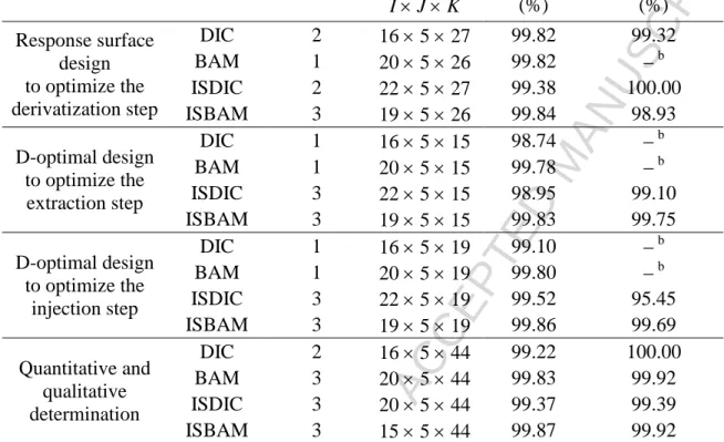
Table 5 shows the characteristics of the models fitted. Two factors were necessary in the PARAFAC2 models for DIC and ISDIC, for BAM a one-factor model was necessary, whereas ISBAM needed three-factors. In all cases the variance explained by the PARAFAC2 models ranged from 99.4 to 99.8%. The CORCONDIA index was always greater than 98.9%, which indicated that the trilinearity hypothesis was assumable in all the cases.
As an example, Fig. 2 shows the loadings of chromatographic, spectral and sample modes obtained for DIC (the loadings of the chromatographic mode in PARAFAC2 models are referred throughout the paper to loadings scaled by the last mode loadings [38]). In this case, the model with two factors explained a 99.8% of variance and had a CORCONDIA index equal to 99.3. The spectral loadings of the second factor were coherent with DIC. For the unequivocal identification, the ratios of the loadings of the spectral profile of 4 diagnostic ions were calculated (expressed as a percentage of the loading of each ion with respect to the highest loading, which corresponds to the base peak); they are shown in Table 4 (5th column). Then, the ratios were checked to see if they were within the tolerance intervals established for the relative ion abundances with respect to a “standard” according to the document SANCO/12495/2011 (at least three ratios or relative ion abundances must be within the tolerance intervals when working with a standard mass resolution detector in the SIM mode for analytes for which a MRL has been established).
ACCEPTED MANUSCRIPT
first factor, related to another compound with shared ions. It was also confirmed that the relative retention times were within the tolerance intervals for the rest of compounds under study. Therefore, spectral and chromatographic profiles matched those of the reference standards and the analytes and internal standards were unequivocally identified in all cases.
Similarly, the second factor of the sample profile in Fig. 2c follows the expected pattern for DIC. The loadings of the last six samples (the six standards) increase with the concentration of DIC. The first of these six samples (sample 22, with 0 μg L−1 of DIC) and the two previous samples (samples 20 and 21, blank onions) have negligible loadings since no DIC was present in them (this confirms that this factor is solely related to DIC). The first 19 samples in Fig. 2c show the distribution of the loadings for the experiments of the central composite design. On the other hand, the loadings of the first factor have similar values both in onion extracts and standards (just prepared in ethyl acetate), so this factor is probably related to some silylation artifact.
As different volumes of BSTFA (VBSTFA) were added to the reconstituted extracts following the experimental plan, the sample loadings had to be corrected by the volume, and these corrected loadings were the responses of the experimental design showed in Table 1. These responses were used to fit the model of Eq. (12) for the four compounds (although the term x2x3 had to be excluded of the models for BAM and ISBAM in order to obtain significant
regression surfaces). Experiment 12 was outlier for BAM and ISBAM; after its elimination, the maximum of the variance inflation factors (VIFs) of the coefficients of these two models was just increased from 1.03 to 1.25 (very close to 1 too, which guaranteed precise estimates for the coefficients of the model). Table 6 shows the parameters and the statistics of the models fitted for the four compounds (experiments 12 and 14 were also excluded from the models of DIC and ISDIC in order to consider the same experimental domain for the four analytes). The analysis of the variance, Section 2.2.1, allows one to affirm that the fitted models explained significantly at a 5% the experimental responses (p-values < 0.05). There was not evidence of lack of fit (p-values > 0.05) at a significance level of 5% in any case. The coefficients of determination ranged from 0.778 to 0.847.
In order to study the response surfaces fitted, as it has been indicated in Section 2.2.1, a study of the optimum path was carried out. Fig. 3 shows the study of the optimum path for DIC (Fig. 3a) and BAM (Fig. 3b); the radius R in abscissas (distance from the center of the design) and the yˆmax(R) in ordinates. The optimum path of the responses shows that the maximum response is reached at the boundary of the experimental domain in both cases, at distances R 1.7 from the center of the experimental design. Ordinate axis in Figs. 3c and 3d has the values x1, x2 and x3 of experimental factors, in coded variables, which define each
ACCEPTED MANUSCRIPT
For example, the analysis of Fig. 3c for values of R 1.7 shows that the maximization of the response for DIC is highly sensitive to the variation of the temperature of the water bath and of the volume of derivatization reagent, and practically insensitive to variations in the derivatization time. That is, to reach the maximum of the response, the temperature of the water bath has to take the lowest value analysed, the volume of derivatization reagent an intermediate value between the corresponding to the center point and the lowest value analysed in the experimental domain, and the derivatization time a value corresponding to the center of the experimental domain. The coordinates for the maximum for DIC, Fig. 3c, transformed into real variables correspond to a derivatization temperature of 42ºC, a volume of derivatization reagent of 44 L, and a derivatization time of 31 min. Similar conditions were found for ISDIC.
On the contrary, the analysis of Fig. 3d shows that the maximization of the response for BAM is highly sensitive to variations in the derivatization time (to reach the maximum value of the response, the derivatization time has to take the highest value analysed), less sensitive to the variation of the temperature of the water bath (it has to take an intermediate value between the highest value analysed and the center of the experimental domain) and practically insensitive to the variation of the volume of derivatization reagent (it has to take a value corresponding to the center of the experimental domain). The coordinates for the maximum, Fig. 3d, transformed into real variables correspond in this case to a derivatization time of 42 min, to a volume of derivatization reagent of 84 L, and to a derivatization temperature of 60ºC. Similar conditions were also found for ISBAM.
These optimum conditions are well different for DIC and BAM, the target analytes, and then it is important to find the compromise optimum, in this case using the Derringer desirability function, as it has been described in Section 2.2.2. In both cases, the individual desirability function was defined in such a way that values higher or equal to 90% of the maximum response were acceptable (desirability 1), whereas values lower than 60% of the maximum response found were unacceptable (desirability 0). In this way, the threshold values were 17147 and 25720 for DIC, and 15226 and 22839 for BAM, respectively. For values of the responses between the threshold values, the individual desirability function ,di, varies linearly
between 0 and 1. To obtain the overall desirability function, d in Eq. (8), p1 = p2 = 1 were set,
which means that the two individual desirability functions were equally weighted. The maximum of the overall desirability function was found for a temperature of 44.65ºC, a time of 43 min, and a volume of BSTFA of 56 L. This solution fulfils the specifications imposed and reaches an overall and individual desirability of 1.
ACCEPTED MANUSCRIPT
experimental domain it is reduced to a circle as small as far is the fixed value of the domain center. The analysis of the desirability function only is valid in that circle that is different for each parameter fixed as can be seen in Fig. 4 d), e) y f). A study of the sensitivity if this maximum to variations in the derivatization conditions shows that variations of a 10% of codified variables around the optimum leads to individual desirabilities between 0.8 and 1, which points out the stability of the optimum found.
Instead of the optimum derivatization time found, 43 min, this factor was fixed at 42 min, because run 12 in Table 1 was considered as outlier, and it is mandatory to avoid extrapolations outside the experimental domain. In these conditions the overall desirability is 1, as for the optimum of 43 min found.
4.3 Optimization of the extraction and clean-up step: first D-optimal design
Table 2 shows the experimental plan and the levels considered for the seven experimental factors studied. The low level of each variable corresponds to the lowest values in Table 2, whereas the highest values correspond to the high level. All coefficients of the model of Eq. (13) were estimated by least squares.
Pretreatments were performed according to this experimental plan on blank onions fortified with 50 g kg-1 of each compound, and next the 12 extracts were derivatized in the optimum conditions found in Section 4.2 and injected into the gas chromatograph. Table 2 also contains the responses of the design, which are the loadings of the sample mode calculated through PARAFAC2 models obtained from the decomposition of the corresponding data tensors (unimodality and negativity constrains in the chromatographic mode and non-negativity constraint in spectral and sample modes were imposed). For obtaining those responses, the GC-MS data from injections of the D-optimal experiments were arranged analogously to that in Section 4.2 in four data tensors, together with the data of 3 standards (containing 30, 50 and 70 μg L−1 of DIC, BAM, ISDIC and ISBAM, in ethyl acetate) which were included to achieve more precise estimations of the three-way models. The size of the data tensors and the characteristics of the PARAFAC2 models are shown in Table 5.
ACCEPTED MANUSCRIPT
mode (Fig. 5c) of the last three samples (the standards) increase with the concentration of BAM as expected, and the rest of the loadings are the responses of the D-optimal design for this analyte shown in Table 2.
The loadings of the four analytes were used in each case to fit the model of Eq. (13), the term
67x x 6 7
β had to be excluded of the model of BAM to fit a significant regression model. Run 2
was outlier in the model fitted for DIC and run 4 in the models fitted for BAM and ISBAM, so both experiments were removed of the corresponding models. The VIFs of the coefficients of those models were between 1.06 and 1.14 after the elimination of outliers, and between 1.04 and 1.14 when the interaction term was also eliminated, so the good quality of estimations is not lost. The fitted models were acceptable because its coefficients of determination ranged from 0.957 to 0.998 and all of them were significant at 5% and did not have lack of fit at a 5% significance level.
Fig. 6 shows the graphic study of the effects of the different pretreatment conditions on the standardized loadings of the sample mode of the four analytes. The significant effects (in light orange) nearly follow the same pattern in all the cases. They were significant in some cases the temperature and time of evaporation (coefficients of Tevap and tevap, i.e. 6 and 7),
together with the times of the vortex mixing steps (coefficients of tmix1 and tmix2, i.e. 1 and 4)
and of the centrifugation steps (coefficients of tcentr1 and tcentr2, i.e. 2 and 5). Alternative
analyses of the effects (graphs of normality and Bayesian approach [25]) show these coefficients to be significant too. The centrifugation speed (coefficient of scentr1, i.e. 3) as
well as the interaction between temperature and time of evaporation (67), had no significant
influence on the responses in the experimental domain studied.
The bars show the coefficients estimated in Eq. (13); their interpretation is as follows: for
4.4 Optimization of the injection step: second D-optimal design
ACCEPTED MANUSCRIPT
A blank onion fortified with 50 g kg-1 of the four analytes was extracted and derivatized using the procedures optimized above. Next the extract was injected into the chromatographic system according to the experimental plan in Table 3. The GC-MS data were acquired for the 16 experiments of the design and for 3 standards which contained 30, 50 and 70 μg L−1 of DIC, BAM, ISDIC and ISBAM in ethyl acetate. The signals were arranged in four data tensors that were decomposed using a PARAFAC2 model (details about the data tensors and the three-linear models are shown in Table 5) in order to obtain the responses of the design i.e. the loadings of the sample mode shown in Table 3.
The PARAFAC2 models had the same number of factors for the four compounds than in the previous study (Section 4.3), since similar interferences on the signals were expected in both cases because the experimental procedure was similar (fortified onion samples were extracted, derivatized, evaporated and reconstituted with ethyl acetate to be injected into the chromatograph). More than 99.10% of the variance was explained always. In all cases the analytes were unequivocally identified according to Document SANCO/12495/2011 as previously (Table 4, 7th column).
As an example, Fig. 7 shows the loadings obtained with the three-factor PARAFAC2 model for ISDIC. The third factor was unequivocally identified as ISDIC through the loadings of the chromatographic and spectral modes of Fig. 7a and b as above. The first and second factors were related to interferents from the matrix, as can be seen in the loadings of the sample mode shown in Fig. 7c; both factors were practically not significant for standards (samples 17, 18 and 19) but only for the experiments of the D-optimal design that corresponded to different injections of an extract of onion.
The loadings of the first 16 samples of the third factor in Fig. 7c were the responses of the experimental design (samples 9 to 12 are replicates) for ISDIC; together with the loadings obtained for the rest of analytes, they were used to fit the model of Eq. (14). The four models fit were significant at 5% level and did not have lack of fit a 5% significance level. In this case, the coefficients of determination were between 0.948 and 0.995. As it has been mentioned above, Section 2.2.3, the coefficients of the reference-state model were estimated by least squares and depend on the reference state chosen; as this can make difficult the interpretation of the effects, to avoid this issue the presence-absence model of Eq. (15) was fitted.
ACCEPTED MANUSCRIPT
Vent flow rate (ventflow or x4), solvent vent time (venttime or x5) and PTV ramp rate (rPTV or x6)
were always significant. In all the cases the coefficients for both ventflow and venttime had a
positive sign for level A, which means that the highest responses were obtained when injection was performed at level A of these factors, 100 mL min-1 and 0.3 min respectively. On the contrary, the coefficient of rPTV had a positive sign for level B, i.e. the highest responses were achieved when this factor was set at 10 ºC s-1. The rest of factors were only significant for BAM and/or ISBAM (except TPTVend, x7, which was never significant). In the
case of the injection speed (sinj,i.e. x8), the intermediate level gave the best responses. The
plot shows that the effect of the injection speed is nonlinear; this could not have been seen if only two levels had been studied.
In the end, taking into account all the effects, the optimized conditions for optimization were:
TPTVinit = 40 ºC, tPTVinit = 0.5 min, Pinit = 9 psi, ventflow = 100 mL min-1, venttime = 0.3 min, rPTV
= 10 ºC s-1, TPTVend = 280 ºC and sinj = 50 L s-1.
4.5 Determination of DIC and BAM in onions
In the optimized conditions, the analysis of DIC and BAM in onions was performed. Eight onion samples (test) of diverse cultivars (white, grain, sweet, “reina chata”,…) purchased in different food stores were analysed twice (all the steps of the experimental procedure were repeated). A common approach used for calibration in the analysis of complex matrices is to prepare the calibration standards in blank matrix and to subject the calibration standards to the entire pretreatment that is used for the test samples; these standards are known as matrix-matched standards. European guidelines recommend the use of matrix-matrix-matched standards to minimize errors related to enhancement/diminishment of the response induced by matrix effects [42], so a matrix-matched calibration was carried out.
Together with the test set, a set of 15 matrix-matched standards (from 0 to 35 g L-1 of DIC and BAM) and a set of 7 samples for recovery studies (a blank sample and 6 samples of onion fortified with 20 μg L−1 of DIC and BAM) were analysed. In all these cases, a concentration of 20 g L-1 was set for the internal standards, ISDIC and ISBAM. In addition, a set of 6 standards (containing 5, 10, 20, 30, 40 and 50 μg L−1 of DIC, BAM, ISDIC and ISBAM in ethyl acetate) was measured and included in the data tensor as above. Therefore, a data tensor of dimension I544 was obtained for the chromatographic peak of each compound after base line correction (the values of I are detailed in Table 5). The first 15 objects corresponded to the matrix-matched standards, the next 7 objects to the samples for recovery studies (the first one was a blank sample), the next 16 objects to the 8 onion samples analysed in duplicate, and the last 6 objects to the standards.
ACCEPTED MANUSCRIPT
models built for DIC and BAM had higher number of factors than the previously obtained models. This was because of the fact that onions of different varieties and origins were included in the dataset, so more different interferents were also included in the analysis. By way of example, Figure 9 shows the estimated loadings of the three-factor model calculated for BAM; in the previous cases a one-factor model was obtained.
The 3rd factor was unequivocally identified with BAM as above through the loadings of the chromatographic and spectral modes (Figs. 9a and 9b, and Table 4). Whereas the other two factors were related to compounds of which the chromatographic peaks appeared on the right (1st factor, blue continuous line) and on the left (2nd factor, green dashed line) of the peak of BAM (the second one was more overlapped with it) in Fig. 9a. Although the severe interference of these other compounds on the diagnostic ions of BAM (Fig. 9b), the PARAFAC2 model has been capable of successfully extracting the contribution of BAM to the signal in the 3rd factor. That is, the second-order advantage of the PARAFAC2 model allowed the determination of BAM in those samples where unknown interferents were present without being necessary to calibrate them. Moreover, if a three-way method did not have been used, the unequivocal identification of BAM could not have been performed according to regulations because matrix interferents contributed a lot to three of the five diagnostic ions of BAM (Fig. 9b), i.e. the diagnostic ions (their relative abundances) would probably not have been verified the compliance.
The loadings of the sample mode (Fig. 9c) also show that the 1st and 2nd factors (blue points and green triangles, respectively) were related basically to the tests samples (samples 23 to 38) because neither for standards or matrix-matched standards they were significant. In fact, the 1st factor (blue points) was related to four concrete samples (samples 25, 26, 37 and 38 in Fig. 9c); which were replicated measurements of two test samples. Those samples also corresponded to the four clear chromatographic peaks of the 1st factor in Fig. 9a, that confirm the fact that the 1st factor was related to some compound which was only present in both onion samples.
Fig. 9c shows that the loadings of the sample mode of the 3rd factor (in squares) followed the pattern expected for BAM; the higher the concentration of BAM in standards and matrix-matched standards the higher the loadings estimated, whereas the loadings for the standards with no BAM (samples 1 and 16) or for the test samples were practically zero.
ACCEPTED MANUSCRIPT
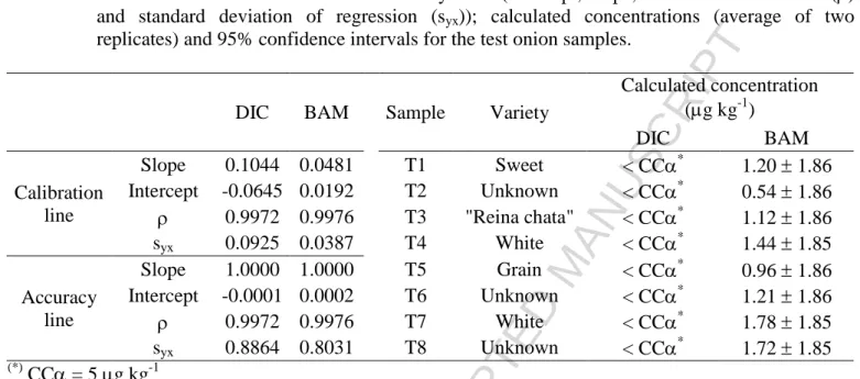
In the regression model fitted for BAM, an outlier (standard of 0.5 g L-1) was detected using the least median of squares (LMS) regression and removed because the absolute value of standardized residual was higher than 2.5, so a reweighted least squares (RLS) regression model was fitted with the rest of data. Table 7 shows the parameters of this regression model, which was suitably validated. The mean of the absolute value of the relative errors in calibration was 6.50%. The concentrations calculated for the eight onion test samples (Table 7) shows that no residues of BAM were found since no significant concentration values were achieved.
For DIC, a calibration line with high relative errors in the calculated concentrations (from -35 to 265%) for the lowest concentrations was obtained when the 15 matrix-matched standards were taken into account. Then, a regression model was fitted with the matrix-matched standards from 0 to 5 g L-1 and it was not significant (p-value = 0.070) at a significance level of 5%, which meant that there was not a linear relation between the standardized loadings and the concentration in this concentration range. So a calibration line was fitted with the matrix-matched standards from 5 to 35 g L-1. Two outliers (standards of 6 and 15
g L-1) were detected and removed; Table 7 shows the parameters of the RLS regression model. In this case, the p-value for the test on significance of the regression was less than 5 10-5, thus the calibration model was significant at a significance level of 0.05. The calculated concentrations of DIC for the test samples are seen in Table 7; none of them was non-compliant, i.e. the MRL was exceeded in no case. The mean of the absolute value of the relative errors in calibration was 4.62%.
Some figures of merit of the optimized procedure were calculated according to that indicated in Section 2.3. The parameters of the accuracy lines are shown in Table 7. Fig. 10 shows the joint confidence estimated regions for slope and intercept; both regions included 1 and 0 respectively, so the trueness was guaranteed for the analysis of both compounds although the analysis of DIC was a little less precise (the dotted ellipse was wider). The standard deviation of these regressions (syx), i.e. the intermediate repeatability in the analysed concentration
range was 0.89 g L-1 for DIC and 0.80 g L-1 for BAM.
Recovery was calculated from the 7 fortified onion samples (samples 16 to 22 in Fig. 9c, for BAM). The first was a blank sample and the next 6 samples were onion samples fortified to contain 20 g L-1 of DIC and BAM. The recovery rates found for DIC and BAM was 92.71 and 97.75% respectively. The repeatability of the analytical procedure was calculated as the standard deviation of the concentration calculated for those 6 fortified samples; values of repeatability of 0.75 g L-1 for DIC and 1.27 g L-1 for BAM were obtained.
For the studied procedure, decision limits at zero (x0 = 0 g kg-1) were 5.00 g kg-1 for DIC
and 1.55 g kg-1 for BAM. And the decision limit at the MRL (x0 = 20 g kg-1) were 21.38
ACCEPTED MANUSCRIPT
for BAM, the analysis was made analogous to that of DIC. In both cases, was equal to 0.05. The value of 5.00 g kg-1 was taken as CC for DIC (which corresponded to the lowest matrix-matched standard of the calibration line) because the value calculated was below the calibration range. That is, the optimized procedure allowed the determination of a minimum of 5.00 g kg-1 of DIC and 1.55 g kg-1 of BAM, values that were well below the MRL established for DIC. Detection capabilities at zero were 5.37 g kg-1 for DIC and 3.03 g kg-1 for BAM, and detection capabilities at the MRL were 23.53 g kg-1 and 22.95 g kg-1 for DIC and BAM respectively. In both cases for = 0.05.
5. Conclusions
Using the experimental design methodology in the optimizations steps made it possible to study the effect of a large number of experimental variables (18 experimental factors in all) on different responses with a reduced number of experiments. The use of the D-optimal designs reduced significantly the number of experiments from 128 to 10 (a 92% reduction) in the optimization of the extraction and cleaning step and from 384 to 13 (almost a 97% reduction) in the optimization of the injection step; while maintaining the quality of estimates. Using the desirability function made it possible to solve the conflict between the optimization of different responses.
The combination of PARAFAC2 modeling and experimental design methodology is a powerful tool in the optimization of procedures in the analysis of complex matrices because of the second-order advantage of PARAFAC2. Without this property, an experimental calibration would have been necessary at each experimental condition studied for each analyte, i.e. 38 calibrations versus the 3 calibration performed in this work. In addition, the unequivocal identification of the analytes could not have been performed according to regulations because they shared diagnostic ions with coeluent derivatization artifacts and matrix interferents, in such a way that their relative abundances would probably not have been verified the compliance.
The analytical procedure optimized in this work allows the determination of DIC and BAM in onions at levels below the MRL established for DIC in this commodity.
6. Acknowledgements
ACCEPTED MANUSCRIPT
Table 1 Experimental plan and responses (loadings of the sample mode of the PARAFAC2 models) for the optimization of the derivatization step.
Run
Experimental plan Responses (loadings)
Temperature Time VBSTFA
DIC BAM ISDIC ISBAM
(ºC) (min) (L)
1 48 18 36 23233 16420 24795 13697
2 72 18 36 16079 18176 18060 15061
3 48 42 36 24347 20958 25965 20132
4 72 42 36 15878 18051 18448 15232
5 48 18 84 17595 16714 20885 15879
6 72 18 84 25801 21603 28329 19715
7 48 42 84 21615 21734 23823 20982
8 72 42 84 25904 25377 28128 22335
9 40 30 60 28578 18232 31071 17267
10 80 30 60 18617 18501 21441 14089
11 60 10 60 18477 20617 21179 19803
12 60 50 60 16387 18424 18753 19598
13 60 30 20 15891 14354 18159 12575
14 60 30 100 24028 27230
15 60 30 60 17598 16427 19383 15685
16 60 30 60 21947 20190 23709 19661
17 60 30 60 21651 21501 22517 21298
18 60 30 60 19656 17633 20825 16562
ACCEPTED MANUSCRIPT
Table 2 Experimental plan and responses (loadings of the sample mode of the PARAFAC2 models) for the optimization of the extraction and clean-up procedure. Factors: time of the 1st vortex mixing step (tmix1); time and rotational speed of the 1st centrifugation step (tcentr1 and scentr1); time of the 2st vortex mixing step (tmix2); time of the 2nd centrifugation step (tcentr2);
and temperature and time of evaporation (Tevap and tevap).
Run
Experimental plan Responses (loadings)
tmix1 tcentr1 scentr1 tmix2 tcentr2 Tevap tevap
DIC BAM ISDIC ISBAM
(min) (min) (rpm) (s) (min) (ºC) (min)
1 1 10 6000 30 1 40 10 10856 13984 10109 13469
2 2 5 3000 60 5 40 10 6083 10548 5518 10251
3 2 5 3000 60 5 40 10 9027 11878 7376 11098
4 2 5 3000 60 5 40 10 8845 13270 7009 13379
5 2 5 3000 30 1 50 10 10742 15249 8319 14232
6 1 10 3000 60 5 50 10 10020 14058 8245 13127
7 2 5 6000 60 5 50 10 9540 12082 7178 11544
8 2 10 3000 60 1 40 15 6697 13305 3850 12605
9 1 5 6000 30 5 40 15 5863 9965 3564 9066
10 1 5 3000 60 1 50 15 5385 13258 2347 12523
11 2 10 6000 60 1 50 15 8470 15627 4731 15354
ACCEPTED MANUSCRIPT
Table 3 Experimental plan and responses (loadings of the sample mode of the PARAFAC2 models) for the injection step. Factors: PTV initial temperature and pressure (TPTVinit and tPTVinit); initial column head pressure (Pinit); vent flow rate (ventflow); solvent vent time (venttime); PTV ramp rate and final temperature (rPTV andTPTVend); and injection speed (sinj).
Run
Experimental plan Responses (loadings)
TPTVinit tPTVinit Pinit ventflow venttime rPTV TPTVend sinj
DIC BAM ISDIC ISBAM
(ºC) (min) (psi) (mL min-1) (min) (ºC s-1) (ºC) (L s-1)
1 40 0.6 8.1 150 0.45 5 260 1 2411 3856 1947 4078
2 50 0.5 9.1 150 0.45 10 260 1 7008 8299 7718 6900
3 40 0.6 8.1 100 0.3 10 260 1 8925 12805 7943 11657
4 50 0.5 8.1 100 0.45 5 280 1 3190 6654 2522 4601
5 50 0.6 9.1 100 0.3 5 280 1 3002 6740 2381 5697
6 40 0.5 9.1 150 0.3 10 280 1 11585 13911 12090 12856
7 40 0.5 9.1 100 0.45 5 260 50 5086 12174 3800 10778
8 50 0.6 9.1 150 0.3 5 260 50 2078 6954 1615 5250
9 40 0.5 8.1 100 0.3 10 280 50 16745 14094 16414 13778
10 40 0.5 8.1 100 0.3 10 280 50 17132 15061 16684 14456
11 40 0.5 8.1 100 0.3 10 280 50 17953 15659 17922 15000
12 40 0.5 8.1 100 0.3 10 280 50 18839 13590 18781 13741
13 50 0.6 8.1 150 0.45 10 280 50 3813 5739 4082 4166
14 50 0.5 8.1 150 0.3 5 260 100 2650 8027 2112 5733
15 50 0.6 9.1 100 0.45 10 260 100 5368 8800 5816 7016
ACCEPTED MANUSCRIPT
Table 4 Detected ions (the most base peaks are in bold), relative abundances and tolerance intervals calculated from the PARAFAC2 models estimated from the data tensors including the 7 reference standards, and relative abundances calculated with the loadings of the spectral profiles of the PARAFAC2 models estimated in the optimization of derivatization, of extraction and of injection steps, and in the quantitative and qualitative determination step.
ACCEPTED MANUSCRIPT
Table 6 Statistics and parameters of the response surface models fitted for the optimization of the derivatization step. Significance of the regression and lack of fit mean the p-values of the significance of the regression and lack of fit tests performed for validating the regression models. R2 is the coefficient of determination. Coefficients b0 to b23 are the coefficients of the models fitted.
DIC BAM ISDIC ISBAM
Significance of the regressiona 0.037 0.048 0.033 0.043
Lack of fitb 0.199 0.845 0.205 0.900
Null hypothesis: the linear model is not significant
(b)
Null hypothesis: the regression model adequately fits the data
(*)
ACCEPTED MANUSCRIPT
32/49
Table 7 Parameters of the calibration and accuracy lines (intercept, slope, correlation coefficient () and standard deviation of regression (syx)); calculated concentrations (average of two
replicates) and 95% confidence intervals for the test onion samples.
DIC BAM Sample Variety
Calculated concentration (g kg-1)
DIC BAM
Calibration line
Slope 0.1044 0.0481 T1 Sweet < CC* 1.20 1.86
Intercept -0.0645 0.0192 T2 Unknown < CC* 0.54 1.86
0.9972 0.9976 T3 "Reina chata" < CC* 1.12 1.86
syx 0.0925 0.0387 T4 White < CC* 1.44 1.85
Accuracy line
Slope 1.0000 1.0000 T5 Grain < CC* 0.96 1.86
Intercept -0.0001 0.0002 T6 Unknown < CC* 1.21 1.86
0.9972 0.9976 T7 White < CC* 1.78 1.85
syx 0.8864 0.8031 T8 Unknown < CC* 1.72 1.85
(*)
ACCEPTED MANUSCRIPT
33/49 Highlights
Determination of dichlobenil and BAM in onions by PTV-GC-MS according to SANCO 12495
Derivatization, extraction and PTV injection optimization with experimental designs
Combination of experimental design methodology and PARAFAC2 models, a powerful tool.