The ESSENCE supernova survey: Survey optimization, observations, and supernova photometry

Texto completo

(1)Submitted to ApJ on December 7, 2006. arXiv:astro-ph/0701043v1 2 Jan 2007. The ESSENCE Supernova Survey: Survey Optimization, Observations, and Supernova Photometry G. Miknaitis1 , G. Pignata2 , A. Rest3 , W. M. Wood-Vasey4 , S. Blondin4 , P. Challis4 , R. C. Smith3 , C. W. Stubbs4,5 , N. B. Suntzeff3,6 , R. J. Foley7 , T. Matheson8 , J. L. Tonry9 , C. Aguilera3 , J. W. Blackman10 , A. C. Becker11 , A. Clocchiatti2 , R. Covarrubias11 , T. M. Davis12 , A. V. Filippenko7 , A. Garg4,5, P. M. Garnavich13 , M. Hicken4,5 , S. Jha7,13 , K. Krisciunas13,6 , R. P. Kirshner4 , B. Leibundgut14 , W. Li7 , A. Miceli11 , G. Narayan4,5 , J. L. Prieto15 , A. G. Riess16,17 , M. E. Salvo10 , B. P. Schmidt10 , J. Sollerman12,18 , J. Spyromilio14 , A. Zenteno3 [email protected].

(2) –2– ABSTRACT We describe the implementation and optimization of the ESSENCE supernova survey, which we have undertaken to measure the equation of state parameter of the dark energy. We present a method for optimizing the survey exposure times and cadence to maximize our sensitivity to the dark energy equation of state parameter w = P/ρc2 for a given fixed amount of telescope time. For our survey on the CTIO 4m telescope, measuring the luminosity distances and redshifts for 1. Fermi National Accelerator Laboratory, P.O. Box 500, Batavia, IL 60510-0500. 2. Pontificia Universidad Católica de Chile, Departamento de Astronomı́a y Astrofı́sica, Casilla 306, Santiago 22, Chile 3. Cerro Tololo Inter-American Observatory, National Optical Astronomy Observatory, Casilla 603, La Serena, Chile 4. Harvard-Smithsonian Center for Astrophysics, 60 Garden Street, Cambridge, MA 02138. 5. Department of Physics, Harvard University, 17 Oxford Street, Cambridge, MA 02138. 7. Department of Astronomy, 601 Campbell Hall, University of California, Berkeley, CA 94720-3411. 8. National Optical Astronomy Observatory, 950 North Cherry Avenue, Tucson, AZ 85719-4933. 9. Institute for Astronomy, University of Hawaii, 2680 Woodlawn Drive, Honolulu, HI 96822. 10. The Research School of Astronomy and Astrophysics, The Australian National University, Mount Stromlo and Siding Spring Observatories, via Cotter Road, Weston Creek, PO 2611, Australia 11. Department of Astronomy, University of Washington, Box 351580, Seattle, WA 98195-1580. 12. Dark Cosmology Centre, Niels Bohr Institute, University of Copenhagen, Juliane Maries Vej 30, DK-2100 Copenhagen Ø, Denmark 13. Department of Physics, University of Notre Dame, 225 Nieuwland Science Hall, Notre Dame, IN 465565670 13. Kavli Institute for Particle Astrophysics and Cosmology, Stanford Linear Accelerator Center, 2575 Sand Hill Road, MS 29, Menlo Park, CA 94720 6 14. Department of Physics, Texas A&M University, College Station, TX 77843-4242 European Southern Observatory, Karl-Schwarzschild-Strasse 2, D-85748 Garching, Germany. 15. Department of Astronomy, Ohio State University, 4055 McPherson Laboratory, 140 West 18th Avenue, Columbus, OH 43210 16. Space Telescope Science Institute, 3700 San Martin Drive, Baltimore, MD 21218. 17. Johns Hopkins University, 3400 North Charles Street, Baltimore, MD 21218. 18. Department of Astronomy, Stockholm University, AlbaNova, 10691 Stockholm, Sweden.

(3) –3– supernovae at modest redshifts (z ∼ 0.5 ± 0.2) is optimal for determining w. We describe the data analysis pipeline based on using reliable and robust image subtraction to find supernovae automatically and in near real-time. Since making cosmological inferences with supernovae relies crucially on accurate measurement of their brightnesses, we describe our efforts to establish a thorough calibration of the CTIO 4m natural photometric system. In its first four years, ESSENCE has discovered and spectroscopically confirmed 102 type Ia SNe, at redshifts from 0.10 to 0.78, identified through an impartial, effective methodology for spectroscopic classification and redshift determination. We present the resulting light curves for the all type Ia supernovae found by ESSENCE and used in our measurement of w, presented in Wood-Vasey et al. (2007). Subject headings: cosmology: observations — supernovae — surveys — methods: data analysis. 1.. Introduction. This is a report on the first four years of the ESSENCE survey (Equation of State: SupErNovae trace Cosmic Expansion), a program to measure the cosmic equation of state parameter to a precision of 10% through the discovery and monitoring of high redshift supernovae. The motivations and goals of ESSENCE, as well as the methods and data are presented here. ESSENCE is part of the exploration of the new and surprising picture of an accelerating universe, which has become the prevailing cosmological paradigm. This paradigm is supported by essentially all current observations, including those based on supernova distances, the large scale clustering of matter, and fluctuations in the cosmic microwave background. The free parameters of this concordance model can consistently fit these diverse and increasingly precise measurements. This paper describes the survey design and optimization, and the acquisition and photometric analysis of our data through to the generation of photometrically calibrated SN light curves. The companion paper by Wood-Vasey et al. (2007) describes how luminosity distances are measured from the SN light curves and derives constraints on w from the ESSENCE observations..

(4) –4– 1.1.. Cosmology and Dark Energy. While the current observational agreement on a concordance model is surprisingly good (Tegmark et al. 2004; Eisenstein et al. 2005; Spergel et al. 2006), it comes at the high cost of introducing two unknown forms of mass-energy: non-baryonic dark matter and dark energy that exerts negative pressure. Each is a radical idea, and it is only because multiple independent observations require their existence that we have come to seriously consider new physics to account for these astronomical phenomena. The dark energy problem is currently one of the most challenging issues in the physical sciences. The stark difference between the staggeringly large value for the vacuum energy predicted by quantum field theory and the cosmic vacuum energy density inferred from observations leads us to wonder how this vacuum energy of the Universe could be so small (Weinberg 1989; Carroll et al. 1992; Padmanabhan 2003; Peebles & Ratra 2003). On the other hand the convergence of observations that give rise to the ΛCDM concordance cosmology, with ΩΛ ∼ 0.7 rather than identically zero, forces us to ask why the vacuum energy is so large. More broadly, these cosmological observations can be interpreted as evidence for physics beyond our standard models of gravitation and quantum field theory. It is perhaps no coincidence that this occurs at the friction point between these two independently successful, but as yet unmerged paradigms. Our understanding of the gravitational implications of quantum processes appears to be incomplete at some level. The dark energy problem challenges us on many fronts: theoretical, observational and experimental. Observational cosmology has an important role to play, and the current challenge is to undertake measurements that will lead to a better understanding of the nature of the dark energy (Albrecht et al. 2006). In particular we seek to measure the equation of state parameter w = P/ρc2 of the dark energy, as this can help us test theoretical models. One specific goal is to establish whether the observed accelerating expansion of the Universe is due to a classical cosmological constant or some other new physical process. Within the framework of Friedmann-Robertson-Walker cosmology, the only way to reconcile the observed geometric flatness and the observed matter density is through another component of mass-energy that does not clump with matter. The observation of acceleration from supernovae is the unique clue that indicates this component must have negative pressure (Riess et al. 1998; Perlmutter et al. 1999; Riess et al. 2001; Tonry et al. 2003; Knop et al. 2003; Barris et al. 2004; Riess et al. 2004; Clocchiatti et al. 2006; Astier et al. 2006; Riess et al. 2006). As the evidence from supernovae has grown more conclusive, the intellectual focus has shifted from verifying the existence of dark energy to constraining its.

(5) –5– properties (Freedman & Turner 2003). Accordingly, several large-scale, multi-year supernova surveys have embarked on studying dark energy by collecting large, homogenous data sets. The Supernova Legacy Survey has published cosmological constraints using 73 SNe from its first year sample (Astier et al. 2006) between redshifts 0.2 and 1.0, and it continues to accumulate data. More recently, SDSS-II Supernova Survey (Frieman et al. 2004) has observed ∼ 200 supernovae at redshifts out to 0.4. The final supernova samples from each of these programs and ESSENCE will each number in the hundreds. Of the various models for dark energy currently being discussed in the literature, the cosmological constant (i.e. some uniform vacuum energy density) holds a special place, as both the oldest, originating with Einstein, and, in many ways, the simplest (Carroll et al. 1992). Quantum field theory suggests how to calculate the energy of the vacuum, but there is no plausible theoretical argument that accounts for the small, but non-zero, value required by observations. A host of other alternatives has been proposed, many of which appeal to slowly rolling scalar fields, similar to those used to describe inflation. Such models readily produce predictions that agree with the current observational results, but suffer from a lack of clear physical motivation, being concocted after the fact to solve a particular problem. Another class of ideas appeals to higher dimensional “brane world” physics inspired by string theory; for example, the cyclic universe (Steinhardt & Turok 2002, 2005) or modifications to gravity due to the existence of extra dimensions (Dvali et al. 2003). One straightforward way to parameterize the dark energy is by assuming its equation of state takes the form P = wρc2 , where P and ρ are pressure and density respectively, related by an “equation-of-state” parameter w. Non-relativistic matter has w = 0, while radiation has w = +1/3, and different proposed explanations for the dark energy have a variety of values of w. In general, to produce an accelerated expansion, a candidate dark energy model must have w < −1/2 for a current matter density of ΩM ∼ 1/3. The classical cosmological constant, Λ, of General Relativity has an equation-of-state parameter w = −1 exactly, at all times. Other models can take on a variety of effective w values that may vary with time. For example, quintessence (Steinhardt 2003) posits a minimally coupled rolling scalar field, with an equation of state, 1 2 φ̇ − V (φ) P w∼ = 21 . (1) 2 + V (φ) ρ φ̇ 2 In this case, the effective value of w depends on the form of the potential chosen and can evolve over time. In general the parameterization of dark energy in terms of w is a convenient and useful tool to compare a variety of models (Weller & Albrecht 2002). As a first step towards determining the nature of dark energy, the obvious place to start is to test whether the observed w is consistent with −1 (Garnavich et al. 1998). If not, then.

(6) –6– a cosmological constant is ruled out as the explanation for dark energy. If w is measured to be consistent with −1, then while models that exhibit an effective w ∼ −1 are still allowed, the range in parameter space in which they can exist will be significantly restricted. Breaking the degeneracy between Λ and such “impostors” would then require measurements of the additional parameters that describe their time dependence. However, the form of such a parameterization is at present largely unrestricted and the choice of arbitrary parameterizations influences the conclusions derived from the analysis of the data (Upadhye et al. 2005). In the future, measurements of growth of structure, such as through weak lensing surveys, will provide a powerful complement to supernova measurements in constraining the properties of dark energy, as well as checking for possible modifications to General Relativity (Albrecht et al. 2006). In the near term, constraining w under the assumption that it is constant allows us to test a well-posed hypothesis that can be addressed with existing facilities and methods. While under standard General Relativity, w is bounded by the null dominant energy condition to be greater than or equal to −1, we should keep an open mind as to whether the data allow w < −1, since dark energy may well arise from physics beyond today’s standard theories. Motivated by these considerations, we have undertaken a project to use type Ia supernovae to measure w with a target fractional uncertainty of 10%. Observations of type Ia supernovae provided the first direct evidence for accelerating cosmic expansion, and they remain an incisive tool for studying the properties of the dark energy..

(7) –7– 1.2.. Measuring the physics of dark energy with supernovae. Type Ia supernovae (SNe Ia) are among the most energetic stellar explosions in the universe. Their high peak luminosities (4−5×109 L⊙ ) make SNe Ia visible across a large fraction of the observable universe. The peak luminosity can be calibrated to ∼ 15% precision in flux (Phillips 1993; Hamuy et al. 1996; Riess et al. 1996; Goldhaber et al. 2001; Guy et al. 2005; Jha et al. 2007). They are thus well suited to probing the expansion history during the epoch in which the Universe has apparently undergone a transition from deceleration to acceleration (0 < z < 1). The utility of SNe Ia as “standardizable” candles was established observationally by Phillips (1993), with the identification of a correlation between peak luminosity and width of the light curves. The “type Ia” designation is an observational distinction, denoting objects whose spectra lack hydrogen or helium features, but exhibit a characteristic absorption feature observed at λ6150, but attributed to Si ii λ6355. These objects are now thought to be the thermonuclear disruption of a carbon-oxygen white dwarf at or near the Chandrasekhar mass (Hoyle & Fowler 1960), with accretion from a companion star. Material gained through accretion pushes the total mass of the C-O WD above what can be supported by degeneracy pressure and results in nuclear burning, which eventually results in a powerful burning wave that completely destroys the star. A large fraction of the progenitor burns rapidly to produce 56 Ni, whose radioactive decay then powers the observed light curve (Colgate & McKee 1969). Bolometric light curves suggest that ∼ 0.7M⊙ of 56 Ni is produced, which suggests that the burning is incomplete (Contardo et al. 2000; Stritzinger et al. 2006). There is disagreement on important details of whether the burning wave is supersonic (a detonation) or purely subsonic (a deflagration) (Hillebrandt & Niemeyer 2000). Nevertheless, models for the explosion give broad agreement with the observed light curves and spectra, though the specifics of progenitors and explosion physics remain unresolved (Branch et al. 1995; Renzini 1996; Nomoto et al. 2000; Livio 2000). Fortunately, so far the lack of a detailed understanding of supernova physics has not prohibited the use of these objects as probes of cosmology, as the empirical correlations of light curve shape and color with luminosity appear to largely “standardize” supernovae. Subtle effects such as how supernovae are connected to stellar populations and how those populations may change with time and chemical composition will certainly become important in the future as we attempt to place ever tighter constraints on dark energy (Hamuy et al. 2000; Jha 2002; Gallagher et al. 2005; Sullivan et al. 2006). For example, observations suggest that the brightest SNe Ia are found only in galaxies with current star formation. As in classical physics, the flux density from a cosmological source falls off as the inverse.

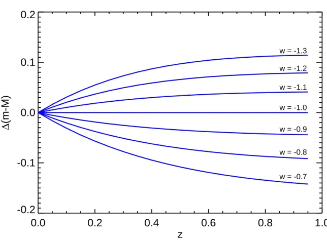
(8) –8– square of distance, F=. L . 4πDl2. (2). However, this luminosity distance, Dl , depends upon how the universe expands as a photon travels from emitter to receiver, which in turn depends sensitively on the composition and properties of the constituents of the cosmic mass-energy density. Specifically, for a flat universe the luminosity distance, Dl (z), is given by c(1 + z) Dl = H0. Z. z 0. 1 p. (1 − ΩM )(1 +. z ′ )3(1+w). + ΩM (1 +. z ′ )3. dz ′ ,. (3). where w is taken here to be constant. In cosmological analyses, the combination of the Hubble constant and the intrinsic luminosity of SNe Ia is a multiplicative nuisance parameter which scales distance measurements at all redshifts by the same amount. Thus, under the assumption of flatness, ΩM +ΩX = 1, when measuring w, the only other free cosmological parameter is the matter density, ΩM . If we seek to constrain w using the luminosity distance-redshift test, it is worth considering which redshifts are most incisive. The relative differences in distance modulus as a function of redshift, for different values of w, are shown in Figure 1, where ΩM and ΩΛ have been fixed at 0.3 and 0.7 respectively. There is a significant w-dependent signal even at intermediate redshifts (z ∼ 0.4), at which observations with a 4-meter class telescope can readily yield many supernovae each month. Of course, observations such as the ESSENCE survey actually produce a complex set of constraints in cosmological parameter space, but much of the signal of interest is readily accessible at intermediate redshifts, between 0.3 and 0.8.. 1.3.. Considerations for optimally constraining w with SNe Ia observations. We wish to determine the optimal use of the time allocated for the ESSENCE survey on the Blanco 4m for constraining w. For a ground-based survey, a variety of factors determine the number of useful supernovae monitored, and the uncertainties associated with each data point on the light curve. The overall quality of each supernova light curve, in turn, determines the precision of its luminosity distance. Some of factors which impact the ability of a particular survey strategy to constrain cosmological parameters include: • Typical site conditions: Seeing, weather, sky background, atmospheric transmission..

(9) –9–. 0.2. w = -1.3. 0.1. w = -1.2. ∆(m-M). w = -1.1 w = -1.0. 0.0. w = -0.9 w = -0.8. -0.1 w = -0.7. -0.2 0.0. 0.2. 0.4. 0.6. 0.8. 1.0. z Fig. 1.— Differences in distance modulus for different values of w as a function of redshift, relative to w = −1, for Ωm = 0.3, ΩΛ = 0.7. Note that even at modest redshifts there is a significant fraction of the total asymptotic signal available. • System throughput vs. wavelength: Aperture, optics, field of view, detector quantum efficiency. • Temporal constraints: Telescope scheduling constraints, camera readout time. • SNR considerations: Requisite S/N ratio and cadence required for distance determination. • Passband considerations: Number of bands needed for extinction and SN color discrimination. • Spectroscopic considerations: Location, availability and scheduling of followup spectroscopic resources.

(10) – 10 – In order to optimize the observational survey strategy for ESSENCE, we tried to parameterize several of the factors above and balance them to obtain the strongest constraints on w. With the strong cosmological signal available in the redshift range from 0.3 to 0.8, it is clear that a wide-field camera on a 4m-class telescope can provide the needed balance of photometric depth (SNe Ia have m∼22 at peak at z=0.5) and sky coverage. Smaller fields of view on larger telescopes are better suited to going to higher redshifts, while wider fields on smaller telescopes are only able to reach redshifts where the cosmological signal is small. Combining these criteria with the range of spectroscopic followup facilities available to our collaboration, we quickly focused our analyses on the Blanco 4m telescope at CTIO together with the MOSAIC camera as providing an optimal combination of site (seeing plus weather), aperture, field of view, and telescope scheduling. Beyond the selection of appropriate telescopes and instrumentation, there are relatively few “free parameters” controllable by the observers. These include the optical passbands used, the exposure time in each passband for each field, the total number of fields monitored, the cadence of the repeated observations, and ability to obtain spectra for each supernova candidate. Using existing knowledge of the distribution of supernova magnitudes and colors as a function of redshift and time after explosion, we can relate the exposure times in different passbands, for a given desired signal-to-noise ratio (SNR). The calibration of luminosity from light curve shape is currently best understood in rest-frame B and V passbands. These passbands map to observer-frame R and I for supernovae at z ∼ 0.4 (i.e. the uncertainties in k-corrections (Nugent et al. 2002) are small). For supernovae at these redshifts, observations taken in R and I, with the I band exposure time equal to twice that in R, are sufficient to match the SNR in both bands and measure distances to the SNe Ia. While observations in a third bandpass would aid in determination of color, and thus, the estimates of extinction in the host galaxies, such observations would require significant additional observing time and are not easily accommodated within our optimization of limited observing time, photometric depth, sky coverage, and number of resulting SNe. Acquiring V band observations would provide a better match to rest-frame B for low redshift supernovae, but supernovae in our sample will be bright and have well-measured colors at these redshifts. Observations in the z-band would aid the color determination at higher redshifts, but the low quantum efficiency of of the MOSAIC CCD detectors, as well as the brightness of the night sky in this band and the heavy fringing due to night-sky emission lines make obtaining useful data in this band impractical. Therefore, by limiting our strategy to R and I and demanding that I band exposure times scale with R band exposure time, the survey optimization problem then is reduced to.

(11) – 11 – considering a single free parameter: the distribution of R band integration times across the survey fields for a given fixed amount of telescope time. What is the balance between survey depth (which extends the redshifts probed) and area (which increases the area covered each redshift slice)? Consider the cosmological information contained in a single, perfect measurement of distance and redshift. Under the assumption of flat geometry (and with perfect knowledge of H0 and the intrinsic luminosity of SNe Ia), each such measurement traces out a curve of allowable values of ΩM and w , as shown in Figure 2. It is clear that if the goal is to measure w from SNe Ia alone, a large span in redshift is desirable in order to maximize the orthogonality of the curves and break the degeneracy between matter density and the equation-of-state parameter. However, because the difference between these curves is small even over a large span in redshift, such a measurement would require massive numbers of SNe Ia achievable only by next generation experiments, such as the DES, PanSTARRS, LSST or JDEM. In the near term, we may appeal to other cosmological measurements to provide a constraint on Ωm , such as from large scale structure measurements. This affords us some freedom in the redshifts at which we make our measurements, since the constraints from distance measurements are nearly orthogonal to an Ωm prior of ∼0.3 at all redshifts. 1 Though the sensitivity to differences in cosmological models is weaker at lower redshifts, there is a powerful observational advantage to working there, because obtaining good photometric and spectroscopic measurements is far cheaper in units of telescope time. To understand the trade-offs between the cosmological sensitivity of samples obtainable under differing observational strategies, we carried out simulations to predict the number and distribution in redshift and magnitude of the set of SNe Ia detectable for survey of a given length and limiting magnitude set by the R-band exposure time. We adopt the methodology used in Tonry et al. (2003) to model the redshift-magnitude distribution of SNe Ia. In brief, we assume the supernovae luminosity function used in Li et al. (2001b), modeled as three distinct luminosity classes representing “normal” , over-luminous (1991T-like) and sub-luminous (1991bg-like) supernovae, each following a Gaussian distribution. This is then convolved with an estimated distribution of extinction due to dust in the supernova host galaxies (Hatano et al. 1998). We can then generate mock supernova samples for various possible survey implementations. For the purposes of survey optimization, it is sufficient to 1. We consider here a prior on Ωm alone, though in reality constraints from measurements of the matter power spectrum, baryon acoustic oscillations or cosmic microwave background produce constraints which have at least mild degeneracy with other cosmological parameters. This simple prior is sufficient for the survey optimization arguments presented here..

(12) – 12 –. -0.5. w. -1.0. -1.5. z=. 0. 0.1. z=1.. -2.0 0.0. 0.2. 0.4 Ωm. 0.6. 0.8. Fig. 2.— Curves in Ωm and w for perfect measurements of distance at redshifts from 0.1 to 1.0, in steps of ∆z = 0.1, for Ωm = 0.3, ΩΛ = 0.7. restrict our considerations to flat cosmologies, neglecting degeneracies with Ωtotal . To estimate the acheivable cosmological constraints, we use an analytic description of how the uncertainty in distance modulus depends on redshift, as the typical signal-tonoise ratio of the photometry decreases at higher redshift, but the temporal sampling (in the SN rest frame) improves due to time dilation. The uncertainty in distance modulus is approximated by the expression: 1.3 δµ (z) = × SNRpeak. r. ∆tobs × 1+z. r. Nobs , Nobs − 3. (4). where ∆tobs gives the time in days between observations, Nobs specifies the number of observations between -10 and +15 days (relative to maximum) in the SN rest frame, and the.

(13) – 13 – Nobs − 3 term arises from three degrees of freedom in the fit of an SN light curve – time of maximum, luminosity at maximum and the width of the light curve. This contribution to the distance uncertainty due to observational constraints is then summed in quadrature with the intrinsic dispersion in type Ia peak luminosities, taken conservatively to be 0.2 magnitudes. With the resulting mock Hubble diagrams, we then can predict the cosmological constraints obtainable for a given survey depth.. 1.4.. The ESSENCE Strategy. This generalized analysis can now be applied to our selected observational system, the Blanco 4m, in order to derive an optimal balance of photometric depth (or equivalently exposure time) and sky coverage given the range of conditions one might expect during a survey using a fixed amount of observing time. We assumed a five year survey with approximately 15 nights per year spread over three months each year. The results are shown in Figure 3. We find that the final achievable uncertainty in w is surprisingly insensitive to the survey depth, with the trade-off between the number of supernovae and the redshifts at which they are found roughly cancelling. There is a weak optimum at tR = 200 seconds because very shallow surveys lose cosmological leverage as the redshift range probed decreases. After initially opting for a range of exposure times designed to match a range of redshift bins covering z = 0.3 − −0.8 in 2002, and finding that the efficiency at shorter exposure times was inadequate, we settled on exposure times of tR = 200 seconds and tI = 400 seconds as the baseline for the rest of the ESSENCE survey..

(14) – 14 – 2.. The ESSENCE Survey 2.1.. Observations. Based on the survey strategy described above, the ESSENCE team submitted a proposal to the NOAO Survey program in 2002. We chose to propose a survey strategy to share time with the ongoing SuperMACHO survey, which uses only half nights on the Blanco telescope. ESSENCE was awarded 30 half nights per year for a five year program (recently extended to six), as well as additional calibration time on the CTIO 0.9m telescope together with some followup time on the WIYN 3.5m telescope. The ESSENCE time is generally scheduled during dark and grey time for three consecutive months, from October to December each year, although the timing of new moons sometimes moves the schedule into September or January. Each month, we observe every other night over a span of 20 days centered on new moon. This schedule leaves approximately ten bright nights each month with no light curve coverage.. 2.1.1. The Instrument ESSENCE survey data are taken using the MOSAIC II imaging camera, which consists of eight 2048x4096 pixel charge-coupled devices (CCDs) arranged in two rows of four, with gaps corresponding to approximately 50 pixels between rows and 35 pixels between columns. In the f/2.87 beam at prime focus, this yields a field of view of 0.6 degrees on a side for a total area of 0.36 square degrees on the sky. The CCDs are thinned back-illuminated silicon devices manufactured by SiTE with 15-um pixels. At the center of the focal plane, each pixel subtends 0.27 arc-seconds on a side, though the pixel scale varies quadratically as a function of radius due to optical aberrations, such that pixels at the corners of the camera subtend a smaller area on the sky by 8%. The CCDs are read out in dual-channel mode, in which the chip is bisected in the long direction and read out in parallel through two separate amplifiers, for a read time of about 100 seconds. Because the amplifiers are not perfectly identical, we treat the sixteen resultant 1048x4096 “amplifier images” as independent data units in our data reduction. All ESSENCE observations are taken through the Atmospheric Dispersion Corrector (ADC), which is composed of two independently rotating prisms that compensate for variation in atmospheric refraction with airmass..

(15) – 15 – 2.1.2. ESSENCE Fields We selected fields that are equatorial, so that they can be accessed by telescopes in the northern and southern hemisphere for followup spectroscopy. The fields are spaced across the sky so that all observations may be taken at low airmass. We chose regions with low Milky Way extinction, for maximum visibility of these faint extra-galactic sources and to minimize systematic error incurred by correcting for extinction due to the Milky Way. Fields with contamination from bright stars, whose large footprint in the imaging data would reduce the effective search area, were avoided. Additional considerations in field selection included a preference for areas with minimal IR cirrus (based on IRAS maps), a preference for areas out of both the galactic and ecliptic planes, and a preference for fields which overlapped previous wide-field surveys (such as the Sloan Digital Sky Survey (SDSS), NOAO Deep Wide-Field Survey, and the Deep Lens Survey). The first ESSENCE observations commenced on 2002 September 28. For this first year of operations, a set of 36 fields was defined. These fields were divided into two sets, which were then observed every other ESSENCE night, resulting in an cadence of every 4 nights on any particular field. This proved to be a challenging inaugural season for the project. The El Niño Pacific weather pattern was in effect, which produced heavy cloud cover much of time, resulting in either lost observing time or data of such poor quality that the detection of faint supernovae was often not possible. Also, the newly commissioned computing cluster experienced catastrophic failure shortly after data collection began, bringing real-time analysis of the data to a standstill for much of that observing campaign. On the night of November 9, the I-band filter sustained significant damage, resulting in a crack. This severely degraded the I band data quality in CCDs 1 and 2 (amplifiers 1-4), resulting in a diminished effective field of view for the rest of the season. This filter was replaced on May, 24, 2003. As described below, many of the 2002 fields have not yet been repeated to provide template images to extract the supernova light curves. The complete analysis of the 2002 data will take place when these reference images are obtained. We provide summary information about the 15 spectroscopically confirmed Ia from this season in Table 3, we only present the light curves for four of these objects for which current reductions are of sufficient quality to merit use in the cosmological analysis in Wood-Vasey et al. (2007). The final ESSENCE supernova sample will include all of the 2002 objects. Observations for the second year of ESSENCE began on September 28, 2003. In order to facilitate scheduling of follow-up observations with the Hubble Space Telescope (HST), which requires advance knowledge of the approximate location of the targets, it was necessary to cluster the search fields together into four groups. The new field set consisted of 32 fields, clustered spatially in sets of eight, such that they were within the pointing error box.

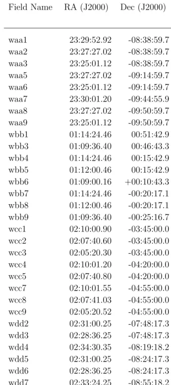
(16) – 16 – of the HST. To the extent possible, fields from 2002 were used as the basis for the new fields. The fields were again divided into two separate sets, observed on alternating nights, providing for an observational cadence of every 4 nights for any given field. In table 1, we list the coordinates of the 32 search fields monitored by ESSENCE from 2003 onward. Results from the subset of nine ESSENCE supernovae observed with HST were presented in Krisciunas et al. (2005)..

(17) – 17 –. Table 1. Coordinates of the centers of the ESSENCE search fields. Field Name. waa1 waa2 waa3 waa5 waa6 waa7 waa8 waa9 wbb1 wbb3 wbb4 wbb5 wbb6 wbb7 wbb8 wbb9 wcc1 wcc2 wcc3 wcc4 wcc5 wcc7 wcc8 wcc9 wdd2 wdd3 wdd4 wdd5 wdd6 wdd7. RA (J2000). 23:29:52.92 23:27:27.02 23:25:01.12 23:27:27.02 23:25:01.12 23:30:01.20 23:27:27.02 23:25:01.12 01:14:24.46 01:09:36.40 01:14:24.46 01:12:00.46 01:09:00.16 01:14:24.46 01:12:00.46 01:09:36.40 02:10:00.90 02:07:40.60 02:05:20.30 02:10:01.20 02:07:40.80 02:10:01.55 02:07:41.03 02:05:20.52 02:31:00.25 02:28:36.25 02:34:30.35 02:31:00.25 02:28:36.25 02:33:24.25. Dec (J2000). -08:38:59.7 -08:38:59.7 -08:38:59.7 -09:14:59.7 -09:14:59.7 -09:44:55.9 -09:50:59.7 -09:50:59.7 00:51:42.9 00:46:43.3 00:15:42.9 00:15:42.9 +00:10:43.3 -00:20:17.1 -00:20:17.1 -00:25:16.7 -03:45:00.0 -03:45:00.0 -03:45:00.0 -04:20:00.0 -04:20:00.0 -04:55:00.0 -04:55:00.0 -04:55:00.0 -07:48:17.3 -07:48:17.3 -08:19:18.2 -08:24:17.3 -08:24:17.3 -08:55:18.2.

(18) – 18 –. 0.13 seeing=0.9", S/N=10 seeing=1.2", S/N=10 seeing=0.9", S/N=7 seeing=1.2", S/N=7. σw. 0.12. 0.11. 0.10. 0.09 0. 200. 400 600 exposure time in R. 800. 1000. Fig. 3.— Estimated final uncertainty in w for a 5 year ESSENCE survey when combined with ΩM = 0.3 ± 0.04 constraints from Tegmark et al. (2004), as a function of R-band exposure time for the survey. A range of typical survey seeing conditions and detection thresholds was chosen. Here we show the effects of mean seeing, which degrades the precision of the photometry, and the signal-to-noise threshold at which we are able to detect supernovae in our data, which affects the total number observable..

(19) – 19 –. Table 1—Continued Field Name. wdd8 wdd9. RA (J2000). 02:31:00.25 02:28:36.25. Dec (J2000). -09:00:17.3 -09:00:17.3. Note. — For reference, the CTIO 4-m MOSAIC II detector has a field of view of 0.36 square degrees..

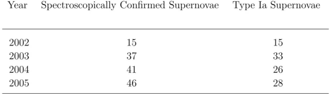
(20) – 20 – Weather and observing conditions for 2003 were greatly improved over 2002, though still somewhat sub-standard for typical conditions at Cerro Tololo. Unfortunately, one of the MOSAIC CCDs (containing amplifiers 5 and 6) failed shortly before the observations began, resulting in a 12.5% loss in efficiency. The failed CCD was replaced before our 2004 observing season, allowing us to recover the lost efficiency from then on. For the third year and fourth years of ESSENCE, we maintained the same set of fields as in 2003 and the MOSAIC imager was stable. The supernovae yields for each of the four years of the survey are summarized in Table 2. The ESSENCE search is successful and our program finds roughly twice as many objects with SN-like light curves than we can follow up spectroscopically each year. Table 2. Summary of the supernova yields from the first four years of ESSENCE observations. Year. Spectroscopically Confirmed Supernovae. Type Ia Supernovae. 2002 2003 2004 2005. 15 37 41 46. 15 33 26 28.

(21) – 21 – 2.2.. Image Analysis Pipeline. The ESSENCE program requires immediate reduction of each night’s data (typically ∼ 4 GB each night), so it is more convenient to base operations at the NOAO/CTIO offices in the nearby city of La Serena, rather than directly at the telescope. Therefore, ESSENCE team members carry out observations remotely from a terminal at La Serena, communicating with telescope operators on the mountain via a video-conferencing link. Incoming data may be viewed by connecting directly to computers at the telescope, which allows real-time quality control, while in parallel the data are immediately transferred to computing hardware in La Serena via an internet link. The analysis of ground-based imaging data is a complicated multi-stage procedure, involving the removal of instrumental artifacts, calibration of the data and measurements of the fluxes from the objects of interest. The particular demands of a supernova survey place more demanding constraints on the image analysis software. First, the objects of interest are transient and appear in the data masked by the background flux from their host galaxy. Past experience has shown that the most reliable way to find these objects is via image subtraction (Norgaard-Nielsen et al. 1989; Perlmutter et al. 1995; Schmidt et al. 1998). For each new image, an archival “template” frame from a previous epoch is subtracted pixel-by-pixel to remove constant sources, such as galaxies, to reveal the supernovae. Image subtraction software is not part of standard analysis packages and we have invested significant effort in developing robust and reliable methods necessary for our project. Second, supernovae must be detected in real time. While it is a part of our search strategy to revisit each field and build up a time series of photometric measurements of all objects, we rely on follow-up spectroscopic observations to verify the identity of candidate transients as type Ia supernovae and to establish their redshifts. Because supernovae at the distances that give cosmological leverage are faint (m ∼ 22) even at maximum light, it is preferable to observe them near maximum light. Type Ia supernovae rise to maximum light roughly 20 days after explosion in their rest frame (Riess et al. 1999a; Conley et al. 2006; Garg et al. 2006), and while time dilation stretches the rise of a supernova by a factor of 1 + z, a prompt detection allows us to schedule the spectroscopic observations into the available time. This real-time component adds a significant demand on the analysis of the survey data: the data must be processed automatically and reliably, in bulk, each night of the survey. Finally, supernovae are rare events. We expect roughly one supernova per MOSAIC field per month. Each MOSAIC field consists of 4096 × 2048 × 8 = 67, 000, 000 pixels, and.

(22) – 22 – we must be able to reliably determine the ∼dozen pixels among those that contain signal, often only marginally above background noise, from a bona fide type Ia supernova. 2 We have developed a data pipeline that meets these demands, accepting raw images directly from the telescope and automatically producing lists of candidate objects only hours later. Floating point operations are carried out by a variety of programs, either drawn from publicly available astronomical software packages, such as IRAF3 , or written by us (generally in C). These are tied together by a suite of Perl scripts, which handle process management and bookkeeping. Functionally, there are two separate piplines. The first of these (“mscpipe”) performs tasks relevant for full MOSAIC images and as output divides each single MOSAIC field into sixteen 1k x 4k pixel images corresponding to each CCD amplifier. From this point onward, the “amplifier-images” are processed through “photpipe” and each amplifier is effectively treated as an independent detector. We will refer to a single MOSAIC exposure as a MOSAIC field and the subdivided images as subfields. Below we provide a brief description of the data processing, focusing in particular on those stages that alter the data in ways significant for the analysis.. 2.2.1. Crosstalk correction Pairs of CCDs in the MOSAIC II imager are read out through single electronics controllers, which, for some combinations of CCDs, results in low-level cross-talk between the signals from different chips. The resulting effect is the appearance of “ghosts” in one subfield of bright objects appearing in another subfield. Fortunately, this effect is small in magnitude, on the order of 0.1%, and deterministic. The first stage of the mscpipe pipeline uses the most recent values of these cross-talk coefficients measured by the observatory staff and subtracts these electronic artifacts from the affected portions of the MOSAIC field, using the xtalk task from the mscred package for IRAF. 2. If there are roughly 10 needles to a gram and a typical haystack weighs 1000 kilograms, then finding the part per 107 supernova pixels in one frame is truly like finding a needle in a haystack. And we need to sift 20 per night! 3. IRAF is distributed by the National Optical Astronomy Observatory, which is operated by AURA under cooperative agreement with the NSF..

(23) – 23 – 2.2.2. Astrometric calibration The transformation from pixel to sky coordinates is dominated by distortions due to the optical system of the telescope that change only slightly over long periods of time and generally take the form of a polynomial in radius. Once the terms of this distortion function are known, the astrometric calibration of any particular image reduces to determining accurately the center of the distortion in that field, essentially an offset in x and y and a rotation. This is accomplished via the IRAF task msccmatch from the mscred package, which matches objects in the image to an existing catalog of the field with precise astrometry. The current standard for astrometry is the USNO CCD Astrograph Catalog 2 (UCAC, Zacharias et al. (2004)) , which covers all fields observed by ESSENCE. However, since ESSENCE is a significantly deeper survey, the Sloan Digital Sky Survey (SDSS, York et al. (2000)) provides a better photometric overlap. We use the SDSS (which itself is tied to UCAC) in the fields for which SDSS has imaging data (∼ 73% of ESSENCE fields), and default to UCAC when there is no SDSS data. When the supernovae are faint, their location in an image is poorly constrained, and we must rely on the astrometric solution to tell us precisely where to measure the flux. Errors in positioning the PSF produce an underestimate the object’s flux. Therefore, accurate relative astrometric calibration is essential to measuring supernova flux at low signal-to-noise, since what matters is that we are able to map pixels from invididual images to some consistent coordinate system. To this end, we generate astrometric catalogs from our own data, which are themselves calibrated to either SDSS or UCAC. All subsequent ESSENCE images are then registered to these internally generated catalogs. The astrometric solution is also used to “warp” each image to a common pixel coordinate system, so that reference images can be subtracted from them. This is accomplished using the SWarp (Bertin et al. 2002) software package, using a Lanczos windowed sinc function to resample the pixels onto the new coordinate system.. 2.2.3. Flatfielding In order to obtain consistent flux measurements across the plane of MOSAIC imager, we must normalize the response of all the pixels. This flat fielding is achieved in three steps. First, at the beginning of each night, a screen inside the telescope dome is illuminated and observed with the MOSAIC. These high signal-to-noise flatfields enable us to accurately correct for pixel-to-pixel variations and other imperfections in the optical system, but introduces large-scale variations (e.g. gradients due to non-uniform illumination of the flat-field screen)..

(24) – 24 – The second step is to combine all of the data from a night’s observations. By masking all astronomical sources and combining with a median statistic, an image of the illumination of the focal plane due to the night sky is created. This “illumination correction” is also applied to the data, removing gradients of ∼ 1% across a CCD. Finally, we use the average difference in sky level between each ccd to further regularize the overall flux scaling, a 1% correction to the dome flats.. 2.2.4. Photometric calibration Flat-fielded and SWarped images are then analyzed with the DoPHOT photometry package (Schechter et al. 1993) to identify and measure sources. This instrumental photometry is then calibrated against a catalog of objects with known magnitudes, to determine the photometric zeropoint for the image. Further discussion of photometric calibrations follows in Section 3.. 2.2.5. Image subtraction Each image is then differenced against a reference image. This suppresses all constant sources of flux and reveals transients such as new supernovae. To subtract two images taken under different atmospheric conditions on different nights, we must correct for seeing variations. Our image subtraction software uses the algorithm devised by Alard and Lupton (Alard & Lupton 1998; Alard 2000) to determine and apply a convolution that matches the point-spread functions of the two images prior to subtraction. Improvements to the basic method have produced a process that automatically, robustly, and reliably produces clean subtractions in our data.. 2.2.6. Difference image object detection Object detection in the subtracted images is done with a modified version of DOPHOT. Resampling and convolution of the images correlates flux between pixels, so we have modified the image registration and subtraction software to propagate noise maps that track these correlations. These are then used to evaluate the significance of objects detected in the difference image..

(25) – 25 – 2.3.. Candidate selection. Each observation of a single ESSENCE field yields hundreds of objects detected above some significance threshold in the subtracted images. These must be culled to produce a small set of objects that are very likely to be type Ia supernovae and merit spectroscopic observation on large telescopes. We first apply a series of software cuts, which include • requiring that the object has the same PSF as stars in the original, unsubtracted image, • vetoing detections with significant amounts of pixels with negative flux, to guard against subtraction residuals, such as dipoles resulting from slight image misalignment, • vetoing variable sources identified in previous data (variable stars, active galactic nuclei) and • requiring coincident detections in more than one passband or on subsequent nights, to reject asteroids (typically, two detections at signal-to-noise ratio > 5 within a five day window). While the above rules eliminate many of the false positives, we ultimately rely on human inspection to reject the small fraction of contaminants that evade these filters. Common problems include insufficient masking of pixels from bright stars, subtraction artifacts, and variable objects that have not varied significantly in previous ESSENCE data. We also perform light curve fits to assess whether each object is consistent with the known behavior of SN Ia. Preliminary fits of the initial R and I photometry are compared with light curve templates of a type Ia SN at z=0 in B and V filters (which are a good match for SN Ia at z∼0.4-0.5). The template light curve is representative of a normal type Ia SN with ∆m15 = 1.1 mag, or stretch=1, and was contructed from well-sampled light curves of low-z supernovae (Prieto et al. 2006). Using a chi-squared minimization, we determine the the best fit values for time of B maximum, observed R and I magnitudes at maximum, and stretch. We chose to use stretch here because it parametrizes in a simple way the variety of light curve shapes of SNe Ia (Goldhaber et al. 2001). Using the R and I magnitudes at maximum and the stretch obtained from the fit, we can now estimate a photometric redshift assuming that the candidate is a type Ia SN. A standard ΛCDM with ΩM = 0.3, ΩΛ = 0.7 is used and no host galaxy reddening is considered in these fits. A summary of the data for each candidate object is presented on a web page for human inspection. We reject detections resulting from subtraction artifacts by looking at image “stamps” at the position of the supernova. The light curves from the preliminary photometry.

(26) – 26 – enable us to reject objects that clearly have the wrong light curve shape, color, and brightness for a supernova in the estimated redshift range. Because our spectroscopy resources are limited, we have to make choices to observe the most promising targets. We select against objects right at the centers of galaxies both because past experience has shown that these are frequently active galactic nuclei and because contamination from the galaxy often makes it impossible to positively identify the supernova in a spectrum. To avoid these problems, we select against candidates that are superposed on point-like sources in the central pixel (0.27”) of the template image. We know that the SN Ia in galaxy centers have a broader distribution in apparent luminosity from SN Ia generally (Jha et al. 2007), but we do not expect any significant cosmological bias from this selection criterion. The objects that pass the above selection procedure are then sent to team members for spectroscopic observation. Because spectroscopy time is limited and scheduled in advance, we are forced to prioritize those objects that look most promising based on the data available at the time. Our survey is spectroscopy-limited: at the end of each observing campaign, many objects remain that have Ia-like light curves, but for which we were unable to obtain follow-up spectroscopy. Nevertheless, we successfully detect and confirm new supernovae at a rate of roughly one new object per night of 4m observing..

(27) – 27 – 3. 3.1.. Spectroscopy Observations. Follow-up spectroscopic observations of ESSENCE targets are performed at a wide variety of ground-based telescopes: the 10-m Keck I (+LRIS; Oke et al. 1995) and II (+ESI, Sheinis et al. 2002; +DEIMOS, Faber et al. 2003) telescopes; the 8-m VLT (+FORS1; Appenzeller et al. 1998), Gemini North and South (+GMOS; Hook et al. 2003) telescopes; the 6.5-m Magellan Baade (+IMACS; Dressler 2004) and Clay (+LDSS2; Mulchaey 2001), MMT (+BlueChannel; Schmidt et al. 1989) telescopes. One target (d100.waa7 16; see Matheson et al. 2005) was confirmed as a Type Ia supernova using the FAST spectrograph (Fabricant et al. 1998) on the 1.5-m Tillinghast telescope at the F. L. Whipple Observatory (FLWO). The useful sample of supernovae from the ESSENCE program is limited by our ability to identify SNe Ia spectroscopically. Standard CCD processing and spectrum extraction are done with standard IRAF routines. Except for the VLT data, all the spectra are extracted using the optimal algorithm of Horne (1986). For the VLT data, we apply a novel extraction method based on twochannel Richardson-Lucy restoration (Blondin et al. 2005) to minimize contamination of the supernova spectrum by underlying galaxy light. The spectra are wavelength calibrated using calibration-lamp spectra (usually HeNeAr). For the flux calibration we use both standard IRAF routines and our own IDL procedures, which include the removal of telluric lines using the well-exposed continua of the spectrophotometric standard stars (Wade & Horne 1988; Matheson et al. 2000b).. 3.2.. Supernova classification and redshift determination. Supernovae are classified according to their early-time spectra (see Filippenko 1997, for a review). The distinctive spectroscopic signature of a Type Ia supernova near maximum light is a deep absorption feature due to Si ii λ6355, blueshifted by ∼ 10000 km s−1 . Their spectra are further characterized by the absence of hydrogen and helium lines, although hydrogen has been detected in the spectrum of the Type Ia supernova SN 2002ic (Hamuy et al. 2003; Wood-Vasey et al. 2004) (Benetti et al. (2006) classify this object as an Type Ib/c). Spectra of Type Ib supernovae are characterized by a weaker Si ii λ6355 absorption, and by the presence of lines of He I. Spectra of Type Ic supernovae are devoid of He I lines and display only a weak Si ii λ6355 absorption. Thus, in principle, SNe Ib/c are readily distinguishable from SNe Ia..

(28) – 28 – At high (z & 0.4) redshifts, however, the defining Si ii λ6355 feature in SNe Ia is redshifted out of the optical range of most of the spectrographs we use, so features blueward of this must be used to establish the type. The most prominent of these, the Ca ii H&K λλ3934,3968 doublet, is also present in SNe Ib/c and does not discriminate between the various supernova types. Instead, the identification of SNe Ia relies on weaker features (e.g., Si ii λ4130, Mg ii λ4481, Fe ii λ4555, Si iii λ4560, S ii λ4816, and Si ii λ5051). While the above gives the general defining features of Ia spectra, in practice, identfying SNe Ia can be difficult in low signal-to-noise spectra, particular when trying to discriminate between SNe Ia and SNe Ib/c. In addition, we would like to establish objective and reproducible criteria for classifying objects, rather than relying on subjective assessments of noisy data. Therefore, we have developed an algorithm (SuperNova IDentification, or SNID; Blondin & Tonry 2007) also used by Matheson et al. (2005), which we use here to establish our final SN Ia sample. This algorithm cross-correlates an input spectrum with a library of supernova spectra, without attempting to directly identify specific features, and a redshift is determined based on the shift in wavelength that maximizes the correlation. The spectral database currently spans all supernova types and covers a wide range of ages, containing 796 spectra of 64 SNe Ia (including spectra of 1991T-like and 1991bg-like objects), 288 spectra of 17 SNe Ib/c, and 353 spectra of 10 SNe II. We also include spectra of galaxies, AGNs, and stars to identify spectra that are not consistent with a supernova (see also Matheson et al. 2005). The results of the SNID analysis are shown in Table 3. The correlation redshift is valid when templates of the correct supernova type are used. We also use SNID to determine the supernova type, by computing the absolute fraction of “good” correlations that correspond to supernovae of different types. The supernova types/subtypes in the SNID spectral database are: Ia/Ia-norm, Ia-pec, Ia-91t, Ia-91bg; Ib/Ib-norm, Ib-pec, IIb; Ic/Ic-norm, Ic-pec, Ic-broad; II/II-norm, II-pec, IIL, IIn, IIP, IIb. “Norm” and “pec” subtypes are used to identify the spectroscopically “normal” and “peculiar” supernovae of a given type, respectively. For type Ia supernovae, “91t” and “91bg” indicates spectra that resemble those of the overluminous SN 1991T and the underluminous SN 1991bg, respectively. The spectra that correspond to the “Ia-pec” category in this case are those of SNe 2000cx (Li et al. 2001a; Candia et al. 2003) and 2002cx (Li et al. 2003). For type Ic supernovae, ‘Ic-broad” is used to identify broad-lined SNe Ic, (often referred to as “hypernovae” in the literature), some of which are associated with Gamma-Ray Bursts. The notation used for the type II subtypes are commonly used in the literature. Note that type IIb supernovae (whose spectra evolve from a type II to a type Ib, as, e.g., in SN 1993J– see Matheson et al. 2000a) are included both in the “Ib” and “II” types. If the redshift of the supernova host galaxy can be measured using narrow emission or.

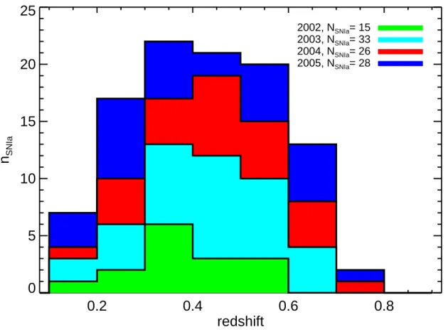
(29) – 29 – absorption lines, we force SNID to look for correlations at the galaxy redshift (±0.03) to determine the supernova type/subtype; otherwise the redshift is left as a free parameter. We assert a supernova to be of a given type (i.e., Ia, Ib, Ic, II, see Table 3, column 3) when the absolute fraction of “good” correlations that correspond to this type exceeds 50%. In addition, we require the best-match supernova template to be of the same type. We determine the supernova subtype by requiring that the absolute fraction of “good” correlations that correspond to this subtype exceeds 50%, and that it corresponds to the previouslydetermined type. We also require that the best-match supernova template is of the same subtype. The requirement that an object must have a correlation fraction above 50% is motivated by the desire to have a quantative figure of merit that determines when the spectral information is strong enough to make a positive identification. Out of all the spectra that were considered to be those of possible supernovae, 28 did not meet the above criteria for a positive classification (see Table 3). Assessing the likelihood that a spectrum matches that of particular known object more closely than others is a challenging statistical problem, especially in the presence of intrinsic and only partially understood variance in the populations of supernovae. See Blondin & Tonry (2007) for a detailed discussion of ongoing work to better understand these issues. The redshift is then determined from the supernova spectrum alone in a second SNID run by considering correlations with templates of the determined type and subtype. No a priori information on redshift is used in this second run. The supernova redshift is reported as the median redshift of all “good” correlations, and the redshift error as the standard deviation of these same redshifts. When there is only one “good” correlation for an input spectrum (objects d087, h311, and p524 in Table 3), we quote the redshift as that of the best-match template and the associated error as the formal redshift error for that template (see Blondin & Tonry 2007). We only report a SN redshift when a secure type is determined. In Matheson et al. (2005) we found an excellent agreement between the SNID correlation redshift and the redshift of the supernova host galaxy when it is known from other methods. Figure 4 again shows that the SNID redshifts agree well with the galaxy redshifts, with a typical uncertainty . 0.01 in the redshift range [0.1 − 0.8]. Figure 5 shows the redshift distribution of the spectroscopically confirmed SNe Ia from the first four years of ESSENCE..

(30) Table 3. Types and Redshifts of ESSENCE Supernovae. RA [J2000]. Dec [J2000]. ESSENCE ID. 2002iu 2002iv 2002jq 2002iy 2002iz 2002ja 2002jb 2002jr 2002jc 2002js 2002jd 2002jt 2002ju 2002jw — 2003jo 2003jj 2003jn 2003jm 2003jv 2003ju 2003jr 2003jl 2003js 2003jt 2003ji 2003jq 2003jw 2003jy 2003kk 2003kl 2003km 2003kn 2003ko. 00:13:33.10 02:19:16.11 23:35:57.96 02:30:40.00 02:31:20.73 23:30:09.66 23:29:44.14 02:04:41.03 02:07:27.28 02:20:35.39 00:28:38.39 00:13:36.70 02:20:11.00 02:30:00.52 00:28:03.16 23:25:24.03 01:07:58.52 02:29:21.21 02:28:50.93 23:27:58.22 23:27:01.71 01:11:06.23 02:28:28.56 02:29:52.15 02:31:54.60 02:07:54.84 23:30:51.19 02:31:06.84 02:10:53.98 23:25:36.06 01:09:48.80 02:30:01.00 02:09:15.55 02:11:06.48. -10:13:09.92 -07:44:06.72 -10:05:56.88 -08:11:40.50 -08:36:13.12 -09:35:01.75 -09:36:34.25 -05:09:40.73 -03:50:20.73 -09:34:43.90 +00:40:29.29 -10:08:24.00 -09:04:37.50 -08:36:22.41 +00:37:50.43 -09:26:00.63 +00:03:01.89 -09:02:15.57 -09:09:58.14 -08:57:11.82 -09:24:04.49 +00:13:44.21 -08:08:44.74 -08:32:28.09 -08:35:48.43 -03:28:28.40 -09:28:33.95 -08:45:36.51 -04:25:49.76 -09:31:44.70 +01:00:05.58 -09:04:35.89 -03:35:41.38 -03:47:56.09. b003 b004 b008 b010 b013 b016 b017 b020 b022 b023 b027 c003 c012 c015 c023 d033 d058 d083 d084 d085 d086 d087 d089 d093 d097 d099 d100 d117 d149 e020 e029 e108 e132 e136. Type. Subtype. Ia Ia Ia Ia Ia Ia Ia Ia Ia Ia Ia Ia Ia Ia Ia Ia Ia Ia Ia Ia Ia Ia Ia Ia Ia Ia Ia Ia Ia Ia Ia Ia Ia Ia. Ia-norm Ia-91t Ia-norm Ia-norm Ia-norm Ia-norm Ia-norm Ia-norm Ia-norm Ia-norm Ia-norm —a Ia-norm Ia-norm Ia-norm Ia-norm Ia-norm Ia-91t Ia-norm Ia-91t Ia-norm Ia-norm Ia-norm Ia-91t Ia-norm Ia-norm Ia-norm Ia-norm Ia-norm Ia-norm Ia-norm Ia-norm Ia-norm Ia-norm. %Subtype. 74.2 64.4 65.1 73.6 85.8 100.0 75.5 81.8 55.7 90.9 79.2 — 72.6 76.6 100.0 76.0 85.0 56.5 68.6 100.0 87.5 100.0 92.3 63.1 95.7 77.5 67.8 84.6 100.0 88.4 74.7 100.0 76.3 85.1. %Ia. 100.0 98.3 81.4 82.4 98.6 100.0 100.0 100.0 65.7 100.0 96.6 100.0 100.0 100.0 100.0 96.0 95.0 100.0 100.0 100.0 100.0 100.0 100.0 93.4 100.0 96.9 98.3 100.0 100.0 100.0 100.0 100.0 100.0 99.2. %Ib/c. 0.0 1.7 11.6 17.6 1.4 0.0 0.0 0.0 24.3 0.0 3.4 0.0 0.0 0.0 0.0 4.0 5.0 0.0 0.0 0.0 0.0 0.0 0.0 6.6 0.0 2.0 1.7 0.0 0.0 0.0 0.0 0.0 0.0 0.8. %II. zGAL. zSNID. σz. 0.0 0.0 7.0 0.0 0.0 0.0 0.0 0.0 10.0 0.0 0.0 0.0 0.0 0.0 0.0 0.0 0.0 0.0 0.0 0.0 0.0 0.0 0.0 0.0 0.0 1.0 0.0 0.0 0.0 0.0 0.0 0.0 0.0 0.0. — 0.231 — 0.587 0.428 — — — — — — — 0.348 0.357 0.399 0.524 0.583 — 0.522 0.405 — 0.340 0.429 0.363 — — — 0.296 0.339 0.164 0.335 — 0.244 0.360. 0.115 0.226 0.474 0.590 0.426 0.329 0.258 0.425 0.540 0.550 0.318 0.382 0.350 0.362 0.400 0.531 0.583 0.333 0.519 0.401 0.205 0.337b 0.436 0.360 0.436 0.211 0.156 0.309 0.342 0.159 0.332 0.469 0.239 0.352. 0.006 0.003 0.004 0.006 0.004 0.003 0.007 0.003 0.008 0.007 0.005 0.002 0.006 0.008 0.009 0.008 0.009 0.002 0.007 0.001 0.003 0.009 0.006 0.004 0.008 0.003 0.003 0.006 0.006 0.007 0.008 0.005 0.006 0.007. – 30 –. IAUC ID.

(31) Table 3—Continued RA [J2000]. Dec [J2000]. ESSENCE ID. 2003kt 2003kq 2003kp 2003kr 2003ks 2003kuc 2003kvc 2003lh 2003le 2003lf 2003lm 2003ll 2003lkd 2003ln 2003lj 2003li —d — 2004fic 2004fh 2004fj 2004fn 2004fm 2004flc 2004fk — 2004fo — — 2004fqc 2004fs 2004frc 2004ftc —c. 02:33:47.01 02:31:04.09 02:31:02.64 02:31:20.96 02:31:34.54 01:08:36.25 02:09:42.52 02:10:19.51 01:08:08.73 01:08:49.81 23:24:25.51 02:35:41.19 02:11:12.82 23:30:27.15 01:12:10.03 02:27:47.29 02:27:26.51 02:29:22.39 23:29:45.35 23:28:27.20 01:09:51.07 23:30:20.12 23:26:58.14 23:26:57.92 01:13:35.84 23:27:37.16 01:13:28.97 02:09:49.63 23:28:37.70 23:27:45.64 02:31:19.95 02:28:43.77 02:33:32.63 23:27:15.69. -08:36:22.09 -08:10:56.64 -08:39:50.81 -08:36:14.16 -08:36:46.41 -00:33:20.78 -03:46:48.58 -04:59:32.30 +00:27:09.74 -00:44:13.49 -08:45:51.11 -08:06:29.55 -04:13:52.11 -08:35:46.98 +00:19:51.29 -07:33:46.16 -08:42:24.88 -08:37:38.38 -08:54:36.34 -08:36:55.17 +00:27:20.95 -09:58:30.67 -09:37:19.45 -09:37:19.11 -00:09:27.56 -09:35:20.96 +00:35:16.26 -04:10:55.07 -08:45:04.01 -08:31:12.77 -08:49:21.67 -08:54:24.05 -08:09:34.10 -09:27:59.76. e138 e140 e147 e148 e149 e315 e531 f011 f041 f076 f096 f216 f221 f231 f235 f244 f301 f308 g001 g005 g043 g050 g052 g053 g055 g097 g120 g133 g142 g151 g160 g166 g199 g225. Type. Subtype. Ia Ia Ia Ia Ia — — Ia Ia Ia Ia Ia — Ia Ia Ia — Ia — Ia II Ia Ia — Ia Ia Ia Ia Ia — Ia — — —. Ia-norm Ia-norm Ia-norm Ia-norm Ia-norm — — Ia-norm Ia-norm Ia-norm Ia-norm Ia-norm — Ia-norm Ia-norm Ia-norm — Ia-norm — Ia-norm IIP Ia-norm Ia-norm — Ia-norm Ia-norm Ia-norm Ia-norm Ia-norm — Ia-norm — — —. %Subtype. 100.0 100.0 100.0 100.0 81.4 — — 100.0 68.8 82.2 88.5 75.0 — 100.0 87.8 100.0 50.0 66.7 — 72.9 100.0 100.0 80.0 — 79.3 62.8 94.7 75.0 58.2 — 89.5 — — —. %Ia. 100.0 100.0 100.0 100.0 98.6 — — 100.0 100.0 100.0 100.0 100.0 33.3 100.0 100.0 100.0 75.0 100.0 — 100.0 0.0 100.0 100.0 — 100.0 81.4 100.0 98.8 98.5 — 100.0 — — —. %Ib/c. 0.0 0.0 0.0 0.0 1.4 — — 0.0 0.0 0.0 0.0 0.0 66.7 0.0 0.0 0.0 14.3 0.0 — 0.0 0.0 0.0 0.0 — 0.0 18.6 0.0 0.0 1.5 — 0.0 — — —. %II. zGAL. zSNID. σz. 0.0 0.0 0.0 0.0 0.0 — — 0.0 0.0 0.0 0.0 0.0 0.0 0.0 0.0 0.0 10.7 0.0 — 0.0 100.0 0.0 0.0 — 0.0 0.0 0.0 1.2 0.0 — 0.0 — — —. — 0.606 — 0.427 — — — — — — 0.408 0.596 0.442 — 0.417 0.544 — — 0.265 — 0.187 0.605 — — 0.296 0.343 — — 0.404 0.146 — 0.202 — —. 0.612 0.631 0.645 0.429 0.497 — — 0.539 0.561 0.410 0.412 0.599 — 0.619 0.422 0.540 — 0.394 — 0.218 0.193 0.633 0.383 — 0.302 0.340 0.510 0.421 0.399 — 0.493 — — —. 0.009 0.007 0.010 0.006 0.006 — — 0.004 0.006 0.007 0.006 0.005 — 0.008 0.007 0.004 — 0.009 — 0.007 0.002 0.006 0.008 — 0.006 0.004 0.009 0.003 0.003 — 0.003 — — —. – 31 –. IAUC ID.

(32) Table 3—Continued RA [J2000]. Dec [J2000]. ESSENCE ID. —d — —c 2004ha — 2004hc 2004hd 2004he 2004hf 2004hgc 2004hi 2004hh 2004hj 2004hkc — 2004hl 2004hm 2004hn —c 2004hq 2004hpc 2004hr —c 2004hs —c —c — —c — — — — — —. 01:11:56.31 23:30:41.83 02:04:27.01 02:04:27.01 02:31:40.67 23:24:32.67 02:08:48.21 02:29:48.79 02:32:00.14 02:34:55.19 02:08:38.84 02:06:25.02 02:29:41.94 23:27:04.39 23:26:11.77 01:13:38.17 02:28:03.12 01:13:32.39 01:13:38.17 02:30:18.04 02:09:35.52 01:08:48.34 02:31:11.80 02:09:33.69 02:30:24.32 01:08:22.01 02:05:27.31 02:30:27.27 02:31:46.24 02:08:06.23 02:07:12.91 23:30:02.70 23:28:39.97 01:09:15.01. +00:07:27.71 -08:34:10.98 -03:35:43.72 -04:52:46.03 -08:49:03.35 -08:41:03.55 -04:26:10.42 -08:20:45.94 -08:42:23.89 -08:30:43.64 -05:08:11.79 -04:38:04.09 -08:43:49.42 -08:38:45.11 -08:50:17.50 -00:27:39.03 -07:42:29.70 +00:37:15.38 -00:27:39.03 -08:22:25.01 -03:46:23.53 +00:00:49.49 -07:47:34.13 -04:13:03.93 -07:53:20.95 -00:05:46.65 -04:42:54.05 -09:16:10.23 -09:16:25.65 -04:03:51.16 -04:26:40.06 -08:33:36.57 -09:19:50.00 +00:08:14.80. g230 g240 g276 h283 h300 h311 h319 h323 h342 h345 h359 h363 h364 k396 k411 k425 k429 k430 k432 k441 k443 k448 k467 k485 k490 m001 m003 m006 m010 m011 m014 m022 m026 m027. Type. Subtype. — Ia — Ia Ia Ia Ia Ia Ia — Ia Ia Ia — Ia Ia Ia Ia — Ia — Ia — Ia — — II — Ib II II Ia Ia Ia. — Ia-norm — Ia-norm Ia-norm Ia-norm Ia-norm Ia-norm Ia-norm — Ia-norm Ia-norm Ia-norm — Ia-norm Ia-norm Ia-norm Ia-norm — Ia-norm — Ia-norm — Ia-norm — — —a — Ib-norm IIP IIP —a —a Ia-norm. %Subtype. — 86.7 — 85.7 100.0 100.0 100.0 100.0 100.0 — 46.8 69.0 100.0 — 78.6 82.9 66.7 100.0 — 81.0 — 100.0 — 93.3 — — 34.2 — 100.0 78.1 50.0 — — 72.2. %Ia. 50.0 100.0 — 100.0 100.0 100.0 100.0 100.0 100.0 — 68.1 97.7 100.0 — 85.7 97.1 100.0 100.0 — 100.0 — 100.0 — 100.0 — — 2.6 — 0.0 0.0 0.0 93.8 97.8 92.6. %Ib/c. 0.0 0.0 — 0.0 0.0 0.0 0.0 0.0 0.0 — 31.9 0.0 0.0 — 14.3 0.0 0.0 0.0 — 0.0 — 0.0 — 0.0 — — 0.0 — 100.0 0.0 0.0 1.8 2.2 7.4. %II. zGAL. zSNID. σz. 50.0 0.0 — 0.0 0.0 0.0 0.0 0.0 0.0 — 0.0 2.3 0.0 — 0.0 2.9 0.0 0.0 — 0.0 — 0.0 — 0.0 — — 97.4 — 0.0 100.0 100.0 4.4 0.0 0.0. 0.392 — 0.244 — — — 0.490 0.598 — — — — — — — 0.270 0.172 — — — — 0.409 — — 0.715 — — 0.057 0.216 0.205 0.200 — 0.655 0.289. — 0.687 — 0.502 0.687 0.741b 0.495 0.603 0.421 — 0.348 0.213 0.344 — 0.564 0.274 0.181 0.582 — 0.680 — 0.401 — 0.416 — — 0.219 — 0.222 0.211 0.212 0.240 0.653 0.286. — 0.005 — 0.008 0.012 0.011 0.004 0.006 0.002 — 0.004 0.006 0.007 — 0.006 0.003 0.008 0.010 — 0.010 — 0.005 — 0.005 — — 0.001 — 0.001 0.002 0.003 0.003 0.008 0.006. – 32 –. IAUC ID.

(33) Table 3—Continued RA [J2000]. Dec [J2000]. ESSENCE ID. — — — — — — — — — — — — — — — — — — — — — — — — — — — — — — — — — —. 23:29:35.34 02:27:50.33 02:05:10.83 02:28:04.63 02:09:49.78 23:29:51.73 02:10:56.77 01:09:52.90 23:24:42.28 01:08:56.35 23:23:57.83 23:24:03.53 02:28:52.20 02:06:03.69 01:14:33.08 02:28:09.01 02:06:42.35 02:05:14.95 01:13:06.51 23:28:17.55 23:23:51.35 02:29:00.48 23:29:58.59 23:30:32.01 01:13:13.26 02:31:31.43 02:31:19.60 23:29:56.19 01:12:40.25 02:08:32.45 02:11:00.02 02:08:09.34 02:30:10.16 02:08:10.47. -09:58:46.33 -07:59:11.62 -04:47:13.94 -07:42:44.29 -04:45:10.65 -08:56:46.07 -04:27:29.90 +00:36:19.03 -08:29:07.82 +00:39:25.38 -08:27:08.33 -09:23:18.24 -07:42:09.78 -04:39:59.12 -00:26:23.18 -07:47:49.56 -04:22:37.01 -04:56:39.08 +00:30:04.86 -09:23:12.38 -08:23:18.47 -09:02:52.96 -08:53:12.45 -10:03:22.14 -00:23:25.86 -08:55:11.52 -08:45:09.76 -08:34:24.34 +00:14:56.61 -03:33:34.20 -04:09:37.59 -03:48:05.05 -08:52:50.84 -03:32:17.70. m032 m034 m038 m039 m041 m043 m057 m062 m075 m138 m139 m158 m193 m226 n246 n256 n258 n263 n271 n278 n285 n322 n326 n368 n400 n404 n406 p425 p434 p454 p455 p520 p524 p527. c. c. c. c. c. c. c. Type. Subtype. Ia Ia II Ia II Ia Ia Ia Ia Ia II Ia Ia Ia — Ia Ia Ia II Ia Ia — Ia Ia — Ia — Ia — Ia Ia — Ia —. Ia-norm Ia-norm IIP Ia-norm —a Ia-norm —a —a —a Ia-norm —a —a Ia-norm —a — Ia-norm Ia-norm Ia-norm IIP Ia-norm Ia-norm — Ia-norm Ia-norm — Ia-norm — Ia-norm — Ia-norm Ia-norm — Ia-norm —. %Subtype. 80.2 96.3 94.4 84.4 — 57.3 — — — 66.7 — — 100.0 — — 100.0 50.0 79.9 85.2 78.5 64.5 — 79.8 83.1 — 100.0 — 100.0 — 100.0 88.9 — 100.0 —. %Ia. 96.5 100.0 5.6 100.0 22.8 99.5 95.5 100.0 100.0 100.0 0.0 95.2 100.0 95.2 — 100.0 81.6 100.0 0.0 100.0 81.4 — 100.0 100.0 — 100.0 — 100.0 61.7 100.0 100.0 — 100.0 —. %Ib/c. 3.5 0.0 0.0 0.0 0.0 0.0 0.4 0.0 0.0 0.0 0.0 4.8 0.0 4.8 — 0.0 18.4 0.0 0.0 0.0 14.5 — 0.0 0.0 — 0.0 — 0.0 33.3 0.0 0.0 — 0.0 —. %II. zGAL. zSNID. σz. 0.0 0.0 94.4 0.0 77.2 0.5 4.1 0.0 0.0 0.0 100.0 0.0 0.0 0.0 — 0.0 0.0 0.0 100.0 0.0 4.1 — 0.0 0.0 — 0.0 — 0.0 4.9 0.0 0.0 — 0.0 —. — 0.557 0.051 0.248 — 0.266 0.180 0.314 0.100 0.587 0.212 — 0.330 0.675 0.706 — — — — 0.304 — — 0.264 0.342 0.424 — — 0.458 0.339 — 0.298 — — 0.435. 0.155 0.562 0.054 0.249 0.220 0.266 0.184 0.317 0.102 0.582 — 0.463 0.341 0.671 — 0.631 0.522 0.368 0.241 0.309 0.528 — 0.268 0.344 — 0.216 — 0.453 — 0.695 0.284 — 0.508b —. 0.004 0.006 0.003 0.003 0.004 0.003 0.003 0.005 0.001 0.004 — 0.007 0.009 0.004 — 0.012 0.007 0.007 0.004 0.006 0.006 — 0.006 0.006 — 0.008 — 0.006 — 0.010 0.006 — 0.009 —. – 33 –. IAUC ID.

(34) – 34 – 4. 4.1.. Photometry of ESSENCE supernovae Importance of Photometric Calibration. Our ability to determine cosmological parameters from the observations of supernovae depends on measuring the fluxes of these objects accurately. Errors in photometric calibration translate into errors in the cosmology in two basic ways. First, we must understand the calibration of our supernovae fluxes to those of the low-redshift sample (Hamuy et al. 1993; Riess et al. 1999b; Jha et al. 2006). Light curve fitting and luminosity estimation methods have been trained using these objects and they also serve the “anchor” for the Hubble diagram in our cosmological measurements of the evolution of the scale factor. Second, accurate passband-to-passband calibration is important for estimating the colors of our supernovae, to provide constraints on extinction due to host galaxy dust. See the discussion in Wood-Vasey et al. (2007) for a discussion of how these calibration issues impact our cosmological measurements. Photometric systems are defined by the broadband fluxes of a single standard star (conventionally Vega, though more recently the Sloan Digital Sky Survey and others have used the F0 subdwarf BD+17◦ 4708), as well as a network of standard stars whose fluxes have been calibrated relative to the primary standard (Landolt 1983, 1992), and the wavelengthdependent sensitivities of that system. Observers usually account for the difference between the particular system they are using and the standard system by correcting their observations through terms proportional to the broad-band colors. These linear corrections can be quite accurate when derived from observations of standard stars and then applied to correct the photometry of other stars observed, since stellar spectra are generally relatively smooth. However, supernovae have complex spectra with broad and deep features, and they evolve in time, so the corrections derived from observations of stars are not appropriate for calibrating supernova fluxes into a standard system. To avoid additional error from converting the observed supernova fluxes to a ”standard” system, we report our photometry in the natural system of the CTIO 4m MOSAIC camera: m = −2.5 log F (ADU) + zeropoint,. (5). where the zeropoints are defined relative to the star Vega. It is important to note that in the process of defining a Vega-based standard star system, the “true” magnitudes of Vega have actually drifted and are slightly non-zero (Bessell et al. 1998; Bohlin & Gilliland 2004; Bohlin 2006). While these offsets amount to changes in the flux scale of only a few percent, they become significant for cosmological measurements at the level of precision we desire.