Model predictive control of hydrogen production by renewable energy

Texto completo

(1)PREPRINT. Model predictive control of hydrogen production by renewable energy Alvaro Serna. Julio E. Normey-Rico. Fernando Tadeo. Dept. de Ingeniería de Sistemas y Automática Universidad de Valladolid (UVA) Valladolid, Spain [email protected]. Dept. de Automação e Sistemas Universidade Federal de Santa Catarina (UFSC) Florianópolis, Brazil [email protected]. Dept. de Ingeniería de Sistemas y Automática Universidad de Valladolid (UVA) Valladolid, Spain [email protected]. Abstract— This paper presents the formulation of a control strategy based on model predictive control ideas to produce hydrogen from renewable energy in an offshore platform. Power generation based on wave and wind energy is considered as energy source which feeds a set of electrolyzers that produces hydrogen. The proposed advanced control system allows to regulate the operation of the electrolyzers, taking into account the renewable energy available and optimizing the performance of the plant. Simulation results obtained using a specific case study are presented, showing the correct operation of the plant under this advanced control. Keywords—hydrogen; renewable energy; predictive control; marine energies. I.. INTRODUCTION. This paper deals with a renewable energy offshore plant to produce hydrogen that was developed within the H2Ocean project [1]. The aim of this project was to study the technical feasibility of moving some technologies to an offshore location to reduce the demands on coastal resources and the associated environmental impact. In this context, the possibility of producing hydrogen directly in offshore wind and wave farms was evaluated. Hydrogen energy is considered one of the recent energy solutions that offer great advantages over many traditional energy sources [2]. The full benefits of hydrogen will be obtained when is produced from renewable energy sources [3]. Different renewable energy sources have already been studied for electrolyzation, such as wind [4,5], waves [6,7,8] and solar energy [9,10]; the feasibility of these sources to produce hydrogen has been demonstrated, with the main drawback their variability [10]. Hybrid refers to applications in which multiple energy conversion devices are connected together to produce the required energy. Such systems are often found in isolated applications and usually include renewable energy sources [11,12]. The sources considered in this work are wind and wave energy: wind energy is a technology that has matured to a level of development where it is ready to become generally accepted [13]. Wind power is playing an increasingly important role in electricity generation, especially in countries such as Germany or Spain [13]. In this project it is combined with wave energy because wave converters provide lower variability in the This work was funded by Ministerio de Ciencia e Innovación (Spain) under grant DPI2014-54530-R A. Serna and F. Tadeo are with the University of Valladolid, 47005 Valladolid, Spain (e-mail: [email protected]).. energy production in comparison with other sources [14]. Offshore power links are known to be significant expensive, so the system is here assumed to be fully isolated from the grid: it is parallel to the grid independent wind-hydrogen generation presented in [15]. Thus in our proposal, power consumption adapts to power production by connecting or disconnecting sections of the electrolyzation plant (following a Smart Grid approach for the microgrid in the plant) [3]. Compared with previous proposals [3,8], this paper concentrates on using an advanced control system to regulate the operation of the electrolyzers, taking into account the renewable energy available and optimizing the performance of the plant. In summary, the system used here is composed of two energy sources, namely wind and wave energy, which provide electricity in order to produce hydrogen using alkaline electrolyzers. An advanced control strategy is presented here, to connect/disconnect components, depending on the amount of energy available. The rest of the paper is organized as follows. Section II presents the studied problem and revises main properties of model predictive control. Section III presents the proposed control strategy and Section IV the simulated case study. The paper ends with a conclusion section. II.. PROBLEM STATEMENT. A. Description of components Fig. 1 presents the components of the electrolysis plant: Wind Energy. Demineralized Water (H2O). Wave Energy. Electricity. Hydrogen (H2). Electrolysis. Figure 1: General scheme of the electrolysis plant. Wind and waves are the energy sources, which are renewable, green and with a great capacity of research and development of their technologies. This energy is used in the electrolysis process that will be explained in the section below. If power supply changes with time, the production of hydrogen is going to change with time to adapt to the available power..

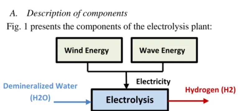
(2) PREPRINT Changing the working point of the plant by selecting a different operating point is proposed. B. Electrolysis Electrolyzation is a mature, market-available technique that can operate intermittently, producing large volumes of hydrogen, without greenhouse gases emissions, if electricity is provided by renewable sources. There exist a few promising electrolysis technologies [3]. These are polymer electrolysis (PEMEC), alkaline cells and solid oxide electrolysis (SOEC) [16]. PEMEC and alkaline based electrolysis are commercial technologies. The SOEC technology is a promising technology, although too immature. The investigated electrolyzer systems are all capable to generate hydrogen with a purity of > 99.97%, which is the quality used in the automotive industry [17]. Alkaline electrolyzers were chosen as it is the most developed and cheapest technology in offshore plants [18]. C. Model predictive control(MPC) MPC has gained popularity in industry since the 1990s and there is a steadily increasing attention from control practitioners and theoreticians [19]. The main advantage of MPC is the fact that today´s processes need to be operated under tight performance specifications and many constraints need to be satisfied [20]. The main elements in MPC are the objective function to be minimized, the model used to compute the predictions of the controlled variables, the definition of the process constraints and the method applied to solve the optimization problem. All these points are discussed in Section III for the case study. III.. CONTROL PROPOSAL. A. Control variables As it was mentioned in Section II, alkaline electrolyzers were selected to operate in the offshore platform. Two different types of alkaline electrolyzers are modelled in this paper: high production electrolyzers (nH is the number of devices of this type) and small production electrolyzers (being nS the number of this type). In order to design the control system of the plant, the following variables at each sample (k) are defined: 1) High production electrolyzers δi (k)ϵ {0,1}. . These binary variables correspond to each device being switched on or off. H and i subscripts are associated with these high production devices. 2) Small production electrolyzers 𝛾j (k)ϵ {0,1}. . These variables are equivalent to the ones in (1) (S and j are the associated subscripts). 3) Operating point for each electrolyzer H H αH  i (k) ϵ [ αi α i ] αSj (k) ϵ [ αSj α Sj ]. . Its minimum and maximum values are defined by α and α.. 4) Hydrogen production of each class of electrolyzers It is defined by the following variables below: HiH (k)    HjS (k) . . . 5) Power consumption for each class of electrolyzers: PiH (k)   PjS (k)   B. Modelling for control porposes The models for each class of electrolyzers are obtained from data sheet. Both are linear and depend on the operating point, that is a real number bounded by (3) and (4) and the on/off variables (which are binary). 1) High production electrolyzers H H PiH (k) = Pmax i ∙ αi (k)  HiH (k) = K H ∙ αH i (k) ∙ δi (k) where K H =. . . . . PH max i. . Performance(i). . Performance(i) = AH ∙ αH i (k) + BH. In these equations PiH is the power consumption of the H device at time k and Pmax i is the maximum power, while H H Hi is the production. AH, BH and Pmax i are empirical variables. 2) Small production electrolyzers S S PjS (k) = Pmax j ∙ αj (k). . HjS (k) = K S ∙ αSj (k) ∙ γj (k) where K S =.  . PS max j Performance(j). Performance(j) = AS ∙ αSj (k) + BS.  . S Where AS, BS and Pmax j are empirical variables.. C. Control algorithm The MPC used in this case study includes a quadratic cost function J which considers, in a horizon of Nh samples, the error between the produced hydrogen (HiH and HjS ) and its H S desired values (Hmax and Hmax ) and also the number of elecrolyzers in operation (δi and 𝛾j ). With this, the optimization problem solved each sample time aims to optimize hydrogen production (HiH and HjS ) and minimizes de consumption (PiH and PjS ). Taking into account model predictive control ideas, the available power (Pavailable ) is predicted over the prediction horizon using meteorological data. Then, the future predictions of the output (hydrogen.

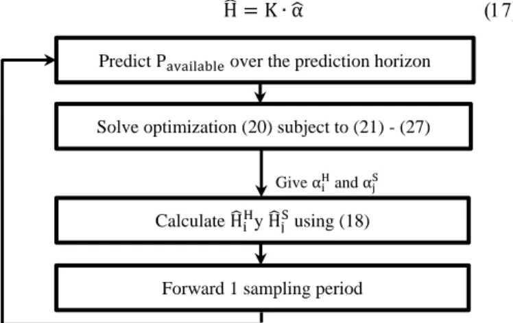
(3) PREPRINT ̂ ) are expressed as a function of the future production, vector H control actions (vector α ̂) and the past values of the input and outputs. In the case of the electrolyzers modelled in this paper, only a static model is considered, thus: ̂ =K∙α H ̂. . . . H αH i (k) − α i ∙ δi (k) ≤ 0. H H In this manner, the limits of αH i (k) are αi and α i when the electrolyzer is working, and are forced to be 0 when switched off. There is an analogy with the small production electrolyzers:. Predict Pavailable over the prediction horizon. αSj ∙ γi (k) − αSi (k) ≤ 0. . Solve optimization (20) subject to (21) - (27). αSj (k) − α Sj ∙ γj (k) ≤ 0. . Equation (20) is then transformed into the quadratic optimization described in (28):. S Give αH i and αj. ̂ iH y H ̂ jS using (18) Calculate H. 𝟏. 𝐉 = 𝐗 𝐓 ∙ 𝐇 ∙ 𝐗 + 𝐟 𝐓 ∙ 𝐗  𝟐. Figure 2: Control algorithm. Hydrogen produced for high production electrolyzers is: ̂H = K H ∙ α̂H H. . and for small production electrolyzers is: ̂S = K S ∙ α H ̂S. . T. H H ⃗ ) λH I(K H ∙ α̂H − Hmax ⃗) + 𝐉 =(K H ∙ α̂H − Hmax ∙1 ∙1 T. S S ⃗ ) λS I(K S ∙ α ⃗)+ (K S ∙ α ̂S − Hmax ∙1 ̂S − Hmax ∙1 T. T. . where λ𝑖 are the weight factors for the different parameters of the electrolyzers. The optimization problem solved each sample time has the following constraints: 1) Power consumed in each sample. This energy should be smaller than the power available (Pavailable (k)) from the renewable energies. That is, nS. nH. ∙. H (k) Pmax. S (k) + ∑ αSj ∙ Pmax ≤ Pavailable (k). α̂1H (1) . . H ̂ αnH (Nh ) ̂S (1) α. (21). i=1. . . S ̂ α (N X= nS h )  ̂1 (1) δ ∙ ∙ δ̂ nH (Nh ) γ̂1 (1) ∙ ∙ [ γ̂ nS (Nh )]. Nh∙nS. Nh∙nH. Nh∙nS. In quadratic optimization, constraints are written in the compact form as 𝐀𝐗 ≤ 𝐁 where B is the constraints matrix with the energy available. Matrices H, f, A and B are described in the Annex. Note that the dimensions of the matrices depend on the prediction horizon and the number of electrolyzers. Thus, the Mixed-Integer Quadratic Programming (MIQP) to solve at each sample time is: Min (J(X)). 2) Bounds on the operating points. They are defined between maximum and minimum values:. s.t 𝐀𝐗 ≤ 𝐁. 𝐇 ∈ ℝNh (2nH +2nS )∙Nh (2nH +2nS ). H H αH i (k) < αj (k) < α i (k). . 𝐟 ∈ ℝNh (2nH +2nS ). αSj (k) < αSj (k) < α Sj (k). . 𝐁 ∈ ℝ[Nh +Nh (2nH +2nS )] 𝐀 ∈ ℝ[2Nh +2Nh (2nH +2nS )]∙2Nh (2nH +2nS). Each electrolyzer work in a specific range given by: H αH i ∙ δi (k) − αi (k) ≤ 0. Nh∙nH. 1. Using these models the quadratic cost function is:. (δ̂ − ⃗1) λδ (δ̂ − ⃗1) + (γ̂ − ⃗1) λγ (γ̂ − ⃗1) . . After manipulating and solving the equation, it can be seen that the decision vector X ∈ ℝNh(2nH+2nS) , will be:. Forward 1 sampling period. ∑ αH i i=1. . .

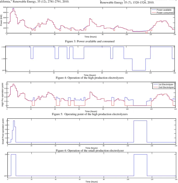
(4) PREPRINT IV.. APPLICATION. TO A CASE STUDY. A. Case study To validate the proposed control system, meteorological data in a specific location was used. In the case that 1 vertical and 1 small production electrolyzers, with an prediction horizon of 24 hours (nH = 2, nS = 1, Nh = 24). The Branch and Bound solver in the Matlab® OPTI Toolboox was used.. axes wind turbine (VAWT) and 1 wave energy converter (WEC) of those selected in the H2Ocean project provides power, a simulation has been developed for a case of 2 high. The following parameters were used to carry out the simulation and optimization:. H. Hydrogen production (Nm3).. P. Power consumption (kW).. K. Gain.. A, B. Electrolysis model constants.. S 2200 kW, Pmax = 300 kW, AH = 0.875, BH = 3.525, H S S AS = 0.778, BS = 3.622, αH i = 0.2, α i = 1, αj = 0.1, α j = 1, H K H = 608.99, K S = 81.08, λH = 1, λS = 1, λδ = 1, λδ = 1, Hmax = S 608.99, Hmax = 81.08, sampling time = 1 h.. 𝛼 α. Minimum and maximum operating points.. Hmax. Maximum hydrogen production (Nm3).. Pmax. Maximum electrolyzer power (kW).. B. Results and discussion Some partial results for 140 hours of operation are shown in Fig. 3 to 7. The results confirm the correct operation of the advanced control system for the parameters considered in the previous section. Fig. 3 shows the power provided by the renewable energy sources. Effectively, the available power is always bigger slightly than the power consumed by the electrolyzers. Power consumed has a maximum value of 4700 kW (2200 kW for each high production electrolyzer and 300 kW for the small production electrolyzer). Fig. 4 shows the performance of both high production electrolyzers. As expected, they are not switched on/off very frequently. Fig. 5 shows the operation point of these electrolyzers. In both cases, the values are between the minimum and maximum values that were defined. Finally, Fig. 6 and 7 show the operation of the small production electrolyzer. It is less connected because its performance is smaller than the performance of the high production electrolyzers. As in the previous figures, the performance of this electrolyzer can be considered correct. As can be appreciated in the simulations the controller tries to maintain the consumed power very near the available one and as consequence obtaining a hydrogen production near the achievable maximum.. Pavailable. Power available to electrolysis (kW).. λ. Weight factor.. ⃗ 1. Unit vector.. J. Cuadratic cost function.. H Pmax =. CONCLUSIONS A solution to the operation of the hybrid plant under the expected variable power supply has been presented and evaluated. Using Smart Grid ideas, a model predictive control strategy has been proposed. Simulation results based on the plant characteristics are provided to show the correct operation of the plant with the developed controller. Future research will include additional dynamic constraints in the electrolyzer operation. NOMENCLATURE H, i. High production electrolyzer subscript.. S, j. Small production electrolyzer subscript.. δ. High production binary variable.. γ. Small production binary variable.. α. Electrolyzer operating point.. ACKNOWLEDGMENT This work was funded by Ministerio de Ciencia e Innovación (Spain) under grant DPI2014-54530-R. Most of this work was carried out during a stage of A. Serna at the research group of Prof. Normey-Rico in Florianópolis (Brazil). We thank Karsten Agersted (DTU, Denmark) for his generous contribution to his work. Prof. Normey-Rico thanks CNPqBrazil for financial support. REFERENCES [1] [2]. [3] [4]. [5]. [6]. [7]. [8]. [9]. H2ocean-project.eu, (2014). H2Ocean. [online] Available at: http://www.h2ocean-project.eu/ [Accessed 28 Nov. 2014]. A. Balable, H. Kotb, “Analysis of a hybrid renewable energy standalone unit for simultaneously producing hydrogen and fresh water from sea water”. Int. J. of Thermal & Environmental Engineering, 6 (2), 5560, 2013. A. Serna, F. Tadeo, “Offshore hydrogen production from wave energy,” International Journal of Hydrogen Energy, 39 (3), 1549-1557, 2014. S.A. Sherif, F. Barbir, T.N. Veziroglu, “Wind energy and the hydrogen economy-review of the technology,” Solar energy, 78 (5), 647-660, 2005. A.G. Dutton, J.A.M. Bleijs, H. Dienhart, M. Falcheta, W. Hug, D. Prischich, A.J. Ruddell, “Experience in the design, sizing, economics, and implementation of autonomous wind-powered hydrogen production systems,” International Journal of Hydrogen Energy, 25 (8), 705-722, 2000. V. Di Bio, V. Franzitta, F. Muzio, G. Scaccianoce, M. Trapanese, “The use of sea waves for generation of electrical energy and hydrogen”, OCEANS 2009, MTS/IEEE Biloxi-Marine Technology for Our Future: Global and Local Challenges (pp1-4). IEEE, 2009. M. Momirlan, T.N. Veziroglu, “The properties of hydrogen as fuel tomorrow in sustainable energy system for a cleaner planet” International Journal of Hydrogen Energy, 30 (7), 795-802, 2005. A.A. Temeev, V.P. Belokopytov, S.A. Temeev “An integrated system of the floating wave energy converter and electrolytic hydrogen producer,” Renewable Energy, 31 (2), 225-239, 2006. D. Ghribi, A. Khelifa, S. Diaf, M. Belhamel, “Study of hydrogen production system by using PV solar energy and PEM electrolyser in Algeria”, International Journal of Hydrogen Energy, 38 (20), 8480-8490, 2013..

(5) PREPRINT [10] A.S. Joshi, I. Dincer, B.V. Reddy, “Solar energy production: A comparative performance assesstement”, International Journal of Hydrogen Energy, 36 (17), 11246-11257, 2011. [11] M.K. Deshmukh., S.S Deshmukh, “Modeling of hybrid renewable energy systems”. Renewable and Sustainable Energy Reviews, 12 (1), 235-249, 2008. [12] J.L. Bernal-Agustín, R. Dufo-López “Simulation and optimization of stand-alone hybrid renewable energy systems”, Renewable and Sustainable Energy Reviews, 13 (8), 2111-2118, 2009. [13] J.M. Carrasco, L.G. Franquelo, J.T. Bialasiewicz, E. Galván, R.P. Guisado, M.A Prats, N. Moreno-Galvan et al, “Power-electronic systems for the grid integration of renewable energy sources: A survey,” Industrial Electronics, IEEE Transactions on, 53 (4), 1002-1016, 2006. [14] E.D. Stoutenburg, N. Jenkins, M.Z. Jacobson “Power output variations of co-located offshore wind turbines and wave energy converters in California,” Renewable Energy, 35 (12), 2781-2791, 2010.. [15] O. Antonia, G. Saur “Wind to Hydrogen in California: Case Study,” National Renewable Energy Laboratory, Technical Report NREL/TP 5600-53045, 2012. [16] S.D. Ebbesen, S.H. Jensen, A. Hauch, M.B. Mogensen, “High Temperature Electrolysis in Alkaline Cells, Solid Proton Conducting Cells, and Solid Oxide Cells”, Chemical Reviews, 2014. [17] H.N. Petersen, “Note on the targeted hydrogen quality produced from electrolyser units”, Review of the Department of Energy Conversion and Storage. Technical University of Denmark, 2012. [18] E.R. Morgan, J.F. Manwell, J.G McGowan, “Opportunities for economies of scale with alkaline electrolyzers”, International Journal of Hydrogen Energy 38 (36), 15903-15909, 2013. [19] E.F. Camacho, C.B. Alba. “Model predictive control”, Springer, 2013. [20] M. Khalid, A.V. Savkin, “A model predictive control approach to the problem of wind power smoothing with controlled battery storage” Renewable Energy 35 (7), 1520-1526, 2010.. 5000. Power available Power consumed. Power (kW). 4000. 3000. 2000. 1000. 0. 0. 20. 40. 60. 80. 100. 120. 140. 100. 120. 140. Time (hours). Figure 3: Power available and consumed 2 ON. 1 ON. OFF 0. 20. 40. 60. 80. Time (hours). High Pro operation point. Figure 4: Operation of the high production electrolyzers 1. 1st Electrolyzer 2nd Electrolyzer. 0.8 0.6 0.4 0.2 0 0. 20. 40. 60. 80. 100. 120. 140. Time (hours). Small Prod operation point. Figure 5: Operating point of the high production electrolyzers 1 0.8 0.6 0.4 0.2 0 0. 20. 40. 60. 80. 100. 120. 140. 100. 120. 140. Time (hours). Figure 6: Operation of the small production electrolyzer ON. OFF 0. 20. 40. 60. 80. Time (hours). Figure 7: Operating point of the small production electrolyzer.

(6) PREPRINT ANNEX Matrix B Matrix H. Nh∙nH. Nh∙nH Nh∙nS Nh∙nH Nh∙nS. 2λH ∙ K H 2 0 0 0 0 0 0 0 0 0 0 [ 0. 0 ∙ 0 0 0 0 0 0 0 0 0 0. Nh∙nS. 0 0 0 0 ∙ 0 0 2λS ∙ K S 2 0 0 0 0 0 0 0 0 0 0 0 0 0 0 0 0. 0 0 0 0 ∙ 0 0 0 0 0 0 0. Nh∙nH. 0 0 0 0 0 0 0 0 0 0 ∙ 0 0 λδ 0 0 0 0 0 0 0 0 0 0. 0 0 0 0 0 0 0 ∙ 0 0 0 0. Pavailable (1) . . Pavailable (Nh ) 0 ∙ ∙ ∙ ∙ ∙ ∙ ∙ ∙ ∙ ∙ ∙ ∙ ∙ ∙ ∙ ∙ ∙ [ ] 0. Nh∙nS. 0 0 0 0 0 0 0 0 0 0 0 0 0 0 0 0 ∙ 0 0 λγ 0 0 0 0. 0 0 0 0 0 0 0 0 0 0 ∙ 0. 0 0 0 0 0 0 0 0 0 0 0 ∙]. Nh. Nh∙nH. Nh∙nS. Nh∙nH. Nh∙nS. Matrix 𝒇 H ∙ KH [−2λH ∙ Hmax. S −2λS ∙ Hmax ∙ KS. ⋯. Nh∙nH. ⋯. −2λδ. Nh∙nS. ⋯. −2λγ. Nh∙nH. ⋯]. 𝑇. Nh∙nS. Matrix 𝑨. Nh∙nH. Nh∙nS. Nh. Nh∙nH. Nh∙nS. Nh∙nH. Nh∙nS. ∙ ∙ 0. H Pmax ∙ ∙ ∙ ∙. H Pmax ∙. S Pmax 0 ∙ ∙ 0. 0 ∙ ∙. −1 ∙ ∙. ∙ ∙ ∙. ∙ ∙ −1. 0. ∙. ∙. ∙. 0 H Pmax. ∙ ∙ ∙. ∙ ∙ ∙. S Pmax ∙ ∙ ∙ ∙. S Pmax ∙. ∙ ∙ ∙. ∙ ∙ ∙. ∙ ∙ ∙. ∙ ∙ 0. −1. 0. ∙. ∙. 0 S Pmax. ∙ ∙ ∙. 0 ∙ ∙ ∙. ∙ ∙ ∙ ∙ 0. ∙ ∙ ∙ ∙ ∙. ∙ ∙ ∙ 0 ∙. 0 ∙ ∙ ∙ 0. ∙ ∙ ∙ ∙ ∙. ∙ ∙ ∙ ∙ ∙. ∙ ∙ ∙ 0 ∙. 0 ∙ ∙. αHi ∙ ∙. ∙ ∙ ∙. ∙ ∙. αHi. ∙ ∙ ∙. ∙ ∙ ∙. ∙ ∙ ∙. ∙ ∙ 0. 0. ∙. ∙. ∙. αSj. 0. ∙. ∙ ∙ ∙. αHi. ∙ ∙ ∙. ∙ ∙ ∙. ∙ ∙ ∙. ∙ ∙ 0. 0 ∙ ∙. −1 ∙ ∙. ∙ ∙ ∙. ∙ ∙ −1. ∙ ∙ ∙. 1. 0. ∙. ∙. 0. ∙. ∙. ∙. −α i. 0. 0 ∙ ∙. 1 ∙ ∙. ∙ ∙ ∙. ∙ ∙ 1. ∙ ∙ ∙. ∙ ∙ ∙. ∙ ∙ ∙. ∙ ∙ 0. 0 ∙ ∙. −α i ∙ ∙. 0. ∙. ∙. ∙. 1. 0. ∙. ∙. 0. ∙. ∙ ∙ [ ∙. Nh∙nS. Nh. Nh H Pmax 0 ∙ ∙ −1. Nh∙nH. ∙ ∙ ∙. ∙ ∙ ∙. ∙ ∙ 0. 0 ∙ ∙. 1 ∙ ∙. ∙ ∙ ∙. ∙ ∙ 1. ∙ ∙ ∙ H. ∙ ∙ ∙. H. ∙ ∙ ∙. ∙ ∙ ∙. ∙ ∙ ∙. 0 ∙ ∙. αSj ∙ ∙. ∙ ∙ ∙. αSj. ∙. ∙. 0. ∙. ∙. ∙. ∙ ∙ ∙. ∙ ∙. −α i. ∙ ∙ ∙. ∙ ∙ ∙. ∙ ∙ ∙. ∙ ∙ 0. ∙. ∙. −α j. ∙. ∙. ∙ ∙ ∙. ∙ ∙. ∙ ∙ ∙. ∙ ∙ 0. H. S. 0 ∙ ∙. 0 −α ∙ ∙. S j. S. −α j ].

(7)