Online machine learning algorithms to predict link quality in community wireless mesh networks
33
0
0
Texto completo
(2) services such as Internet access and voice connections [1]. In many cases, they 5. are deployed in a decentralized manner as wireless mesh networks using inexpensive networking equipment [2]. These community wireless mesh networks (CWMNs) are very dynamic, as links frequently appear and disappear, and can reach a large size. Gifui.net [3], Ninux [4], and FunkFeuer [5] are relevant examples of CWMNs in Europe.. 10. One of the most important research challenges in CWMNs is the effect of their often asymmetric and unreliable links on routing protocols and network performance [1, 6]. Link quality tracking techniques are currently employed in CWMNs to obtain metrics of the quality that can be observed in each link at a given point in time. These metrics, called Link Quality Estimators (LQEs) [7],. 15. are then used by routing protocols in CWMNs with the aim of selecting better paths. However, LQEs provide very limited information about the quality of links in the future [8], even though this information could be very useful in the context of CWMNs [6], where the quality of links can fluctuate frequently. Link quality prediction techniques can be used to forecast LQEs in CWMNs. 20. [6]. Routing protocols can leverage the information provided by link quality predictions to select routes with more reliable and stable links. With these routes, the number of packet losses and subsequent retransmissions can be reduced thus improving the network throughput [9]. Furthermore, more stable clusters can be created in the case of networks with a hierarchical topology [8].. 25. Link quality predictors should feature two important characteristics [10]. An essential requirement for a link quality predictor is adaptivity, since it should be able to adapt itself to cope with the changes in quality that might observed in the link along time. This is especially important in networks that may exhibit large dynamics, as it is the case of CWMNs. Another important feature of a. 30. link quality predictor is plug-and-play. Ideally, a link quality predictor should start working on the network without any predeployment effort since, even if the effort is reduced, it might not be feasible for all deployments. Furthermore, the availability of the predictions is delayed until the end of the predeployment. Online machine learning algorithms can be employed to build link quality 2.
(3) 35. predictors that meet both requirements [10]. These algorithms assume an initial model that can be used to generate predictions without any predeployment effort as soon as the link is up. The model can be thereafter updated every time a new quality value is observed in the link with the aim of improving the accuracy of the initial model and also adapting it to the changes observed in the link.. 40. Furthermore, online machine learning algorithms are usually designed to update models in a computational efficient way so that it can be done in real time in devices that do note feature high computational capabilities, as it is usually the case of the networking equipment employed in CWMNs. The use of link quality predictors based on online machine learning algo-. 45. rithms has already been proposed within the context of small wireless sensor networks (WSNs) [11, 10, 12] and mobile ad-hoc wireless networks (MANETs) [9]. However, to the best of our knowledge, there are no previous works that study the use of these algorithms to predict link quality in the case of large scale CWMNs.. 50. This paper explores the possibility of using online machine learning algorithms to predict link quality using real data from the FunkFeuer Wien CWMN. More specifically, the main contributions of the paper include: • A detailed analysis of the performance of 4 well-known online machine learning algorithms in the prediction of link quality in a large scale CWMN. 55. during several consecutive days, taking into account both the accuracy and the computational load generated by the algorithms, and including a comparison with a baseline. • The proposal of a new hybrid online algorithm that combines the baseline with an online machine learning algorithm to predict link quality in. 60. CWMNs. • The evaluation of the performance of the hybrid online algorithm used for link quality prediction in a large scale CWMN, including a comparison with 4 batch machine learning algorithms whose accuracy for the same prediction problem has already been studied in the literature. 3.
(4) 65. The rest of this paper is structured as follows. Section 2 discusses the related work that can be found in the literature. Next, Section 3 describes the experimental framework used in our study. Section 4 introduces the analysis of online machine learning algorithms for link quality prediction. Then, Section 5 proposes a hybrid prediction approach that combines a baseline with an. 70. online machine learning algorithm to predict link quality, evaluates its performance and compares it with that of batch machine learning algorithms. Finally, Section 6 includes the main conclusions of the paper.. 2. Related work The link quality prediction problem in CWMNs has already been addressed 75. in [6] using batch machine learning algorithms. Several well-known batch algorithms were employed to build a predictive model for each link of FunkFeuer Wien CWMN based on a set of quality values sampled from the corresponding link during an observation period of 6 days. It was also shown that the generated models performed very well in the prediction of quality values featured by. 80. links during the day right after the observation period. Unfortunately, the prediction approach followed in this work has important limitations derived from the use of batch machine learning algorithms. One of the main problems of predictive models generated using batch algorithms is that they cannot be updated once their training has been completed.. 85. This implies that they cannot be adapted to the changes that might be observed later in the link and, as a consequence, they do not perform well if the link does not behave in a similar way to the observation period, which is very likely to happen in the case of a CWMN. This is the reason why [6] observed that the mean accuracy of link quality predictions quickly decays as the difference be-. 90. tween the time for which the prediction is made and the time corresponding to the last quality value employed in building the model increases. A way of dealing with this drawback consists in building a new predictive model after the performance of the previous one has reached a given level of degradation. How-. 4.
(5) ever, this generates a higher computational load that could exceed the compu95. tational capabilities of the inexpensive networking equipment usually employed in CWMNs. Moreover, link quality predictors based on batch machine learning algorithms impose a predeployment effort: a set of quality samples must be collected in each link before building the corresponding predictions models. This is the. 100. reason why these predictors do not comply with the important plug-and-play feature [10]. It also implies that predictions are not available until the observation period is over, which might take a long time. For example, the observation period suggested in [6] to obtain the highest accuracy in predictions is 6 days long. Predictions could be generated earlier if a shorter observation period is. 105. employed, but this would reduce in many cases the generalizability of the predictive models, which in turn would lead to a significant decrease in prediction accuracy and, in any case, this would still require a predeployment effort. The use of online machine learning algorithms to predict future LQ values within the context of MANETs has been studied in [9]. More specifically, an. 110. approach was proposed to generate predictions of LQ values using the locally weighted projection regression algorithm based on past values of Received Signal Strength Indicator (RSSI) and Signal to Noise Ratio (SNR) link metrics along with the physical distance among nodes. The authors showed that their proposal generated accurate predictions using simulated data for MANETs of. 115. up to 250 moving nodes. Furthermore, they verified that their prediction approach generated a low computational load. Interestingly, they also reported that the average network throughput increased up to a 40% in the simulated MANETs when the routing protocol leveraged LQ predictions to select routes. Unlike this work, we tackle the prediction problem in a larger network in which. 120. nodes do not move. Further, we use link quality samples based on a different metric and obtained from a real network instead of from a simulated one. Other works have proposed the use of online machine learning algorithms to make link quality predictions within the context of WSNs also much smaller than the CWMN considered in our work. In [11], the prediction problem was 5.
(6) 125. casted into a classification problem in which links were given a different label (e.g. good, medium, bad) according to the values of Packet Success Rate (PSR) metric that was observed in them. Predictions in this work thus have a lower granularity than in our proposal, in which we try to predict the actual value of link quality. According to [13], predictions with higher granularity are more. 130. useful. The Temporal Adaptive Link Estimator with No Training (TALENT) [10] predicts the probability that future PSR exceeds a certain threshold using online algorithms that train predictive models using past values of PSR. Again, the granularity of predictions in this work is lower than in our case. Online algorithms were also employed in [12] to make predictions of the future Link. 135. Quality Indicator (LQI) metric that can be expected in a link. The evaluation of the proposal in this work was also made using simulations, while we use data from a real network. Besides online machine learning algorithms, the link quality prediction problem has also been dealt in in different ways for small wireless networks. For. 140. example, [14] proposes XCoPred (using Cross-Correlation to Predict), in which the nodes of a small WMN store the sequence of SNR values observed in their links so that the normalized cross correlation can then be used to find the past pattern that is most similar to the current situation. The SNR values that follow the selected pattern are employed as a prediction for the values that are. 145. expected during the next tens of seconds. The Holistic Packet Statistics (HoPs) proposed in [8] uses an exponential weighted moving average to obtain shortterm and long-term predictions of link quality based on the PSR link metric within the context of WSNs. Foresee (4C) [15] employs batch machine learning algorithms to predict the success probability of delivering the next packet ac-. 150. cording to the Received Signal Strength Indicator (RSSI), Signal to Noise Ratio (SNR) and Link Quality Indicator that can be observed in the links of WSNs. The interested reader can find in [13] the survey of more works that tackle the link quality prediction problem and are not based on online machine learning algorithms.. 155. Machine learning techniques have also been applied to address a variety 6.
(7) of problems within the context of wireless networks other than link quality prediction [16, 17, 18]. Some recent examples include intrusion detection in MANETs [19], feature selection for performance characterization in multihop WSNs [20] and efficient link quality monitoring in WSNs [21].. 160. 3. Experimental framework This section describes the framework that was employed to carry out our experiments with machine learning algorithms to predict link quality in a CWMN. This includes the dataset, the approach followed to build link quality predictors, the actual algorithms that were tested, the metrics that were employed to re-. 165. port the performance of the algorithms, the baseline that was used to facilitate the assessment of such performance, and the software and hardware that were employed to carry out the experiments. 3.1. Dataset The dataset employed in this paper comes from Funkfeuer Wien [5], a. 170. CWMN with more than 500 nodes and around 2000 links. This network uses a routing protocol that was derived from Open Link State Routing (OLSR) [22] in order to improve its scalability, which is called OLSR-Next Generation (OLSR-NG). The topology information of Funkfeuer Wien CWMN provided by OLSR-NG was collected from a node of the network every 5 minutes and pub-. 175. lished in an open data platform set by the Confine Project [23] during several years. Topology information includes the values of link quality (LQ) and neighbor link quality (NLQ) observed for all the links of the network that are active. LQ is defined as the fraction of successful probes that were received by a node. 180. from its neighbor during a certain time window, while NLQ is the fraction of successful probes received by the neighbor within the time window [22]. LQ and NLQ values can be employed to calculate the expected transmission count (ETX) [24], which can be computed as ET X = 1/(LQ × N LQ). ETX is a link. 7.
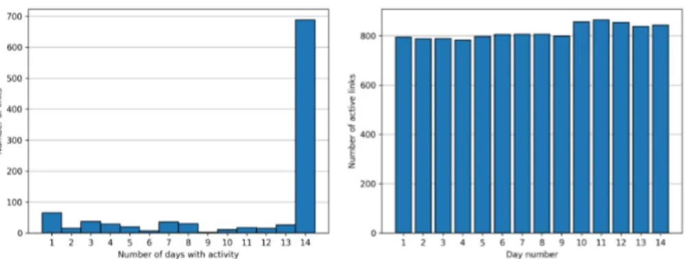
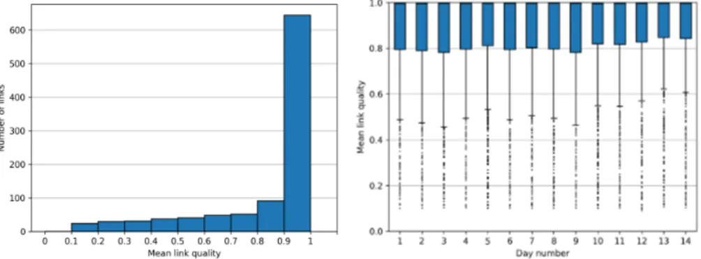
(8) metric widely employed for routing in CWMNs that estimates the total number 185. of transmissions (including retransmissions) that can be expected for a packet to be succesfully delivered over a link. Here, it can be noticed that ETX is easily obtained from LQ and NLQ, and that the NLQ of a given node can be derived from the LQ of its neighbor node. This is the reason why, same as in [6], our dataset is based on LQ values.. 190. The dataset was derived from the network topology information collected from January 15 to 28, 2016, which was available in the platform. More specifically, the dataset contains the LQ values observed for the 998 links of the network that experienced any variation in their quality during the aforementioned period of 14 days. The data of 1206 links that had constant quality were. 195. excluded from the dataset because predicting their future LQ values is trivial. It is noteworthy that the sequence of LQ values observed in each link can be considered a time series since they are a set of data collected over time with a natural ordering. In this case, the data points of the time series are LQ values ranging from 0 to 1 in the same order in which they were obtained from the. 200. link. However, it should be noticed that the difference between the times in which two consecutive LQ values were observed may vary since no observations are made when a link is off. The number of days that each link of the dataset showed activity is variable, as it can be observed in Figure 1(a). It can also be seen that most links have. 205. activity all 14 days, while the second most numerous group corresponds to links that have activity only 1 day. Figure 1(b) shows that the amount of active links per day varies around 800, which represents about 80% of the links. It is also interesting to notice in Figure 1(c) that most links are active more than 90% of the time in the days that they show activity, whereas the second largest group. 210. comprises links only active up to 10% of the time. Figure 1(d) depicts a boxplot of the percentage of time with activity for the links that show any activity in each day of the dataset. It can be observed that, except for day 13, the great majority of links are active more than 97% of the time. Concerning the quality of links, Figure 2(a) reveals that most of them have 8.
(9) (a) Number of links with respect to the num- (b) Number of links with activity in each day ber of days with activity.. of the dataset.. (c) Number of links with respect to the per- (d) Percentage of time active for links with centage of time active in days with activity.. activity in each day of the dataset.. Figure 1: Characterization of the activity of links.. 9.
(10) (a) Number of links with respect to the mean (b) Mean of LQ values in each day of the of LQ values.. dataset.. (c) Number of links with respect to the stan- (d) Standard deviation of LQ values in each dard deviation of LQ values.. day of the dataset.. Figure 2: Characterization of the quality of links.. 215. a mean quality above 0.9, while Figure 2(b) shows that the distribution of the mean quality of links with activity is quite similar in all the days of the dataset. As it can be seen in Figure 2(c), the standard deviation of quality is under 0.45 in all cases and under 0.05 in most of them. Figure 2(d) also shows that the distribution of the standard deviation of quality for the links with activity is. 220. quite similar in all days. It can also be pointed out that a strong positive correlation (r = 0.74) was found between the number of days that links showed activity and the percentage of time with activity in the days they were active. Furthermore, a moderate. 10.
(11) negative correlation (r = −0.49) was found between the mean values of link 225. quality and the standard deviation of link quality. In summary, the dataset comprises many links that were on all 14 days with a high percentage of activity and a smaller, yet significant, number of links that were off some days, and had more intermittent activity the days they were on. The unbalanced nature of the dataset makes it rather simple to achieve fair. 230. accuracy in prediction, though improving it further requires to predict well the most variable and unreliable links. 3.2. Machine learning algorithms for link quality prediction The creation and evaluation of a model to predict the value of data points in a time series such as the sequence of quality values observed in a link can be. 235. done using both online and batch machine learning algorithms. Suppose a time series made of N data points d = {d1 , d2 , ..., dN } in which predictions should be made for data points that are S steps ahead using the last W observations, which make the so-called lag window. Time series prediction with online machine learning algorithms is done fol-. 240. lowing an interleaved test and then train approach, also called prequential approach. In this approach, a set of input vectors with their corresponding output values {< (di−W +1 , ..., di−1 , di ), di+S >: i = W, ..., (N − S)} is derived from the time series. Each input vector is first employed to get the predicted output from the model. Next, the same input vectors are used along with its correspond-. 245. ing actual output to update the model. The predictions obtained in this way can also be compared with the actual output values in order to determine the accuracy of the model. One of the main advantages of online machine learning algorithms is the possibility of updating the prediction model every time a new data point is. 250. available. Furthermore, the computational load generated by online algorithms is often much low since each update of the model implies the use of just one input vector along with its corresponding output. This facilitates the possibility of running the algorithms in the network nodes that feature low computational 11.
(12) capabilities. 255. In this paper, 4 well-known online machine learning algorithms for regression are employed to make one step ahead predictions of the series of LQ values corresponding to each link of the dataset: online perceptron [25] (OP), online regression trees with options (ORTO) [26], fast incremental model trees with drift detection (FIMT-DD) [27], and adaptive model rules (AMRules) [28].. 260. Any of these algorithms can be employed to generate predictions for all of the 14 days of the dataset. However, it is well known that the performance of these algorithms in the prediction of the first samples of a time series cannot be considered representative of the performance that can be achieved in the long term, which is due to the fact that the model used to generate the first. 265. predictions has been trained with very few samples. This is the reason why the first day of the dataset was used in our experiments only to train models, while the remaining 13 days were employed both to test and train the models. In the case of batch machine learning algorithms, time series prediction requires deriving a training set and a test set from the series. If the first P ≥. 270. W +S data points shall be employed to create a prediction model, then a training set consisting of pairs of input vectors with their corresponding output values {< (di−W +1 , ..., di−1 , di ), di+S >: i = W, ..., (P − S)} can be derived from the time series. Similarly, if the next Q data points shall be employed to evaluate the prediction model, then a test set also consisting in pairs of input vectors. 275. with their corresponding output values {< (di−W +1 , ..., di−1 , di ), di+S >: i = (P − S + 1), ..., (N − S)} can be derived. If desired, feature selection methods could be used with the training set to reduce the size of vectors in both sets. Another option would be to extend vectors of both sets with additional features such as, for example, the date or time of the observations.. 280. Creating a predictive model with a batch machine learning algorithm usually requires multiple iterations of the algorithm over the whole training set. This is the reason why some batch algorithms can be very demanding from a computational point of view. Once the model has been generated, it can be employed to predict the output values corresponding to the input vectors of the 12.
(13) 285. test set. Then, the predictions can be compared with the actual output values of the test set in order to determine the accuracy of the model. In a real setting, only the data points available at a given time can be used to create a predictive model with batch machine learning algorithms. The model can then be used to predict future data points. However, if the underlying. 290. data distribution evolved, the prediction quality of the model decreases, since it predicts according to past knowledge that is no longer accurate. Unfortunately, the model cannot be updated with each new data point that becomes available. In this way, a new model must be created using the data available some time after the generation of the previous model. This significantly increases the. 295. computational load required to make link quality predictions, thus hindering the possibility of running the algorithms in network nodes that feature low computational capabilities. This paper uses for comparison purposes the same 4 well-known batch machine learning algorithms for regression that were studied in [6] to make also. 300. one step ahead predictions of LQ values: Support Vector Machines (SVM) [29], k-Nearest Neigbours (kNN) [30], Regression Trees (RT) based on reduced error pruning [31], and Gaussian Processes for Regression (GPR) [32]. According to [6], the LQ values observed in a link during 6 days in a row should be used with a lag window of size 12, corresponding to the LQ values observed in the last hour,. 305. when creating a model with any of these batch algorithms to make predictions one step ahead during the next day. This implies that a new model must be trained for every test day using the most recent data available. Following this approach, in our experiments each batch algorithm was used with a lag window size of 12 to train a different predictive model for each of the days 7 to 14 using. 310. the LQ values available from the 6 previous days right after the end of days 6 to 13, respectively. The models were then employed to generate the predictions of LQ values expected for each link during days 7 to 14. Moreover, it was verified in [6] that the accuracy of the models could be improved by saturating the predicted values so that all predictions above 1 would be 1, and all predictions. 315. below 0 would be 0. This improvement was also included in our experiments. 13.
(14) 3.3. Performance metrics and baseline Two aspects of the performance of machine learning algorithms in the prediction of LQ values are evaluated in this paper. One is the accuracy of the predictions made by the algorithms; the other is the computational load gener320. ated by the the training and testing of the algorithms. Mean Average Error (MAE) and Root Mean Squared Error (RMSE) are two metrics usually employed to evaluate the accuracy of prediction methods in time series analysis [33]. However, RMSE is more sensitive to outliers, which has led some authors such as [34] to recommend against its use in time series prediction. 325. evaluation. This is the reason why MAE is used in this paper to measure the accuracy of machine learning algorithms. The computational load generated by machine learning algorithms is usually evaluated (e.g. [25], [26], [27], [28]) using the CPU time that is consumed by the execution of the algorithms. CPU time is also the metric employed in this. 330. paper to measure computational load. The accuracy and computational load of a simple baseline prediction algorithm are also reported in this paper in order to facilitate the assessment of the performance of machine learning algorithms. Here we propose a simple baseline that predicts that the next LQ value will be the same as the last measured. 335. value. 3.4. Experimental environment The experiments reported in this paper used the Java implementations of online and batch machine learning algorithms provided by, respectively, the 2016.04 release of the Massive Online Analysis framework [35] for data streams,. 340. and version 3.8.1 of Weka data mining software [36]. All experiments were run on a single CPU Intel Core i7 3615 QM with 4 cores and 16GB of RAM. However, it should be taken into account that the networking equipment available in CWMNs is usually inexpensive and, when that is the case, more CPU time would be needed to complete the training of the models and to make the predictions. 345. using them. 14.
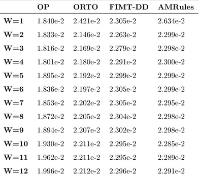
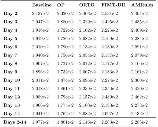
(15) 4. Analysis of online machine learning algorithms The analysis introduced in this section aims at determining if the online machine learning algorithms under study can improve the accuracy of the baseline algorithm as well as to understand if the accuracy of the algorithms depends 350. on the activity of the links or the quality that can be observed in the links. Furthermore, it seeks to assess the computational load that algorithms generate. However, to carry out this analysis, it was necessary to first determine the size of the lag window to be used for the testing and training of the prediction models generated with each online machine learning algorithm.. 355. 4.1. Lag window size The impact that the size of lag window has in the accuracy of online machine learning algorithm was checked in order to determine the size to be used with each of them. Table 1 shows the MAE of all predictions made for days 2 to 14 using each online algorithm with lag window sizes ranging from 1 to 12. It can. 360. be seen that the best results are achieved with lag window size 4 for OP, 2 for ORTO and FIMT-DD, and 10 in the case of AMRules. It is worth mentioning that the differences between the best MAE and second best MAE with respect to size of lag window for each algorithm are statistically significant (p < 0.01) in all cases.. 365. Here, it should be noticed that rest of the results reported in this section are based on experiments made with the lag window sizes that get the best results for each algorithm. 4.2. Prediction accuracy The MAE of predictions corresponding to each day 2 to 14 as well as the. 370. MAE of all predictions that can be achieved with the baseline and each online algorithm are shown in Table 2. It can be seen that the results of the baseline algorithm are better than those of ORTO, FIMT-DD and AMRules. The differences between the accuracy of baseline and those three algorithms are statistically significant (p < 0.01) in all cases. Only OP outperforms the baseline 15.
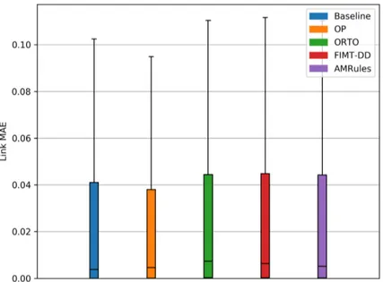
(16) OP. ORTO. FIMT-DD. AMRules. W=1. 1.840e-2. 2.421e-2. 2.305e-2. 2.634e-2. W=2. 1.833e-2. 2.146e-2. 2.263e-2. 2.299e-2. W=3. 1.816e-2. 2.169e-2. 2.279e-2. 2.298e-2. W=4. 1.801e-2. 2.180e-2. 2.291e-2. 2.300e-2. W=5. 1.895e-2. 2.192e-2. 2.299e-2. 2.299e-2. W=6. 1.836e-2. 2.197e-2. 2.305e-2. 2.299e-2. W=7. 1.853e-2. 2.202e-2. 2.305e-2. 2.295e-2. W=8. 1.872e-2. 2.205e-2. 2.304e-2. 2.298e-2. W=9. 1.894e-2. 2.207e-2. 2.302e-2. 2.298e-2. W=10. 1.930e-2. 2.211e-2. 2.295e-2. 2.285e-2. W=11. 1.962e-2. 2.211e-2. 2.295e-2. 2.289e-2. W=12. 1.996e-2. 2.212e-2. 2.296e-2. 2.291e-2. Table 1: Overall MAE of predictions made by each online machine learning algorithm for days 2 to 14 with respect to lag window size.. 375. every day, being all differences also statistically significant (p < 0.01). It is also noteworthy that OP improves the baseline overall MAE by 8.9%. Figure 3 depicts the boxplot of MAE corresponding to all predictions made for each link using the baseline and each online algorithm. It can be seen that the median value is lower for the baseline than for any other algorithm, while. 380. the value of its third quartile is higher than for OP but lower than for the rest of the algorithms. This implies that, in spite of OP having a better overall MAE, there are links in which predictions made with baseline were more accurate. The second and third quartiles are also lower for OP than for ORTO, FIMT-DD and AMRules.. 385. 4.3. Impact of link activity in prediction accuracy The boxplots in Figure 4 reveal that the performance of all algorithms is clearly worse when the link is active only 1 or 2 days. Here, it must be taken into account that these links not only are active during very few days, but 16.
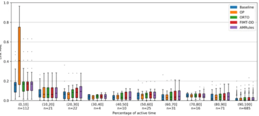
(17) Baseline. OP. ORTO. FIMT-DD. AMRules. Day 2. 2.137e-2. 2.020e-2. 2.403e-2. 2.531e-2. 2.494e-2. Day 3. 2.047e-2. 1.880e-2. 2.320e-2. 2.425e-2. 2.435e-2. Day 4. 1.916e-2. 1.722e-2. 2.102e-2. 2.225e-2. 2.409e-2. Day 5. 1.919e-2. 1.726e-2. 2.082e-2. 2.169e-2. 2.284e-2. Day 6. 2.010e-2. 1.790e-2. 2.134e-2. 2.180e-2. 2.091e-2. Day 7. 1.940e-2. 1.756e-2. 2.054e-2. 2.137e-2. 2.079e-2. Day 8. 1.907e-2. 1.727e-2. 2.072e-2. 2.177e-2. 2.106e-2. Day 9. 1.896e-2. 1.732e-2. 2.067e-2. 2.183e-2. 2.161e-2. Day 10. 2.011e-2. 1.874e-2. 2.096e-2. 2.274e-2. 2.360e-2. Day 11. 2.018e-2. 1.861e-2. 2.239e-2. 2.350e-2. 2.420e-2. Day 12. 1.989e-2. 1.793e-2. 2.157e-2. 2.489e-2. 2.462e-2. Day 13. 1.966e-2. 1.775e-2. 2.100e-2. 2.183e-2. 2.273e-2. Day 14. 1.941e-2. 1.762e-2. 2.082e-2. 2.097e-2. 2.132e-2. Days 2-14. 1.977e-2. 1.801e-2. 2.146e-2. 2.263e-2. 2.285e-2. Table 2: Daily MAE and overall MAE of predictions made by baseline and each online machine learning algorithm for days 2 to 14.. also a very low percentage of time in those days, as it was already shown by the 390. strong correlation between the number of days that links showed activity and the percentage of active time. This implies that the number of LQ values observed in those links is low, which hinders the possibility of training accurate predictive models. The problem is much worse in the case of OP because, unlike the rest of the online algorithms, it cannot start updating the prediction model until. 395. W + 1 LQ values are available and, in the meantime, it generates predictions with value 0. It can also be observed in the boxplots depicted in Figure 5 that the performance of all algorithms is significantly worse in the case of links that feature up to a 10% of active time on average during the days in which they show activity.. 400. Many links of this group were active only during 1 or 2 days, and the reasons for the low accuracy in this case have already been explained. There are also 17.
(18) Figure 3: Distribution of link MAE of predictions made by baseline and each online machine learning algorithms for days 2 to 14. Outliers are not shown to improve the readability of the figure.. Figure 4: Distribution of link MAE of predications made by baseline and each online machine learning algorithms for days 2 to 14 with respect to the number of active days.. links in this group that were active during more than 2 days. However, these links were often turned off, which implies that the difference of time between two consecutive LQ values observed is high in many cases. Again, this hinders 405. the possibility of training accurate predictive models. The especially poor performance of OP with this group of links can also be attributed to the predictions. 18.
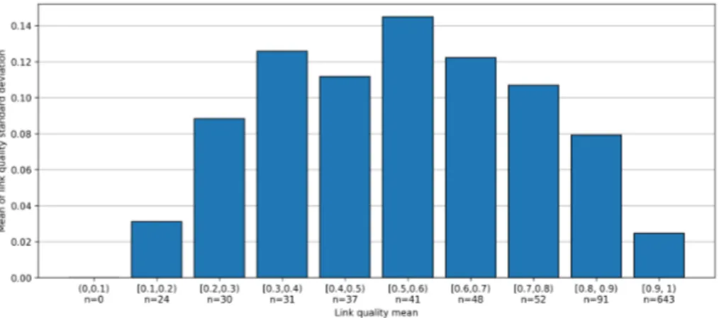
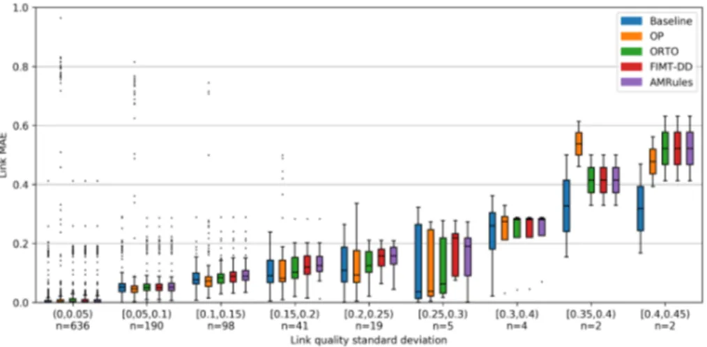
(19) Figure 5: Distribution of link MAE of predications made by baseline and each online machine learning algorithms for days 2 to 14 with respect to the percentage of active time.. with value 0 that it generates until it starts training a model. 4.4. Impact of link quality in prediction accuracy There is no apparent relationship between the performance of algorithms 410. and the mean quality of the links for which predictions are generated according to Figure 6. However, if the mean standard deviation in LQ of the links corresponding to each group is taken into account, which is shown in Figure 7, it can be observed that the performance of algorithms with each group of links is clearly related.. 415. The relationship between the performance of algorithms and link quality standard deviation can also be confirmed with Figure 8. It can be seen that the performance of all algorithms decreases with the standard deviation of link groups in the range (0, 0.25); groups in the range [0.25, 0.45) should not be taken into account since the number of links in each of them is very low. Moreover, it. 420. can be noticed that OP performs better than any other algorithm in the groups of links within the range (0.05, 0.25), while the baseline performs better in the group with links quality standard deviation ranging in (0, 0.05), i.e. the most stable links.. 19.
(20) Figure 6: Distribution of link MAE achieved by baseline and online machine learning algorithms for days 2 to 14 with respect to the mean of LQ values in each link.. Figure 7: Mean of link quality standard deviation corresponding to groups of links made according to their mean link quality.. 4.5. Computational load 425. We measured the CPU time that was employed in each test day 2 to 14 by each online algorithm to generate the predictions and to update the models. The time employed by the baseline to generate the predictions for the same days was measured too. The mean CPU time per day corresponding to each algorithm can be seen in Table 3. As expected, the baseline is the algorithm. 430. that requires less CPU time. However, it is noteworthy that OP, ORTO and. 20.
(21) Figure 8: Distribution of link MAE achieved by baseline and online machine learning algorithms for days 2 to 14 with respect to the standard deviation of LQ values in each link.. Test & train. Baseline. OP. ORTO. FIMT-DD. AMRules. 0.02. 0.35. 0.24. 0.26. 10.46. Table 3: Mean CPU time (in seconds) per day employed by the baseline to generate the predictions and by each online machine learning algorithm to generate the predictions and update the models for days 2 to 14.. FIMT-DD required on average less than 0.5 seconds per day. AMRules was more demanding from a computational point of view although the load it generates can also be considered low. 4.6. Lessons learned 435. The analysis of online machine learning algorithms detailed in this section allowed us to draw the following conclusions: • OP is the only online machine learning algorithm that outperforms the baseline in terms of accuracy. • The accuracy of OP is hindered by the predictions with value 0 that are. 440. generated until W + 1 LQ values are available to start updating a model.. 21.
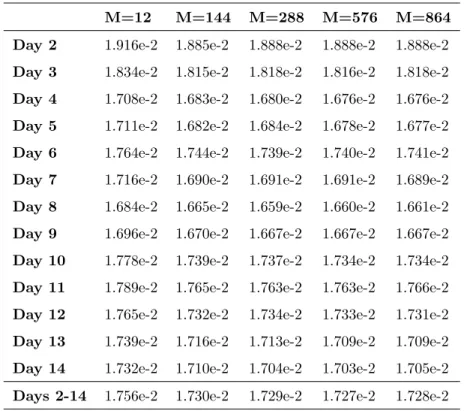
(22) • The baseline performs better than OP in some cases, including links with low standard deviation of their quality. • The computational demands of OP are very light. Based on these observations, it seems reasonable to expect that baseline and 445. OP algorithms could be combined in an attempt to improve the accuracy of any of them while keeping the computational demands low.. 5. A hybrid online algorithm for the prediction of link quality We propose a hybrid online algorithm that combines the use of baseline and OP as described next. Suppose that the hybrid online algorithm is employed to 450. make predictions for a link using a lag window of size W , an accuracy window of size M and, at a given time, P observations of LQ values have already been made. If P < W + 1, then the baseline method shall be employed to generate a prediction. If P ≥ W + 1, then the algorithm that achieved the lowest MAE with its predictions for the last min(M, P − W − 1) data points shall be used.. 455. With this hybrid model, a sensible prediction will be made at any time, regardless of the number of data points already observed. Moreover, if the OP is performing well in the past, presumably because it has captured well the variations of the underlying distribution, it will be used. If, on the contrary, the baseline is doing better, most likely because the link is very stable, it will be. 460. preferred. It should be noticed that this selection is dynamic in nature, being automatically updated after every observation. 5.1. Prediction accuracy The hybrid online algorithm was employed to make all predictions for days 2 to 4 using lag window size 4 and accuracy window sizes 12, 144, 288, 576, and. 465. 864 which correspond to the number of samples that can be collected from a link that is continuously active during 0.5, 1, 2, and 3 days respectively. Table 4 shows the MAE of predictions corresponding to each day as well as the MAE of all predictions that were obtained. It can be observed that the accuracy 22.
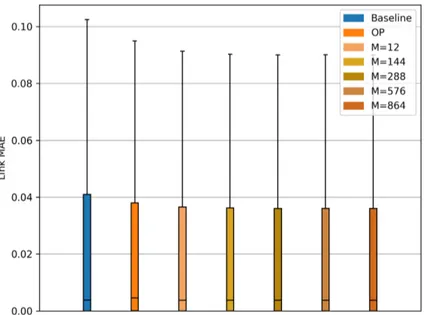
(23) M=12. M=144. M=288. M=576. M=864. Day 2. 1.916e-2. 1.885e-2. 1.888e-2. 1.888e-2. 1.888e-2. Day 3. 1.834e-2. 1.815e-2. 1.818e-2. 1.816e-2. 1.818e-2. Day 4. 1.708e-2. 1.683e-2. 1.680e-2. 1.676e-2. 1.676e-2. Day 5. 1.711e-2. 1.682e-2. 1.684e-2. 1.678e-2. 1.677e-2. Day 6. 1.764e-2. 1.744e-2. 1.739e-2. 1.740e-2. 1.741e-2. Day 7. 1.716e-2. 1.690e-2. 1.691e-2. 1.691e-2. 1.689e-2. Day 8. 1.684e-2. 1.665e-2. 1.659e-2. 1.660e-2. 1.661e-2. Day 9. 1.696e-2. 1.670e-2. 1.667e-2. 1.667e-2. 1.667e-2. Day 10. 1.778e-2. 1.739e-2. 1.737e-2. 1.734e-2. 1.734e-2. Day 11. 1.789e-2. 1.765e-2. 1.763e-2. 1.763e-2. 1.766e-2. Day 12. 1.765e-2. 1.732e-2. 1.734e-2. 1.733e-2. 1.731e-2. Day 13. 1.739e-2. 1.716e-2. 1.713e-2. 1.709e-2. 1.709e-2. Day 14. 1.732e-2. 1.710e-2. 1.704e-2. 1.703e-2. 1.705e-2. Days 2-14. 1.756e-2. 1.730e-2. 1.729e-2. 1.727e-2. 1.728e-2. Table 4: Daily MAE and overall MAE of predictions made by hybrid online algorithm for days 2 to 14 with respect to accuracy window size.. improves with size 144 with respect to size 12. Sizes 288, 576, and 864 feature 470. marginally lower accuracies when compared with size 144. It is noteworthy that MAE values achieved by the hybrid online algorithm with any accuracy window size are lower every day than those obtained with OP. The differences between the accuracies of both algorithms are statistically significant (p < 0.01). The hybrid online algorithm with accuracy window size. 475. 144 improves the OP overall MAE by 3.9% and the baseline overall MAE by 12.5%. The boxplot of MAE corresponding to all predictions made for each link of the dataset made with the hybrid online algorithm is depicted in Figure 9. The second and third quartiles are lower for the hybrid online algorithm with any. 480. accuracy window size than for the baseline or OP. The upper inner fence Q3 + 1.5IQ is also lower for the hybrid online algorithm also regardless of the accuracy 23.
(24) Figure 9: Distribution of link MAE of predictions made by baseline, OP and hybrid online machine learning algorithm for days 2 to 14. Outliers are not shown to improve the readability of the figure.. window size. Both facts support the idea that the hybrid online algorithm has an overall better performance in terms of accuracy than the baseline and OP. Here it can be recalled that OP is an algorithm that performs clearly better 485. than the baseline with links that do not feature a very low standard deviation of quality. Hence, it can be expected that the proposed hybrid online algorithm achieves a much better accuracy than the baseline in the case of CWMNs where the percentage of links with variable quality is higher than in our dataset. 5.2. Computational load. 490. Again, we measured the CPU time that was used in each test day 2 to 14 by the hybrid online algorithm to generate predictions and train the predictive models. The mean CPU time per day obtained with each accuracy window size is shown in Table 5. As expected, the time increases with the size of the accuracy window. In any case, the computational demands of all options are. 495. low. 24.
(25) Test & train. M=12. M=144. M=288. M=576. M=864. 0.47. 0.75. 1.37. 2.60. 3.59. Table 5: Mean CPU time (in seconds) per day employed by the hybrid online machine learning algorithm to generate the predictions and update the models for days 2 to 14 with respect to the accuracy window size.. Interestingly, the time required in the case of M = 288 nearly doubles the time employed with M = 144. Given the marginal difference of accuracy between both options, it seems reasonable to choose M = 144 as a good compromise option. 500. 5.3. Comparison with batch algorithms An important limitation of batch machine learning algorithms for the prediction of link quality that was already reported in [6] is that they cannot be used unless there are a minimum of W + 1 LQ values available to generate a training set. This implies that, unlike in the case of the hybrid online algorithm. 505. proposed in this paper, no predictions can be made for links when it is their first day of activity or if they have been active for a very short time in the previous 6 days. Figure 10 shows the percentage of active links during days 7 to 14 of our dataset for which it is not possible to generate predictions using batch machine learning algorithms. It is noteworthy that this percentage is as high as 8.4%. 510. in day 10. In the experiment reported next, this limitation was circumvented by using the baseline algorithm to obtain predictions in the cases in which a predictive model generated with batch algorithms is not available. Table 6 shows the MAE of predictions corresponding to each day 7 to 14 along with the MAE of all predictions for those days that can be obtained with. 515. the baseline, the hybrid online algorithm with accuracy window size 144, and each batch machine leaning algorithm combined with the baseline. It can be seen that both the hybrid online algorithm and the baseline clearly outperform kNN, RT and GPR every day. These differences are statistically significant (p < 0.01) in all cases. It is also noteworthy that there are some days in which. 25.
(26) Figure 10: Percentage of active links during days 7 to 14 that do not get any prediction from batch algorithms.. 520. the hybrid online algorithm performs better than SVM, while other days it is the other way round. However, in this case not all the differences are statistically significant. In fact, the difference between the overall MAE achieved by the hybrid online algorithm and SVM is not statistically significant (p = 0.704) either. In this way, it is possible to state that both algorithms have a similar. 525. overall performance in terms of accuracy. Table 7 compares the mean CPU time per day required by the hybrid online algorithm and the batch machine learning algorithms to train the models and use them to generate predictions for days 7 to 14. It can be seen kNN and RT employed reasonably low CPU times, while SVM was quite demanding and. 530. GRP generated a very high computational load. The hybrid online algorithm proposed here generated a computational load lower than any batch machine learning algorithm. In fact, it is noteworthy that the mean CPU time per day employed by the hybrid online algorithm represents only 0.1% of the time. 26.
(27) Baseline. Hybrid. SVM. kNN. RT. GPR. Day 7. 1.940e-2. 1.690e-2. 1.645e-2. 1.962e-2. 2.051e-2. 2.475e-2. Day 8. 1.907e-2. 1.665e-2. 1.699e-2. 1.970e-2. 2.049e-2. 2.501e-2. Day 9. 1.896e-2. 1.670e-2. 1.676e-2. 1.968e-2. 2.078e-2. 2.523e-2. Day 10. 2.011e-2. 1.739e-2. 1.686e-2. 2.021e-2. 2.403e-2. 2.731e-2. Day 11. 2.018e-2. 1.765e-2. 1.898e-2. 2.122e-2. 2.247e-2. 2.984e-2. Day 12. 1.989e-2. 1.732e-2. 1.724e-2. 2.072e-2. 2.082e-2. 3.113e-2. Day 13. 1.966e-2. 1.716e-2. 1.701e-2. 2.031e-2. 2.103e-2. 2.631e-2. Day 14. 1.941e-2. 1.710e-2. 1.640e-2. 1.969e-2. 2.023e-2. 2.625e-2. Days 7-14. 1.959e-2. 1.730e-2. 1.710e-2. 2.015e-2. 2.130e-2. 2.702e-2. Table 6: Daily MAE and overall MAE of predictions made by baseline, hybrid online algorithm and batch machine learning algorithms combined with baseline for days 7 to 14.. Train & test. Baseline. Hybrid. SVM. kNN. RT. GPR. 0.02. 0.77. 733.56. 120.89. 34.36. 5841.37. Table 7: Mean CPU time (in seconds) per day employed by the baseline to generate the predictions, the hybrid online algorithm and batch machine learning algorithms combined with baseline to train and test the models for days 7 to 14.. required by SVM. 535. In summary, SVM is the only batch machine learning algorithm that achieves an accuracy similar to that of the hybrid online algorithm. However, the computational load generated by the latter is much lower. The hybrid online algorithm should thus be preferred to make predictions of link quality in a CWMN since the networking equipment in these networks is usually inexpensive and features. 540. low computational capabilities.. 6. Conclusions The potential benefits of accurate link quality prediction in CWMNs include improved network throughput and more stable clusters in hierarchical topologies. Unlike batch machine learning algorithms, online machine learning 27.
(28) 545. algorithms can be used to build link quality predictors that automatically adjust themselves to cope with changes in the links and that do not require efforts that hinder or even preclude their deployment. However, the use of online machine learning algorithms to make link quality predictions in CWMNs has not been explored yet.. 550. In this paper we studied the performance of 4 well-known online machine learning algorithms for link quality prediction in terms of accuracy and computational load using data from a real CWMN. It was observed that only one of them, OP, outperforms the accuracy of a simple baseline. Furthermore, it was shown that OP generates a low computational load. Moreover, the analysis. 555. of the impact of link activity and link quality in the accuracy of both baseline and OP allowed us to understand the circumstances in which each algorithm performs better. Based on this analysis, we proposed a hybrid algorithm that combines OP and the baseline. This hybrid online machine learning algorithm improved the accuracy of the baseline by a 12.5% while generating a reasonably. 560. low computational load. The improvement is expected to be even better in the case of CWMNs with a higher percentage of links in which quality varies frequently. We also compared the performance of the proposed algorithm with that of 4 batch machine learning algorithms to predict link quality in a CWMN. Firstly,. 565. it was observed that, using batch algorithms, it was not possible to generate predictions for links when it is their first day of activity or if they have been active for a very short time in the previous days. However, we circumvented this problem by using the baseline to generate predictions in those cases in order to make the comparison with online machine learning algorithms. The. 570. results of the experiments showed that SVM is is the only batch machine learning algorithm that yields an accuracy similar to that of the proposed hybrid online algorithm. However, the proposed algorithm requires only 0.1% of the computational load generated by SVM. The rest of the batch machine learning algorithms feature worse accuracy than the baseline.. 575. Regarding future work, the performance of the hybrid online machine learn28.
(29) ing algorithm will be evaluated using data of other CWMNs with a higher number of links and a higher percentage of variable links. There are also plans to study the improvement of the throughput that can be achieved in a CWMN when OLSR is used along with the link quality predictions made by the hybrid 580. online algorithm.. Acknowledgements This work has been partially funded by the Spanish Ministry of Economy and Competitiveness (project TIN2014-53199-C3-2-R) and the Regional Government of Castilla y León (project VA082U16).. 585. References [1] B. Braem, C. Blondia, C. Barz, H. Rogge, F. Freitag, L. Navarro, J. Bonicioli, S. Papathanasiou, P. Escrich, R. Baig Viñas, A. L. Kaplan, A. Neumann, I. Vilata i Balaguer, B. Tatum, M. Matson, A case for research with and on community networks, ACM SIGCOMM Computer Communication. 590. Review 43 (3) (2013) 68–73. doi:10.1145/2500098.2500108. [2] P. A. Frangoudis, G. C. Polyzos, V. P. Kemerlis, Wireless community networks: an alternative approach for nomadic broadband network access, IEEE Communications Magazine 49 (5) (2011) 206–213. doi:10.1109/ MCOM.2011.5762819.. 595. [3] R. Baig, R. Roca, F. Freitag, L. Navarro, guifi.net, a crowdsourced network infrastructure held in common, Computer Networks 90 (2015) 150 – 165, crowdsourcing. doi:0.1016/j.comnet.2015.07.009. [4] L. Maccari, An analysis of the Ninux wireless community network, in: IEEE 9th International Conference on Wireless and Mobile Computing, Network-. 600. ing and Communications (WiMob), 2013, pp. 1–7. doi:10.1109/WiMOB. 2013.6673332.. 29.
(30) [5] Funkfeuer [online, visited on 28/03/17]. URL www.funkfeuer.at [6] P. Millan, C. Molina, E. Medina, D. Vega, R. Meseguer, B. Braem, 605. C. Blondia, Time series analysis to predict link quality of wireless community networks, Computer Networks 93, Part 2 (2015) 342 – 358. doi: 10.1016/j.comnet.2015.07.021. [7] N. Baccour, A. Koubâa, L. Mottola, M. A. Zúñiga, H. Youssef, C. A. Boano, M. Alves, Radio link quality estimation in wireless sensor networks:. 610. A survey, ACM Trans. Sen. Netw. 8 (4) (2012) 34:1–34:33. doi:10.1145/ 2240116.2240123. [8] C. Renner, S. Ernst, C. Weyer, V. Turau, Prediction accuracy of linkquality estimators, in:. P. J. Marrón, K. Whitehouse (Eds.), Wire-. less Sensor Networks: 8th European Conference, EWSN 2011, Springer 615. Berlin Heidelberg, Berlin, Heidelberg, 2011, pp. 1–16.. doi:10.1007/. 978-3-642-19186-2_1. [9] G. A. D. Caro, M. Kudelski, E. F. Flushing, J. Nagi, I. Ahmed, L. M. Gambardella, Online supervised incremental learning of link quality estimates in wireless networks, in: 2013 12th Annual Mediterranean Ad 620. Hoc Networking Workshop (MED-HOC-NET), 2013, pp. 133–140. doi: 10.1109/MedHocNet.2013.6767422. [10] T. Liu, A. E. Cerpa, Temporal adaptive link quality prediction with online learning, ACM Trans. Sen. Netw. 10 (3) (2014) 46:1–46:41. doi:10.1145/ 2594766.. 625. [11] Y. Wang, M. Martonosi, L.-S. Peh, Predicting link quality using supervised learning in wireless sensor networks, SIGMOBILE Mob. Comput. Commun. Rev. 11 (3) (2007) 71–83. doi:10.1145/1317425.1317434. [12] D. Marinca, P. Minet, On-line learning and prediction of link quality in. 30.
(31) wireless sensor networks, in: 2014 IEEE Global Communications Confer630. ence, 2014, pp. 1245–1251. doi:10.1109/GLOCOM.2014.7036979. [13] C. J. Lowrance, A. P. Lauf, Link quality estimation in ad hoc and mesh networks: A survey and future directions, Wireless Personal Communications 96 (1) (2017) 475–508. doi:10.1007/s11277-017-4180-9. [14] K. Farkas, T. Hossmann, F. Legendre, B. Plattner, S. K. Das, Link quality. 635. prediction in mesh networks, Computer Communications 31 (8) (2008) 1497 – 1512, special Issue: Modeling, Testbeds, and Applications in Wireless Mesh Networks. doi:10.1016/j.comcom.2008.01.047. [15] T. Liu, A. E. Cerpa, Data-driven link quality prediction using link features, ACM Trans. Sen. Netw. 10 (2) (2014) 37:1–37:35. doi:10.1145/2530535.. 640. [16] A. Forster, Machine learning techniques applied to wireless ad-hoc networks: Guide and survey, in: 2007 3rd International Conference on Intelligent Sensors, Sensor Networks and Information, 2007, pp. 365–370. doi:10.1109/ISSNIP.2007.4496871. [17] R. V. Kulkarni, A. Forster, G. K. Venayagamoorthy, Computational intelli-. 645. gence in wireless sensor networks: A survey, IEEE Communications Surveys Tutorials 13 (1) (2011) 68–96. doi:10.1109/SURV.2011.040310.00002. [18] M. A. Alsheikh, S. Lin, D. Niyato, H. P. Tan, Machine learning in wireless sensor networks: Algorithms, strategies, and applications, IEEE Communications Surveys Tutorials 16 (4) (2014) 1996–2018. doi:10.1109/COMST.. 650. 2014.2320099. [19] E. A. Shams, A. Rizaner, A novel support vector machine based intrusion detection system for mobile ad hoc networks, Wireless Networksdoi:10. 1007/s11276-016-1439-0. [20] A. Panousopoulou, M. Azkune, P. Tsakalides, Feature selection for per-. 655. formance characterization in multi-hop wireless sensor networks, Ad Hoc. 31.
(32) Networks 49 (Supplement C) (2016) 70 – 89. doi:https://doi.org/10. 1016/j.adhoc.2016.06.011. [21] E. Ancillotti, C. Vallati, R. Bruno, E. Mingozzi, A reinforcement learningbased link quality estimation strategy for RPL and its impact on topology 660. management, Computer Communications 112 (Supplement C) (2017) 1 – 13. doi:10.1016/j.comcom.2017.08.005. [22] T. Clausen, P. Jacquet, Optimized Lins State Routing protocol (OLSR), RFC 3626, RFC Editor (2003). [23] Confine project [online, visited on 01/03/2017].. 665. URL https://confine-project.eu [24] D. S. J. De Couto, D. Aguayo, J. Bicket, R. Morris, A high-throughput path metric for multi-hop wireless routing, in: 9th Annual International Conference on Mobile Computing and Networking, MobiCom ’03, ACM, New York, NY, USA, 2003, pp. 134–146. doi:10.1145/938985.939000.. 670. [25] A. Bifet, G. Holmes, B. Pfahringer, E. Frank, Fast perceptron decision tree learning from evolving data streams, in: 14th Pacific-Asia Conference on Advances in Knowledge Discovery and Data Mining - Volume Part II, PAKDD’10, Springer-Verlag, Berlin, Heidelberg, 2010, pp. 299–310. doi: 10.1007/978-3-642-13672-6_30.. 675. [26] E. Ikonomovska, J. Gama, B. Zenko, S. Dzeroski, Speeding-up hoeffdingbased regression trees with options, in: L. Getoor, T. Scheffer (Eds.), 28th International Conference on Machine Learning, Omnipress, 2011, pp. 537– 544. [27] E. Ikonomovska, J. Gama, S. Džeroski, Learning model trees from evolving. 680. data streams, Data Mining and Knowledge Discovery 23 (1) (2011) 128– 168. doi:10.1007/s10618-010-0201-y.. 32.
(33) [28] J. Duarte, J. Gama, A. Bifet, Adaptive model rules from high-speed data streams, ACM Trans. Knowl. Discov. Data 10 (3) (2016) 30:1–30:22. doi: 10.1145/2829955. 685. [29] S. K. Shevade, S. S. Keerthi, C. Bhattacharyya, K. R. K. Murthy, Improvements to the SMO algorithm for SVM regression, IEEE Transactions on Neural Networks 11 (5) (2000) 1188–1193. doi:10.1109/72.870050. [30] D. W. Aha, D. Kibler, M. K. Albert, Instance-based learning algorithms, Machine Learning 6 (1) (1991) 37–66. doi:10.1007/BF00153759.. 690. [31] J. R. Quinlan, Simplifying decision trees, International Journal of HumanComputer Studies 51 (2) (1999) 497 – 510. doi:10.1006/ijhc.1987.0321. [32] C. K. I. Williams, C. E. Rasmussen, Gaussian processes for regression, in: 8th International Conference on Neural Information Processing Systems, NIPS’95, MIT Press, Cambridge, MA, USA, 1995, pp. 514–520.. 695. [33] R. J. Hyndman, A. B. Koehler, Another look at measures of forecast accuracy, International Journal of Forecasting 22 (4) (2006) 679 – 688. doi:https://doi.org/10.1016/j.ijforecast.2006.03.001. [34] J. S. Armstrong, Evaluating Forecasting Methods, Springer US, Boston, MA, 2001, Ch. 14, pp. 443–472. doi:10.1007/978-0-306-47630-3_20.. 700. [35] A. Bifet, G. Holmes, R. Kirkby, B. Pfahringer, MOA: Massive online analysis, J. Mach. Learn. Res. 11 (2010) 1601–1604. [36] M. Hall, E. Frank, G. Holmes, B. Pfahringer, P. Reutemann, I. H. Witten, The WEKA data mining software: An update, SIGKDD Explor. Newsl. 11 (1) (2009) 10–18. doi:10.1145/1656274.1656278.. 33.
(34)
Figure
+7
Documento similar
In addition to traffic and noise exposure data, the calculation method requires the following inputs: noise costs per day per person exposed to road traffic
And finally, using these results on evolving data streams mining and closed frequent tree mining, we present high performance algorithms for mining closed unlabeled rooted
This project is going to focus on the design, implementation and analysis of a new machine learning model based on decision trees and other models, specifically neural networks..
We developed patient-centric models using different machine learning methods to capture the properties of the blood glucose time series of each individual patient.. Therefore, for
As seen previously on subsection 3.3.1 the storms were characterized and classified based on the storm energy content, which was acquired using a combination of wave height
To carry out this project successfully, the workflow has been divided into 4 categories: Data, Deep Learning, Machine Learning and Handcrafted Features. For the input of these
Another notable work in the identification of Academic Rising Stars using machine learning came in Scientometric Indicators and Machine Learning-Based Models for Predict- ing
Cu 1.75 S identified, using X-ray diffraction analysis, products from the pretreatment of the chalcocite mineral with 30 kg/t H 2 SO 4 , 40 kg/t NaCl and 7 days of curing time at
