EM Training of Hidden Markov Models for Shape Recognition Using Cyclic Strings

Texto completo

(1)Título artículo / Títol article:. EM Training of Hidden Markov Models for Shape Recognition Using Cyclic Strings. Autores / Autors. Palazón González, Vicente ; Marzal Varó, Andrés ; Vilar Torres, Juan Miguel. Versión / Versió:. Post-print del autor. Cita bibliográfica / Cita bibliogràfica:. Palazón González, Vicente; Marzal Varó, Andrés; Vilar Torres, Juan Miguel. "EM Training of Hidden Markov Models for Shape Recognition Using Cyclic Strings". En: Neural Information Processing – 20th International Conference, ICONIP 2013, Daegu, Korea, November 3-7, 2013. Proceedings, Part III/ Lee, M.,[et al.] (Eds.). Berlin : Springer, 2013. (Lecture Notes in Computer Science; 8228) . ISBN: 978-3-642-42050-4, pp. 317-324. url Repositori UJI:. http://hdl.handle.net/10234/95272.

(2) EM Training of Hidden Markov Models for Shape Recognition using Cyclic Strings Vicente Palazón-González, Andrés Marzal and Juan M. Vilar⋆ Dept. Llenguatges i Sistemes Informàtics and Institute of New Imaging Technologies. Universitat Jaume I de Castelló. Spain. {palazon,amarzal,jvilar}@lsi.uji.es. Abstract. Shape descriptions and the corresponding matching techniques must be robust to noise and invariant to transformations for their use in recognition tasks. Most transformations are relatively easy to handle when contours are represented by strings. However, starting point invariance is difficult to achieve. One interesting possibility is the use of cyclic strings, which are strings with no starting and final points. Here we present the use of Hidden Markov Models for modelling cyclic strings and their training using Expectation Maximization. Experimental results show that our proposal outperforms other methods in the literature. Keywords: hidden markov models, cyclic strings, shape recognition.. 1 Introduction In a shape classifier, shapes can be represented by their contours or by their regions. Contour based descriptors are widely used as they preserve local information, which is important in the classification of complex shapes. Dynamic Time Warping (DTW) is being increasingly applied for shape matching [1]. A DTW-based dissimilarity measure is a natural option for optimally aligning contours, since it is able to align parts as well as points and it is robust to deformations. Hidden Markov Models (HMMs) [2] are also used for shape modelling and classification [3–7]. HMMs have some of the properties of DTW matching and they also provide a probabilistic framework for training and classification. Shape descriptors, combined with shape matching techniques, must be invariant to many distortions, including scale, rotation, noise, etc. Most of these distortions are relatively easy to deal with. However, invariance to the starting point is difficult to achieve no matter the representation. In the case of HMMs there are several approaches for dealing with this invariance [3, 5–7, 4], but all of them have drawbacks. The best solution to this problem is to consider every possible starting symbol of the string that represents the contour, that is, to use cyclic strings. HMMs can only generate ordinary strings and not cyclic strings. To overcome this problem, in this paper, we present the use of HMMs for modelling cyclic strings and their training using Expectation Maximization. Preliminary work on this problem appears in [8]. ⋆. Work partially supported by the Spanish Government (TIN2010-18958) and the Generalitat Valenciana (Prometeo/2010/028)..

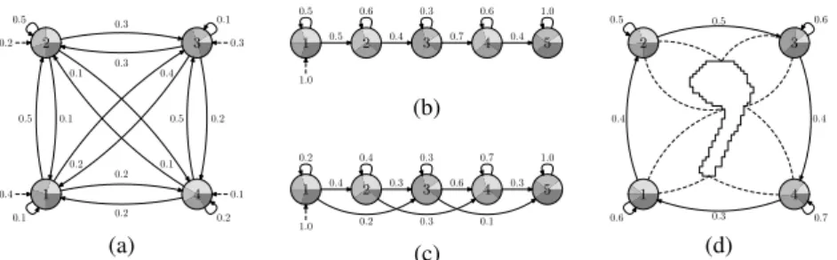
(3) 0.5 0.5. 0.6. 0.3. 0.6. 1.0. 0.1. 0.3. 2. 0.2. 3. 0.3. 0.5. 1. 0.5. 2. 0.4. 3. 0.7. 4. 0.4. 0.6. 0.5. 2. 5. 3. 0.3 0.1. 0.5. 0.4. 0.1. 1.0. 0.5. 0.2. (b). 0.2. 0.2. 0.1. 0.4. 0.4. 0.3. 0.7. 0.4. 1.0. 0.2 0.4 0.1. 1. 4 0.2. 0.1. 1. 0.2 1.0. (a). 0.4. 2 0.2. 0.3. 3 0.3. 0.6. 4 0.1. 0.3. 5. 1 0.6. (c). 4 0.3. 0.7. (d). Fig. 1. Examples of HMMs. An HMM state can emit any of four symbols according to the probability distribution represented by a pie chart. Probability distribution for initial states is represented by dotted arrows. (a) Ergodic topology with four states. (b) Linear left-to-right topology. (c) Bakis left-to-right topology. (d) Circular topology as proposed in [4]. Contours are segmented by associating a state to each segment. Ideally, each state is responsible for a single segment.. 2 Defining the Problem of Cyclic Strings with HMMs 2.1 Common Approaches One crucial aspect when applying HMMs is the definition of an adequate topology. Many works use ergodic topologies [5–7], which have some problems. The main is that it is possible to visit a state more than once without using self transitions (Fig. 1a). Ergodic models do not impose restrictions in the order of the strings of observations. When the string of observations is temporal or an order exists (as in shape contours), these topologies do not fully exploit the sequential or temporal information of the data and many states are used to explain multiple observations from different parts along the contour. This makes training and recognition a complex problem. From the previous observations, left-to-right topologies seem more suitable. These topologies do not allow to visit states that are to the left of the current one (Figs. 1b and 1c). In left-to-right models there is an initial state and a final state. This way, the sequence of states is forced to begin in the initial state and it never revisits a state once it lefts it. When a string of symbols is segmented, all the symbols of a segment are emitted by the same state, and consecutive segments are associated to consecutive states. Although these topologies usually have more states, their number of transitions is low, and consequently the overall complexity of the algorithms is reduced. In [4], a circular topology is proposed to model contours (Fig. 1d), which can be seen as a modification of the left-to-right topology, where the last emitting state is connected to the first. This topology eliminates the need for a starting point: the contour can be segmented by associating consecutive states to consecutive segments in the cyclic strings, but there is no assumption about which is the first or last segment (Fig. 1d); therefore, there is an analogy with left-to-right topologies. However, there is a problem that breaks this analogy: like in the case of ergodic models all the states can be reached from any state and we can finish in any of them. Therefore, the optimal path can contain non-consecutive repeated states and one state can be responsible of the emission of several non-consecutive segments of the contour. Besides, it is possible to have an optimal path that does not visit all the states at least once..

(4) (a). (b). Fig. 2. (a) Original shapes and their canonical versions using Fourier descriptors [9]. The same shapes compressed in the horizontal axis have different rotation and starting point. (b) Canonical version of an elephant with its trunk down and with its trunk raised using the method of least second moment of inertia [3].. Another approach is the election of a reference rotation and from it a starting point [3, 9]. The basic idea is that, after normalization, all shapes have a canonical version with a “standard” rotation and starting point, and thus, they can be compared as if their representations were linear. But invariance is only achieved for different rotations and starting points of the same shape. Different shapes (even similar ones) may differ substantially in their canonical orientation and starting point. Fig. 2a shows three perceptually similar figures whose canonical versions are significantly different in terms of orientation and starting point. This problem frequently appears in shapes whose basic ellipse is almost a circle. Besides, shapes of the same class with little differences can substantially alter the selection of the starting point. Fig. 2b shows two elephants, one with its trunk down and the other with its trunk raised, this fact and other little differences modify the canonical rotation of the method of least second moment of inertia, and with it, the selection of the starting point. 2.2 Cyclic Strings The most suitable solution for obtaining the invariance to the starting point is to use every possible starting point of the strings, i.e., using cyclic strings. A cyclic string can be seen as the set of strings obtained by cyclically shifting a conventional sequence. Let x = x1 . . . xm be a string from an alphabet Σ. The cyclic shift ρ(x) of a string x is defined as ρ(x1 . . . xm ) = x2 . . . xm x1 . Let ρk denote the composition of k cyclic shifts and let ρ0 denote the identity. Two strings x and x′ are cyclically equivalent if x = ρk (x′ ), for some k. The equivalence class of x is [x] = {ρk (x) : 0 ≤ k < m} and it is called a cyclic string. To achieve starting point invariance using cyclic strings we model the generation process as follows. An HMM generated a string that later suffered an unknown cyclic shift. That is, a model, λ, has generated a string, x = x1 x2 . . . xm , that has suffered the ′ transformation, ρk (x), for an unknown k ′ . We treat x as a cyclic string, [x], and we assume that all the cyclic shifts are equiprobable. Thus, the probability of [x] given a model λ is P ([x]|λ) =. m−1 X k=0. P (x|λ, k)P (k|λ) =. m−1 1 X P (ρk (x)|λ), m. (1). k=0. that is, we must compute the probability for every possible cyclic shift and add them..

(5) Similarly, finding the best cyclic shift and sequence of states amounts to compute P̂ ([x]|λ) =. 1 max P̂ (ρk (x)|λ) ∝ max P̂ (ρk (x)|λ). 0≤k≤m−1 m 0≤k≤m−1. (2). where P̂ is the Viterbi score for a string. Initially, we adopt P̂ as an estimation of the real probability because it is a very good approximation1.. 3 Cyclic Training To train HMMs cyclic strings we have to estimate the Markov model parameters that maximize the probability of the observed cyclic strings. That is, our objective is to maximize: (l). m −1 L Y 1 X P (ρk (x(l) )|λ), P ([x] |λ) = P (X|λ) = (l) m k=0 l=1 l=1 L Y. (l). (3). where X is a set of cyclic strings, X = {[x](1) , [x](2) , . . . , [x](L) }. We use an iterative procedure. First, we set some initial values for λ. Then, we obtain new values of these parameters in each iteration, using increasing transformations, applying the Baum-Eagon inequality [10, 11]. It is guaranteed that the new estimated values increase the value of the objective function and, therefore, its convergence. Let Σ = {v1 , v2 , . . . , vw }, be an alphabet (the set of observable events is discrete and finite). Let A = {aij } be the matrix of transition probabilities between states (1 ≤ i, j ≤ n, where n is the number of states) and let B = {bij } be the matrix Pn of observation probabilities (1 ≤ i ≤ n and 1 ≤ j ≤ w) [2]. As we know that j=0 aij = 1 for 0 ≤ i ≤ n and that (3) is a polynomial with respect to A, the new estimation, āij , can be obtained with the Baum-Eagon inequality [10, 11]. Applying logarithms and [10] to (3), we conclude that: Pm(l) −1 lk PL Pm(l) −1 (l) lk 1 αt (i)aij bj (ρk (xt+1 ))βt+1 (j) Pm(l) −1 t=0 k=0 l=1 k (x(l) )|λ) P (ρ k=0 , āij = Pm(l) −1 lk PL Pm(l) −1 lk 1 αt (i)βt+1 (j) Pm(l) −1 t=0 k=0 l=1 k (l) k=0. P (ρ (x. )|λ). (4) where αltk (i) and βtlk (j) are the forward and backward probabilities for the shifted string, ρk (x(l) ), and are defined similarly to those in [2]. Analogously, with Pbwi (vj ) (the probability of observing the symbol vj being in state i) and knowing that j=0 bi (vj ) = 1 for 1 ≤ i ≤ n and that (3) is a polynomial with respect to B (the matrix of observation probabilities [2]), we arrive at PL Pm(l) −1 Pm(l) −1 1 αltk (i)βtlk (i) Pm(l) −1 t=1 l=1 k=0 k (l) b̄i (vj ) =. PL Pm(l) −1 l=1. 1. k=0. k=0. P (ρ (x. Pm(l) −1 k=0. )|λ). 1 P (ρk (x(l) )|λ). (l). ∀ρk (xt )=vj. Pm(l) −1 t=1. αltk (i)βtlk (i). And it offers certain implementation advantages and reduction of computational time.. .. (5).

(6) A similar reasoning can be used for continuous models. This cyclic Baum-Welch (CBW) algorithm is an application of Expectation Maximization, and then, it needs a good initialization for λ. In the next section we propose a heuristic to solve this.. 4 A Heuristic for Selecting the Starting Point We will see in the experiments that the labelling of the training samples gives us an heuristic for obtaining a starting point that improves those in the literature (Section 2). We need to perform a preprocessing. For it we use cyclic DTW (CDTW) [1] that, apart from returning the cost (distance) of the cyclic alignment, can also return the corresponding cyclic shift of one of the strings for the alignment with the other string. Starting from a set of training samples, our aim is to choose an appropriate starting point for them. We select a representative (the centroid of the class using CDTW) and an arbitrary starting point for it. With the representative of each class and its starting point, we compute the CDTW for each one of the other members of the class and the representative, obtaining the cyclic shift of the alignment that defines a good starting point for each of them. Once we have an appropriate starting point for the training samples, we can train the model of each class as if the cyclic strings were ordinary strings. In a similar way, to classify a new sample, we begin by finding adequate starting points for it (one for each class). These starting points are computed by CDTW with the representative of each class. Thus, with this starting point for each class we can compute probabilities (or Viterbi scores) in a conventional way. Although, as we will see in the next section, this solution has worse results than the CBW algorithm, both training and recognition are much faster. Moreover this training can be used as a good initialization for the CBW algorithm.. 5 Experiments In order to assess the behaviour of the presented methods, we performed comparative experiments on a shape recognition task on publicly available databases: MPEG7 CEShape-1 corpus part B (MPEG7B) (1440 samples in 70 classes) [12], Silhouette corpus (1070 samples in 41 classes) [13], He-Kundu corpus (8 samples) [3] and Subset 1 corpus (7 classes of the MPEG7B corpus, 20 samples per class) [7]. The outer contours of the images were extracted as sequences of points. A random starting point in each sequence was also selected and 128 landmark points were sampled uniformly. As it is customary in the literature of HMMs and shape recognition we used the curvature shape descriptor. The evaluation was done with classification rates for different number of states (we train an HMM for each class): 10 to 120 in steps of 10. We only use a gaussian per state. The experiments of Section 5.1 were performed using cross validation. The ones of Section 5.2 were performed with a leaving-oneout approach for comparing with other results in the bibliography. In all of them, for classification, we use the Viterbi scores..

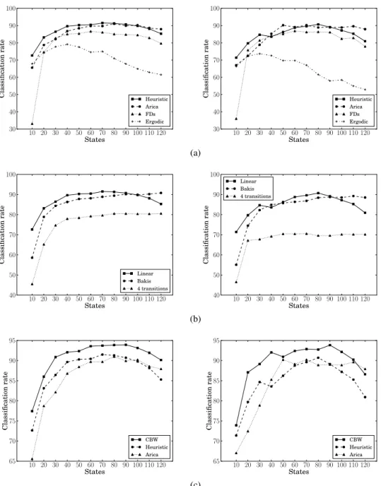
(7) 5.1 Invariance to the Starting Point, Left-to-right Topologies and Cyclic Approach In Section 2 several solutions to the starting point invariance problem are commented. We compare our heuristic (Section 4) with the circular topology [4], the election of the starting point using Fourier descriptors [3], and the ergodic topology [5–7]. In Fig. 3a the results of the comparison are shown, for MPEG7B and Silhouette corpora. The election of the starting point and the circular topology (especially the latter) happen to be the most competitive with respect to our heuristic while the ergodic topology obtains the worst results2 . In Section 2 we mentioned that left-to-right topologies are the most suitable for modelling strings. However, within these topologies, the linear topology seems to be the best for this purpose, because having more transitions increases the complexity of the model. Here we empirically prove this affirmation with a comparison between three left-to-right topologies: linear, Bakis and the one with four transitions per state. The last one is similar to Bakis but with another transition to the state three places from the current. The method used for training and classifying is our heuristic. The results are shown in Fig. 3b. As we can see the linear topology outperforms the others. We compare our cyclic approach, the CBW algorithm (Section 3) with our heuristic and the circular topology [4]. Cyclic training is initialized using the heuristic in a linear left-to-right topology. Comparative results are in Fig. 3c. We can observe that cases where CBW algorithm wins predominate. The best results that we obtain using CBW are 93.93% and 93.84% for the MPEG7B and Silhouette corpora. 5.2 More about the Ergodic Topology In Section 5.1 we experimentally saw that the ergodic topology does not offer good results. However, in the literature there are works [3, 5–7] where this topology is used. More specifically, in [5] experiments are performed with this topology. For training, the authors choose a number of states with BIC (Bayesian Inference Criterion) over a clustering of curvatures. The obtained results are good enough but their corpora have few samples and classes. They use a subset of the MPEG7B corpus of 6 classes with 10 samples per class (a subset of subset 1). They also use He-Kundu corpus for performing an experiment of invariance to the starting point achieving a classification rate of 100%. This way, they conclude that HMMs with an ergodic topology are enough for obtaining this invariance. In our opinion, this experiment is not enough for claiming that affirmation. For this corpus we also achieve a 100% with the CBW algorithm. In [6], a work of the same authors, another subset of MPEG7B is used (a subset of subset 1, with 12 samples per class). We call this corpus subset 2, as it is done in [7]. In this case, they use a canonical method for the election of the starting point. Instead of using BIC for obtaining the number of states, they use a fixed number of states. In [7], the authors, parting from the work of [5, 6], try to improve their results with a training based on GPD (Generalized probabilistic descent method). They also use the subset 2 and create a new one, subset 1. With subset 2 they obtain a classification rate of 97.63% ([6] obtains a 2. We will talk more about this topology in Section 5.2..

(8) 90. 90 Classification rate. 100. Classification rate. 100. 80 70 60 50 40 30. Heuristic Arica FDs Ergodic. 80 70 60 50 Heuristic Arica FDs Ergodic. 40 30. 10 20 30 40 50 60 70 80 90 100 110 120 States. 10 20 30 40 50 60 70 80 90 100 110 120 States. (a). 90. 90 Classification rate. 100. Classification rate. 100. 80 70 60 50 40. Linear Bakis 4 transitions. Linear Bakis 4 transitions. 80 70 60 50 40. 10 20 30 40 50 60 70 80 90 100 110 120 States. 10 20 30 40 50 60 70 80 90 100 110 120 States. 95. 95. 90. 90 Classification rate. Classification rate. (b). 85 80 75 70 65. CBW Heuristic Arica. 85 80 75 70 65. 10 20 30 40 50 60 70 80 90 100 110 120 States. CBW Heuristic Arica. 10 20 30 40 50 60 70 80 90 100 110 120 States. (c) Fig. 3. Classification rates (with corpora MPEG7B (left) and Silhouette (right)) for the comparison between: (a) The circular topology (Arica), the election of the starting point with Fourier descriptors (FDs), the ergodic topology (Ergodic) and our heuristic (Heuristic); (b) Different left-to-right topologies. Linear topology, Bakis topology and topology of four transitions. Our heuristic is used for training and classifying; and (c) cyclic Baum-Welch (CBW), our heuristic (Heuristic) and circular topology (Arica)..

(9) 98.8%). With subset 1 they obtain a 96.43%. With subset 1 and the CBW algorithm, we achieve a 99.28%, that even outperforms the classification rate of [6] with subset 2. None of the previous works show results with the entire MPEG7B corpus.. 6 Discussion In this work, we have argued and empirically proved that other proposals in the literature for obtaining the invariance to the starting point do not offer a suitable solution. We have formalized training and recognition for cyclic strings with Hidden Markov Models, formulating the corresponding Baum-Welch or Expectation Maximization algorithm. We have shown that this cyclic treatment is the current best solution for obtaining the starting point invariance.. References 1. Palazón-González, V., Marzal, A.: On the dynamic time warping of cyclic sequences for shape retrieval. Image and Vision Computing 30(12) (2012) 978–990 2. Rabiner, L.R.: A tutorial on hidden Markov models and selected applications in speech recognition. Proc IEEE 77(2) (1989) 3. He, Y., Kundu, A.: 2-D shape classification using hidden Markov model. IEEE Trans. Pattern Anal. Mach. Intell. 13(11) (November 1991) 1172–1184 4. Arica, N., Yarman-Vural, F.: A shape descriptor based on circular hidden Markov model. In: ICPR. Volume I. (2000) 924–927 5. Bicego, M., Murino, V.: Investigating hidden Markov models’ capabilities in 2D shape classification. IEEE Trans. Pattern Anal. Mach. Intell. 26(2) (2004) 281–286 6. Bicego, Murino, Figueiredo: Similarity-based classification of sequences using hidden Markov models. Pattern Recognition 37 (2004) 2281–2291 7. Thakoor, N., Gao, J., Jung, S.: Hidden Markov model-based weighted likelihood discriminant for 2-D shape classification. IEEE Trans. Image Processing 16(11) (November 2007) 2707–2719 8. Palazón, V., Marzal, A., Vilar, J.M.: Cyclic linear hidden Markov models for shape classification. In: PSIVT. (2007) 152–165 9. Bartolini, I., Ciaccia, P., Patella, M.: WARP: Accurate retrieval of shapes using phase of fourier descriptors and time warping distance. IEEE Trans. Pattern Anal. Mach. Intell. 27(1) (2005) 142–147 10. Baum, L.E., Eagon, J.A.: An inequality with applications to statistical estimation for probabilistic functions of Markov processes and to a model of ecology. Bull. Amer. Math. Soc. 73 (1967) 360–363 11. Levinson, S.E., Rabiner, L.R., Sondhi, M.M.: An introduction to the application of the theory of probabilistic functions of a Markov process to automatic speech recognition. The Bell System Technical Journal 62(4) (1983) 1035–1074 12. Latecki, L., Lakämper, R., Eckhardt, U.: Shape descriptors for non-rigid shapes with a single closed contour. In: CVPR, Los Alamitos, IEEE (June 13–15 2000) 424–429 13. Sharvit, D., Chan, J., Tek, H., Kimia, B.B.: Symmetry-based indexing of image databases. In: Workshop on Content-Based Access of Image and Video Libraries. (1998) 56–62.

(10)