Endogenous credit dynamics as source of business cycles in the EURACE model

Texto completo

(1)Endogenous credit dynamics as source of business cycles in the EURACE model Andrea Teglio, Marco Raberto, and Silvano Cincotti. Abstract The paper investigates the relationship between the amount of credit money in the economy and the variability of output and prices in the EURACE model. First we examine if the decision about dividends payment by the firms can affect this variability, then we adopt the policy measure of quantitative easing, that has been largely used by the Fed and the Bank of England during the recent crisis, in order to understand its effect on economic instability. Results show the emergence of endogenous business cycles which are mainly due to the interplay between the real economic activity and its financing through the credit market. In particular, the amplitude of the business cycles strongly raises when the fraction of earnings paid out by firms as dividends is higher, that is when firms are more constrained to borrow credit money to fund their activity.. Introduction The aim of this paper is to analyze the reasons of output and price variabilities in the EURACE economic environment. The issue is of primary importance, given that reducing macroeconomic volatility has numerous benefits. Lower volatility of inflation improves market functioning, makes economic planning easier, and reduces the resources devoted to hedging inflation risks. Lower volatility of output tends to imply more stable employment and a reduction in the extent of economic uncertainty confronting households and firms. Agent-based computational economics (ACE) has been characterized by a great deal of development in recent years (see Tesfatsion and Judd (2006) for a recent survey). There have been many studies regarding finance (see LeBaron (2006) for a reAndrea Teglio Departament d’Economia, Universitat Jaume I, Av. Sos Baynat, Castellón de la Plana, Spain, email: [email protected] Marco Raberto School of Science and Engineering, Reykjavik University, Menntavegur 1, 101 Reykjavik, Iceland e-mail: [email protected] Silvano Cincotti DIBE-CINEF, Università di Genova, Via Opera Pia 11a, 16145 Genova, Italy e-mail: [email protected]. 1.

(2) 2. Andrea Teglio, Marco Raberto, and Silvano Cincotti. view), while others have focused on labour and goods market (Tassier, 2001; Tesfatsion, 2001) or industrial organization (E. Kutschinski and Polani, 2003). However, only a few partial attempts have been made to model a multiple-market economy as a whole (Bruun, 1999; B. Sallans, 2003). In this respect, the EURACE simulator is certainly more complete, incorporating many crucial connections between the real economy and the credit and financial markets. In order to understand the recent crisis, and in general to understand the profound functioning of modern economies, we think it is not possible to ignore that connections any more. The aim of our paper is twofold. First we investigate if the decision about dividends payment by the firms can affect the variability of output and prices, and our results are clearly affirmative in this respect. Then we adopt the policy measure of quantitative easing, that has been largely used by the FED and the Bank of England during the recent crisis, in order to understand its effect on economic instability. In concrete terms, our experiments on the EURACE platform consist of different simulations for different parameter values. We take into consideration the effects of two critical parameters of the model. The first one, as said above, regards the financial management decision making of the firms, and corresponds to the fraction of net earnings paid by the firm to shareholders in form of dividends. The dividends decision impacts on many sectors of the model. In the financial market, for instance, agents beliefs on asset returns take into account corporate equity and expected cash flows, establishing an endogenous integration between the financial side and the real side of the economy. In particular, fundamentalist trading behavior is based on the difference between stock market capitalization and the book value of equity, therefore generating an interaction between the equity of the firm and the price of its asset in the financial market. Concerning the credit market, the dividends payment is strongly correlated with the loans request of the firm and consequently influences the amount of credit created by the commercial banks; as our results show in section 2, the credit amount proves to be decisive for its effects on the variability of output and prices. The second parameter of our study is a binary flag that activates the possibility for the central bank to buy treasure bills in the financial market, when a government asks for it. In practical terms, the central bank expands its balance sheet by purchasing government bonds. This form of monetary policy, widely adopted during the global financial and economic crisis of the years 2007-09, which is used to stimulate an economy where interest rates are close to zero, is called quantitative easing (QE). The creation of this new money is intended to seed the increase in the overall money supply through deposit multiplication by encouraging lending by these institutions and reducing the cost of borrowing, thereby stimulating the economy. Besides, quantitative easing is intended to help the funding of government budget deficit, by reducing the cost of debt as well as reducing the risk of debt rolling over. The paper is organized as follows. In section 1 it is given an overall description of the model with particular attention to the features that are relevant to this article. Section 2 presents the computational results of our study and a related discussion..

(3) Endogenous credit dynamics as source of business cycles in the EURACE model. 3. 1 The Model The EURACE model represents a fully integrated macroeconomy consisting of three economic spheres: the real sphere (consumption goods, investment goods, and labour market), the financial sphere (credit and financial markets), and the public sector (Government, Central Bank and Eurostat). Given the complexity of the underlying technological framework and given the considerable extension of the EURACE model, it is not possible to present within this paper an exhaustive explanation of the economic modelling choices, together with a related mathematical or algorithmic description. Consequently, we will limit our approach to a general qualitative explanation of the main key features of the model, treating in a concise way each different market, and giving prominence to those modelling aspects that attain to the argument of the specific analysis we are presenting in this paper. If the reader needs more details about the EURACE implementation, he will find a quite exhaustive summary in Eurace (2009). Moreover, when needed, we will cite specific EURACE deliverables. Some general information on EURACE can be found in Deissenberg et al. (2008). Both the modelling of agents behaviors and the modelling of markets protocols are empirically inspired by the real world. Agent decision processes follow the usual and realistic assumptions of agentbased economics about bounded rationality, limited information gathering and storage capacities, and limited computational capabilities of the economic agents; see e.g. Tesfatsion and Judd (2006) for a recent survey on this approach. These assumptions lead us to use simple heuristics to model the agents’ behaviour, derived from the management literature for firms, and from experimental and behavioural economics for consumers/investors (Deaton, 1992; Benartzi and Thaler, 1995). We also make use of experimental evidence from the psychological literature on decision making. For example, the modelling of households’ portfolio decisions on the financial market is based on Prospect Theory (see Tversky and Kahneman (1992)). The rules used by the agents are simple but not necessarily fixed. Their parameters can be subject to learning, and thus adapted to a changing economic environment. Here we can make a distinction between adaptive agents and learning agents: the first use simple stimulus-response behaviour to only adapt their response to their environment, while the last use a conscious effort to learn about the underlying structure of their environment. In the following more details are given regarding each market present in the model..

(4) 4. Andrea Teglio, Marco Raberto, and Silvano Cincotti. 1.1 Goods and labor markets For detailed information about the economic modelling choices characterizing the goods and the labor markets, see Eurace Project D7.1 (2007); Eurace Project D7.2 (2008). See also Dawid et al. (2008) and Dawid et al. (2009) for additional explanations and for some discussion and analysis of computational experiments directly involving the two markets. What follows is a qualitative description of the main aspects that are relevant to the paper. The goods markets are populated by IGFirms (investment goods firms) that sell capital goods to CGfirms (consumption goods firms), that produce the final consumption good. Stocks of firms product are kept in regional malls that sell them directly to households. A standard inventory rule is employed for managing the stock holding. Standard results from inventory theory suggest that the firm should choose its desired replenishment quantity for a mall according to its expectations on demand, calculated by means of a linear regression based on previous demands. Consumption good producers need physical capital and labor to produce. The production technology in the consumption goods sector is represented by a CobbDouglas type production function with complementarities between the quality of the investment good and the specific skills of employees for using that type of technology. Factor productivity is determined by the minimum of the average quality of physical capital and the average level of relevant specific skills of the workers. Capital and labor input is substitutable with a constant elasticity and we assume constant returns to scale. The monthly realized profit of a consumption goods producer is the difference of sales revenues achieved in the malls during the previous period and costs as well as investments (i.e. labor costs and capital good investments) borne for production in the current period. Wages for the full month are paid to all workers at the day when the firm updates its labor force. Investment goods are paid at the day when they are delivered. Consumption good producers employ a standard approach from the management literature, the so-called ‘break-even analysis’ to set their prices. The break-even formula determines at what point the change in sales becomes large enough to make a price reduction profitable and at what point the decrease in sales becomes small enough to justify a rise in the price. Basically, this managerial pricing rule corresponds to standard elasticity based pricing. Once a month households receive their income. Depending on the available cash, that is the current income from factor markets (i.e. labor income and dividends) plus assets carried over from the previous period, the household sets the budget which it will spend for consumption and consequently determines the remaining part which is saved. This decision is taken according to the buffer-stock saving theory (Deaton, 1992; Carroll, 2001). At the weekly visit to the mall in his region each consumer collects information about the range of goods provided and about the prices and inventories of the different goods. In the Marketing literature it is standard to describe individual consumption decisions using logit models. These models represent the stochastic influence of factors not explicitly modelled on consumption.We assume that a consumer’s de-.

(5) Endogenous credit dynamics as source of business cycles in the EURACE model. 5. cision about which good to buy is random, where purchasing probabilities are based on the values he attaches to the different choices he is aware of. Since in our setup there are no quality differences between consumer goods and we also do not take account of horizontal product differentiation, choice probabilities depend solely on prices. The labor market is governed by a matching procedure that relates directly workers looking for a job and firms looking for labor force. On the demand side, firms post vacancies with corresponding wage offers. On the supply side, unemployed workers or workers seeking for a better job, compare the wage offers with their actual reservation wages. Then the matching algorithm operates by means of ranking procedures on the side both of firms and households (see Eurace (2009) for more details). The algorithm might lead to rationing of firms on the labor market and therefore to deviations of actual output quantities from the planned quantities. In such a case the quantities delivered by the consumption good producer to the malls is reduced proportionally. This results in lower stock levels and therefore it generally increases the expected planned production quantities in the following period.. 1.2 Credit and financial markets For more detailed information on the financial market, see Eurace Project D6.1 (2007) and Eurace Project D6.2 (2008). Teglio et al. (2009) shows also economic results obtained by means of computational experiments in the financial market, mainly regarding the problem of the equity premium puzzle. The EURACE artificial financial market operates on a daily basis and is characterized by a clearing house mechanism for price formation which is based on the matching of the demand and supply curves. The trading activity regards both stock and government bonds, while market participants are households, firms and the governments. Both firms and governments may occasionally participate to the market as sellers, with the purpose to raise funds by the issue of new shares or governments bonds. Households provide most of the trading activity in the market, to which they participate both for saving and speculation opportunities. Household preferences are designed taking into account the psychological findings emerged in the framework of behavioral finance and in particular of prospect theory (Tversky and Kahneman, 1992). Households portfolio allocation is then modeled according to a preference structure based on a key prospect theory insight, i.e., the myopic loss aversion, which depends on the limited foresight capabilities characterizing humans when forming beliefs about financial returns (see Benartzi and Thaler (1995)). Firms finance investments and production plans preferably with internal resources. When these funds are not sufficient, firms rely on external financing, applying for loans to the banks in the Credit Market. The decision about firms loan request.

(6) 6. Andrea Teglio, Marco Raberto, and Silvano Cincotti. is taken by the bank to which the firm applies and depends on the total amount of risk the bank is exposed to, as increased by the risk generated by the additional loan. If a firm is credit-rationed in the Credit Market, then it has other possibilities of financing, i.e. issuing new equity on the financial market. Commercial banks have two roles: one consists in financing the production activities of the firms, operating under a Basel II-like regulatory regime. The other role is to ensure the functioning of the payment system among trading agents. Finally, firms and households deposit entirely their liquid assets in the banks. In the model banks are at the core of the system of payments: each transaction passes through the bank channel. Firms and households do not hold money as currency but under the form of bank deposits. Hence, the sum of payment accounts of bank’s clients is equal to bank’s deposits. As a consequence, every transaction (payment) between two non-financial agents translates into a transaction between two banks. At the end of every day, agents communicate the consistency of their liquid assets to their banks; then each bank can account for the net difference between inflows and outflows of money from and to the other banks and, if its reserves are negative, a compensating lending of last resort by the central bank is always granted. Thus, a sort of Deferred Net Settlement System has been implemented. The Central Bank has several function in the EURACE model. It helps banks by providing them with liquidity when they are in short supply. It has the role of monitoring the banking sector setting the maximum level of leverage each bank can afford. It decides the lowest level of the interest rate, which is a reference value for the banking sector. If the quantitative easing feature is active, the central bank expands its balance sheet by purchasing government bonds in the financial market. More details about the credit market of EURACE can be found in Eurace Project D5.1 (2007) and Eurace Project D5.2 (2008).. 2 Results Computational experiments has been performed in order to study the interplay between the supply of endogenous credit money and the performance of the economy, measured by the dynamics of the gross domestic product (GDP), the unemployment level, the dynamics of prices and the accumulation of physical capital in the economy. The dynamics of credit money is fully endogenous and depends on the supply of credit from the banking system, which is constrained by its equity base, and the demand of credit from firms in order to finance their production activity. Alternative dynamic paths for credit money have been produced by setting different firms’ dividend policies. The ratio d of net earnings that firms pay out as dividends has been exogenously set to four different values, namely, 0.6, 0.7, 0.8, and 0.9. It is clear that for higher values of d, firms’ investments and hiring of new labor force must be financed more by new loans than by retained earnings, thus determining a higher amount of credit money in the economy..

(7) Endogenous credit dynamics as source of business cycles in the EURACE model d QE no yes no 0.7 yes no 0.8 yes no 0.9 yes 0.6. 7. physical capital unemployment real GDP growth rate (%) rate (%) growth rate (%) -0.0015 14.9 0.13 0.0021 12.3 0.14 0.0005 13.2 0.11 0.0027 11.4 0.15 0.0038 13.6 0.15 0.0035 11.8 0.15 0.014 10.8 0.17 0.013 11.7 0.16. Table 1 Values report the ensemble averages over three different simulation runs of mean monthly rates. Each run is characterized by a different random seed. For each simulation run, mean monthly rates are computed over the entire simulation period, except for the first 12 months which have been considered as a transient and discarded.. Besides, the non conventional monetary policy practice called quantitative easing is considered, alongside the fiscal policy pursued by the Government. The central bank policy rate is kept fixed at low levels, however, if the quantitative easing (QE) policy is active, the central bank may buy government bonds directly on the market, thus increasing the overall amount of fiat money in the economy. Under quantitative easing, the government budget deficit is funded just by the issue and sale of bonds on the market. In this case, the intervention of the central bank is finalized to sustain bond prices and thus to facilitate the financing of government debt. If quantitative easing is not active, the government budget deficit in funded both by the issue of new bonds in the market and by an increase of tax rates. Each parameters’ setting is then characterized by one of the four values of d and by a binary variable which denotes whether the quantitative monetary policy is adopted. The total number of parameters settings then sums up to 8. In order to corroborate the significance of results, for each parameters setting, three different simulation runs have been considered, where each run is characterized by a proper. d QE no yes no 0.7 yes no 0.8 yes no 0.9 yes 0.6. Private sector money endowment price inflation wage inflation growth rate (%) rate (%) rate (%) -0.10 0.0019 0.19 -0.11 -0.0093 0.17 -0.09 -0.005 0.17 -0.11 -0.011 0.17 0.04 -0.08 0.18 0.089 0.030 0.18 0.35 0.12 0.28 0.33 0.10 0.27. Table 2 Values report the ensemble averages over three different simulation runs of mean monthly rates. Each run is characterized by a different random seed. For each simulation run, mean monthly rates are computed over the entire simulation period, except for the first 12 months which have been considered as a transient and discarded..

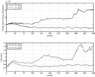
(8) 8. Andrea Teglio, Marco Raberto, and Silvano Cincotti. 6000 d = 0.6 d = 0.9. real GDP. 5000. 4000. 3000. 2000. 0. 36. 72. 108. 144. 180. 216. 252. 288. 324. 360. 216. 252. 288. 324. 360. months. Unemployment rate (%). 50 d = 0.6 d = 0.9. 40 30 20 10 0. 0. 36. 72. 108. 144. 180 months. Fig. 1 Results of a simulation path for the real gross domestic product (GDP) and the unemployment rate. Two values of d are considered, i.e., d = 0.6 (thick line) and d = 0.9 (thin line).. seed of the pseudorandom numbers generator. The same set of three random seeds has been employed for all parameters’ settings. The agents’ population is constituted by 1000 households, 10 consumption goods producing firms, 1 investment goods producing firms, 2 banks, 1 government and 1 central bank. The duration of each simulation is set to 360 months (30 years). Tables 1 and 2 report the simulation results for the main real and nominal variables of the economy, respectively, obtained with the 8 parameters’ settings considered. Figures 1 and 2 show two representative time paths for some of the variables considered. A clear and important empirical evidence that emerges from the path of GDP is that the EURACE model is able to exhibit endogenous business cycles. The main source of the observed business cycles is the strict relation between the real economic activity and its financing through the credit market, as it will be clear in what will follows. Here, we will describe the simulation results with respect to the different values of d considered. The qualitative considerations which emerge with respect to the value of d do not depend wether the quantitative easing policy is active or not. In particular, table 2 show that, as expected, an increase of the fraction d of firms’ earnings, which is payed out as dividends, increases the private sector money endowment. The effects on nominal variables is also evident from the Figure 2, where the simulation paths for the two extremes values of d, i.e., d = 0.6 and d = 0.9 are reported. The credit money supplied by the banking system is the source, together.

(9) Endogenous credit dynamics as source of business cycles in the EURACE model. 9. 4. Private sector money endowment. 4. x 10. d = 0.6 d = 0.9. 3. 2. 1. 0. 0. 36. 72. 108. 144. 180. 216. 252. 288. 324. 360. 216. 252. 288. 324. 360. months. 1.4 d = 0.6 d = 0.9. 1.3. Price level. 1.2 1.1 1 0.9 0.8 0.7 0. 36. 72. 108. 144. 180 months. Fig. 2 Results of a simulation path for the private sector money endowment and the price level. Two values of d are considered, i.e., d = 0.6 (thick line) and d = 0.9 (thin line).. with the fiat money supplied by the central bank, of the endowment of liquid resources held by both the private sector (households, firms and banks) and the public sector (government and central bank). An increase in the demand for credit by firms, if supplied by banks, then increases the amount of liquid resources in the economy. Table 2 also shows that higher inflation and wage rates are associated to higher values of d. Higher inflation rates for higher values of d should not be explained in this framework according to the quantity theory of money, due to the higher amount of liquidity in the economy. This because prices are not set by a fictitious Walrasian auctioneer at the cross between demand and supply, but are set by firms, based on their costs, which are labor costs, capital costs and debt financing costs. Higher credit money means higher debt and higher debt financing costs. Higher credit money induces also higher wage inflation, and thus again higher price inflation through the cost channel. The wage inflation can be explained by the labor market conditions, i.e., the level of unemployment, as it will be clear in the following. Table 1 presents the outcomes of the simulation concerning the real variables of the economy, i.e., unemployment level and rate of growth of physical capital and of real GDP. A clear indication emerges for a better macroeconomic performance, i.e., lower unemployment, and higher growth rate of real GDP and physical capital, related to higher levels of credit money in the economy. This indication is also corroborated by Figure 1, where two simulation paths for the real GDP and the un-.

(10) 10. Andrea Teglio, Marco Raberto, and Silvano Cincotti d QE no yes no 0.7 yes no 0.8 yes no 0.9 yes 0.6. first half second half (months: 12-180) (months: 181-360) -19.2 -18.7 -18.8 -22.0 -18.9 -16.6 -20.0 -21.0 -19.8 -26.1 -21.3 -22.9 -22.7 -31.1 -25.2 -37.5. Table 3 Values report the ensemble averages over three different simulation runs of the maximum percentage variability of the real GDP over a moving window of 60 month (5 years).. employment levels are reported for the two extreme values of d, i.e., d = 0.6 and d = 0.9. It is worth noting, however, that a higher credit money may increases the amplitude of the business cycle. This feature emerges from Figure 1 where both the real GDP and the unemployment level associated to d = 0.9 exhibit fluctuations which are far larger than the d = 0.6 case. In fact, a higher amount of credit money in the economy means higher levels of debt and leverage for firms. Firms bankruptcies due to insolvency (the equity goes negative) become more likely, and a firm bankruptcy causes mass layoffs and a sudden decrease in production. Besides, when a firm defaults on its debt, the lending bank suffers a reduction of its equity base, this in turn determine a reduction of the supply of credit and the production sector may face a credit rationing, thus triggering further bankruptcies, due to liquidity problems. Table 3, which reports the maximum percentage variability of real GDP in a moving time window of 60 months (5 years), confirms the graphic evidence of Figure 1. In particular, a further interesting pattern emerges if we divide the time period of the simulation into two parts, and the maximum is computed separately in each part. For values of d like 0.8 and 0.9, i.e., a parameters setting where firms are more constrained to borrow credit money to fund their activity, the percentage variability in the second part of the simulation time span is clearly higher. This fact can be explained by looking to the leverage of firms and number of bankruptcies which is higher in the second part, after the first part is characterized by increasing levels of firms debt and leverage to unsustainable levels. This empirical finding may somewhat resembles the relation between the so-called “great moderation" period of the 90s and the first part of the 00s for the world economy, and the so-called “great recession" observed during the last two years. The disaggregation of results with respect to the adoption or not of the quantitative easing monetary policy does not give a clear answer in the experiments considered about the goodness of a choice respect to another. The reason may be that in the setting considered, the government finances are usually sounds, so even if a quantitative easing policy is in principle adopted, it is applied just a few times..

(11) Endogenous credit dynamics as source of business cycles in the EURACE model. 11. 3 Concluding remarks In this paper, we investigated the relationship between the amount of credit money and the macroeconomic performance in the EURACE simulator. Given that the dynamics of credit money is determined endogenously in the system, different dynamic paths have been produced by setting different firms’ dividend policies. Results show the emergence of endogenous business cycles which are mainly due to the interplay between the real economic activity and its financing through the credit market. In particular, the amplitude of the business cycles strongly raises when the fraction of earnings paid out by firms as dividends is higher, that is when firms are more constrained to borrow credit money to fund their activity. This evidence can be explained by the fact that the level of firms leverage, defined as the debt-equity ratio, can be considered ad a proxy of the likelihood of bankruptcy, an event which causes mass layoffs and supply decrease. Finally, this results show the possibility to explain the emergence of business cycles based on the complex internal functioning of the economy, without any adhoc exogenous shocks. The adopted agent-based framework has been able to address this complexity, and these results reinforce the validity of the EURACE model and simulator for future research in economics.. Acknowledgements This work was carried out in conjunction with the EURACE project (EU IST FP6 STREP grant: 035086) which is a collaboration lead by S. Cincotti (Università di Genova), H Dawid (Universitaet Bielefeld), C. Deissenberg (Université de la Méditerranée), K. Erkan (TUBITAK-UEKAE National Research Institute of Electronics and Cryptology), M. Gallegati (Università Politecnica delle Marche), M. Holcombe (University of Sheffield), M. Marchesi (Università di Cagliari), C. Greenough (Science and Technology Facilities Council Rutherford Appleton Laboratory).. References B. Sallans, A. Pfister, A. K. G. D., 2003. Simulations and validation of an integrated markets model. Journal of Artificial Societies and Social Simulation 6 (4). Benartzi, S., Thaler, R. H., 1995. Myopic loss aversion and the equity premium puzzle. The Quarterly Journal of Economics 110 (1), 73–92. Bruun, C., 1999. Agent-based Keynesian economics: simulating a monetary production system bottom-up. University of Aaborg. Carroll, C. D., 2001. A theory of the consumption function, with and without liquidity constraints. Journal of Economic Perspectives 15 (3), 23–45..

(12) 12. Andrea Teglio, Marco Raberto, and Silvano Cincotti. Dawid, H., Gemkow, S., Harting, P., Kabus, K., Neugart, M., Wersching, K., 2008. Skills, innovation, and growth: An agent-based policy analysis. Journal of Economics and Statistics 228 (2+3), 251–275. Dawid, H., Gemkow, S., Harting, P., Neugart, M., 2009. On the effects of skill upgrading in the presence of spatial labor market frictions: an agent-based analysis of spatial policy design. Journal of Artificial Societies and Social Simulation 12 (4). Deaton, A., 1992. Household saving in ldcs: credit markets, insurance and welfare. The Scandinavian Journal of Economics 94 (2), 253–273. Deissenberg, C., van der Hoog, S., H., Dawid, 2008. Eurace: A massively parallel agent-based model of the european economy. Applied Mathematics and Computation 204, 541–552. E. Kutschinski, T. U., Polani, D., September 2003. Learning competitive pricing strategies by multi-agent reinforcement learning. J Econometrics 27 (11-12), 2207–2218. Eurace, 2009. Final activity report. http://www.eurace.org/. Eurace Project D5.1, 2007. Agent based models of goods, labour and credit markets. http://www.eurace.org. Eurace Project D5.2, 2008. Computational experiments of policy design on goods, labour and credit markets. http://www.eurace.org. Eurace Project D6.1, 2007. Agent based models of financial markets. http://www.eurace.org. Eurace Project D6.2, 2008. Computational experiments of policy design on financial markets. http://www.eurace.org. Eurace Project D7.1, 2007. Agent based models for skill dynamics and innovation. http://www.eurace.org. Eurace Project D7.2, 2008. Computational experiments of policy design on skill dynamics and innovation. http://www.eurace.org. LeBaron, B. D., 2006. Agent-based computational finance. Vol. 2 of Handbook of Computational Economics. North Holland. Tassier, T., 2001. Emerging small-world referral networks in evolutionary labor markets. IEEE Transaction of Evolutionary Computation 5 (5), 482–492. Teglio, A., Raberto, M., Cincotti, S., 2009. Explaining equity excess return by means of an agent-based financial market. Lecture Notes in Economics and Mathematical Systems. Springer Verlag, Ch. 12, pp. 145–156. Tesfatsion, L., 2001. Structure, behaviour, and market power in an evolutionary labour market with adaptive search. Journal of Economics Dynamics and Control 25, 419–457. Tesfatsion, L., Judd, K., 2006. Agent-Based Computational Economics. Vol. 2 of Handbook of Computational Economics. North Holland. Tversky, A., Kahneman, D., October 1992. Advances in prospect theory: cumulative representation of uncertainty. Journal of Risk and Uncertainty 5 (4), 297–323..

(13)