Nonparametric tests for homoscedasticity in randomized complete block designs

Texto completo

(1)Instituto Tecnológico y de Estudios Superiores de Monterrey Campus Monterrey. School of Engineering and Sciences. Nonparametric Tests for Homoscedasticity in Randomized Complete Block Designs. A thesis presented by. Pamela Lizeth Torres Núñez Submitted to the School of Engineering and Sciences in partial fulfillment of the requirements for the degree of Master of Science. in Manufacturing Systems Monterrey, Nuevo León, May 31st , 2019.

(2)

(3)

(4) iii. @2019 by Pamela Lizeth Torres Núñez All rights reserved.

(5) iv. Dedication I want to dedicate this work to my parents Mr. Benjamin and Mrs. Josefina, that always have been my force to go ahead in each step that I move on, they are my model, they teach me that every e↵ort will be recognized but, first I need to do all that I can do, and when I cannot, the next thing is looking for the inspiration that I need and continue with the goal that put me there in the first instance. From them I learned the humility to accept when I need help, and recognize that I was wrong. To my siblings, Benjamin, Norma, Jessica, Carlos and Jorge, they have been an excellent model to me that inspires me. To my nieces, Salma, Alexa, Sofia, and Mabel, to demonstrate them that all the goals can be possible if they put all the discipline, attitude and if they believe in themselves. Finally, to these people that have a goal that they know that the only limit to reach them are themselves..

(6) v. Acknowledgments Another goal is to achieve in my life, but, this could not be possible if I did not have my support network. For this reason, I would like to express all my gratitude to all the people that always have been on my side in this way. Thanks to my parents for all their love, patience, and preoccupation that always received from them. To my siblings, Benjamin, Norma, Jessica, Carlos, and Jorge, for always give me them support, and the confidence to know that if the things do not give me the result that I expect, I will always have my family there to share all my achievements but, also the failures that I could have on the way. For still believing in me. To my advisers for their guide, for demanding me more of what I thought I could give, for their help in all my doubts. To my friends whose always demonstrated me that they were here for me if I need it, that shared with me all these long nights of work, stress, laughs and great moments that I will save on my memory and heart. A special acknowledgment to the Tecnologico de Monterrey and CONACyT for allow me to be part of this program, for all the sources provided and the supports on tuition and living place. To God, to o↵er me all that I required to follow my goals, to give me the beautiful people that I have on my side.. Thanks..

(7) vi. Nonparametric Tests for Homoscedasticity in Randomized Complete Block Designs By Pamela Lizeth Torres Núñez. Abstract Variance assessment is a key component in robust design, process improvement, and reliability analysis, among other practical venues. However, most statistical development in nonparametric statistics has been focused on the problem of location changes, whereas the development of tests for homoscedasticity has been scarce, limited, in most cases, to one-factor analysis. By considering a blocking element, in the sense of Friedman, more power can be obtained by extending the approach to be used with linear rank transformations sensitive to scale changes. In this research, a total of 96 di↵erent new linear rank tests for homoscedasticity have been created, and their robustness and power evaluated through extensive Monte Carlo simulations. 36 of these tests showed to be either distribution robust or distribution free. 5 approaches of within the remaining tests acted consistently with high power over scale changes, and only 3 (Fligner-Killeen, squared ranks, and TalwarGentle, the three are aligned with the overall median) of these tests remained powerful when dealing with scale and location changes. Based on their performance, and easy of use, practitioners and researchers might find the results and recommendations of this work compelling and useful for their practice of data analysis when dealing with nuisance factors in the form of blocks..

(8) Contents 1 Introduction 1.1 Motivation . . . . . . 1.2 Problem statement . 1.3 Research questions . 1.4 Research hypotheses 1.5 Scope and limitations 1.6 Main contributions .. . . . . . .. . . . . . .. . . . . . .. . . . . . .. . . . . . .. . . . . . .. . . . . . .. . . . . . .. . . . . . .. . . . . . .. . . . . . .. . . . . . .. . . . . . .. 2 Background and literature review 2.1 Background . . . . . . . . . . . . . . . . . . 2.1.1 Design and analysis of experiments . 2.1.2 Analysis of variance: one way . . . . 2.1.3 Analysis with fixed e↵ects model . . 2.1.4 Model Adequacy . . . . . . . . . . . 2.1.5 Randomized Complete Block Design 2.2 Literature Review . . . . . . . . . . . . . . . 2.2.1 Previous works . . . . . . . . . . . .. . . . . . .. . . . . . . . .. . . . . . .. . . . . . . . .. 3 Methodology 3.1 Mathematical Framework . . . . . . . . . . . . 3.1.1 Assumptions . . . . . . . . . . . . . . 3.1.2 Friedman’s Test statistic . . . . . . . . . 3.1.3 Friedman’s hypothesis and reject region . 3.2 Methodology . . . . . . . . . . . . . . . . . . . 3.2.1 Select scoring type and alignment . . . . 3.2.2 Test statistics . . . . . . . . . . . . . . . 3.2.3 Hypothesis . . . . . . . . . . . . . . . . . 3.2.4 Summary of the proposed procedure . . vii. . . . . . .. . . . . . . . .. . . . . . . . . .. . . . . . .. . . . . . . . .. . . . . . . . . .. . . . . . .. . . . . . . . .. . . . . . . . . .. . . . . . .. . . . . . . . .. . . . . . . . . .. . . . . . .. . . . . . . . .. . . . . . . . . .. . . . . . .. . . . . . . . .. . . . . . . . . .. . . . . . .. . . . . . . . .. . . . . . . . . .. . . . . . .. 1 3 4 4 5 6 7. . . . . . . . .. 9 9 9 11 12 14 15 18 18. . . . . . . . . .. 23 23 24 24 24 25 25 27 28 29.

(9) viii. 4 Simulation Desing and Results 4.1 Simulation Design . . . . . . . . 4.1.1 Generate a scenario . . . 4.2 Results . . . . . . . . . . . . . . 4.2.1 Symmetric Distributions 4.2.2 Skewed Distributions . . 4.3 Discussion . . . . . . . . . . . .. CONTENTS. . . . . . .. . . . . . .. . . . . . .. . . . . . .. . . . . . .. . . . . . .. . . . . . .. . . . . . .. . . . . . .. . . . . . .. . . . . . .. . . . . . .. . . . . . .. . . . . . .. . . . . . .. . . . . . .. . . . . . .. 31 31 34 35 35 40 54. 5 Example. 63. 6 Conclusions. 67.

(10) List of Figures 4.1. 4.2. 4.3. A comparison between the average power of the test statistics 2F , 2K , Fone , and Ftwo dealing with di↵erent number of replicates (2,10,20,50, and 100). . . . . . . . . . . . . . . . . . Comparison between the average power of the tests for homoscedasticity with the Fone test statistic, dealing with di↵erent number of replicates (2, 5, 10, 20, and 100) when there are no changes in the location for 2 and 4 treatment and 2,4, and 8 blocks. . . . . . . . . . . . . . . . . . . . . . . . . . . . . . . Comparison between the average power of the tests for homoscedasticity with the Fone test statistic, dealing with di↵erent number of replicates (2, 5, 10, 20, and 100) when there are changes in the location [(-1 1), (-2 2), (-3 3)], and [(-1 -1 1 1), (-2 -2 2 2), (-3 -3 3 3)] for 2 and 4 treatment and 2,4, and 8 blocks. Treatment standard deviations are (1 2), (1 3), (1 4)] and [(1 1 2 2), (1 1 3 3), (1 1 4 4)] for 2 and 4 treatments respectively . . . . . . . . . . . . . . . . . . . . . . . . . . . .. ix. 56. 57. 59.

(11) x. LIST OF FIGURES.

(12) List of Tables 2.1 2.2 2.3 2.4. An experiment with one factor. . . . . . . . . . . . . . . . . . ANOVA in fixed e↵ects model - one factor. . . . . . . . . . . . Randomized complete block design Conover (1999). . . . . . . ANOVA in a randomized complete block design (see Montgomery). . . . . . . . . . . . . . . . . . . . . . . . . . . . . . .. 11 14 16. 3.1 3.2 3.3. Scores. . . . . . . . . . . . . . . . . . . . . . . . . . . . . . . . Alignment. . . . . . . . . . . . . . . . . . . . . . . . . . . . . . Tests statistics with the combination of scores and alignments.. 25 26 26. 4.1. Initial assessment. Type I error probabilities over two 2 statistics. Robust test are highlighted. . . . . . . . . . . . . . 32 Performance with the Normal distribution of di↵erent test homoscedasticity using statistics 2F , 2K , Fone , and Ftwo with 2,4, and 8 blocks when dealing with no changes in the mean of 2 and 4 treatments [(0 0) and (0 0 0 0), respectively], and changes in mean between 2 and 4 treatments [(-3 3) and (-3 -3 3 3), respectively]. All mean changes are measured in standard deviations of the null distribution. Treatment standard deviations are (1 1) and (1 1 1 1) for 2 and 4 treatments respectively. 36 Performance with the Normal distribution of di↵erent test homoscedasticity using statistics 2F , 2K , Fone , and Ftwo with 2,4, and 8 blocks when dealing with no changes in the mean of 2 and 4 treatments [(0 0) and (0 0 0 0), respectively], and changes in mean between 2 and 4 treatments [(-3 3) and (-3 -3 3 3), respectively]. All mean changes are measured in standard deviations of the null distribution. Treatment standard deviations are [(1 2), (1 3), and (1 4)] and [(1 1 2 2), (1 1 3 3), and (1 1 4 4)] for 2 and 4 treatments respectively. . . . . . . . 38. 4.2. 4.3. xi. 18.

(13) xii. LIST OF TABLES. 4.4. 4.5. 4.6. 4.7. Performance with the Double exponential distribution of different test homoscedasticity using statistics 2F , 2K , Fone , and Ftwo with 2,4, and 8 blocks when dealing with no changes in the mean of 2 and 4 treatments [(0 0) and (0 0 0 0), respectively], and changes in mean between 2 and 4 treatments [(-3 3) and (-3 -3 3 3), respectively]. All mean changes are measured in standard deviations of the null distribution. Treatment standard deviations are (1 1) and (1 1 1 1) for 2 and 4 treatments respectively. . . . . . . . . . . . . . . . . . . . . . . . . . . . . Performance with the Double exponential distribution of different test homoscedasticity using statistics 2F , 2K , Fone , and Ftwo with 2,4, and 8 blocks when dealing with no changes in the mean of 2 and 4 treatments [(0 0) and (0 0 0 0), respectively], and changes in mean between 2 and 4 treatments [(-3 3) and (-3 -3 3 3), respectively]. All mean changes are measured in standard deviations of the null distribution. Treatment standard deviations are [(1 2), (1 3), and (1 4)] and [(1 1 2 2), (1 1 3 3), and (1 1 4 4)] for 2 and 4 treatments respectively. . . . Performance with the Normal squared distribution of di↵erent test homoscedasticity using statistics 2F , 2K , Fone , and Ftwo with 2,4, and 8 blocks when dealing with no changes in the mean of 2 and 4 treatments [(0 0) and (0 0 0 0), respectively], and changes in mean between 2 and 4 treatments [(-3 3) and (-3 -3 3 3), respectively]. All mean changes are measured in standard deviations of the null distribution. Treatment standard deviations are (1 1) and (1 1 1 1) for 2 and 4 treatments respectively. . . . . . . . . . . . . . . . . . . . . . . . . . . . . Performance with the Normal squared distribution of di↵erent test homoscedasticity using statistics 2F , 2K , Fone , and Ftwo with 2,4, and 8 blocks when dealing with no changes in the mean of 2 and 4 treatments [(0 0) and (0 0 0 0), respectively], and changes in mean between 2 and 4 treatments [(-3 3) and (-3 -3 3 3), respectively]. All mean changes are measured in standard deviations of the null distribution. Treatment standard deviations are [(1 2), (1 3), and (1 4)] and [(1 1 2 2), (1 1 3 3), and (1 1 4 4)] for 2 and 4 treatments respectively. . . .. 39. 41. 42. 44.

(14) LIST OF TABLES. Performance with the Double exponential squared distribution of di↵erent test homoscedasticity using statistics 2F , 2K , Fone , and Ftwo with 2,4, and 8 blocks when dealing with no changes in the mean of 2 and 4 treatments [(0 0) and (0 0 0 0), respectively], and changes in mean between 2 and 4 treatments [(-3 3) and (-3 -3 3 3), respectively]. All mean changes are measured in standard deviations of the null distribution. Treatment standard deviations are (1 1) and (1 1 1 1) for 2 and 4 treatments respectively. . . . . . . . . . . . . . . . . . . 4.9 Performance with the Double exponential squared distribution of di↵erent test homoscedasticity using statistics 2F , 2K , Fone , and Ftwo with 2,4, and 8 blocks when dealing with no changes in the mean of 2 and 4 treatments [(0 0) and (0 0 0 0), respectively], and changes in mean between 2 and 4 treatments [(-3 3) and (-3 -3 3 3), respectively]. All mean changes are measured in standard deviations of the null distribution. Treatment standard deviations are [(1 2), (1 3), and (1 4)] and [(1 1 2 2), (1 1 3 3), and (1 1 4 4)] for 2 and 4 treatments respectively. . . . . . . . . . . . . . . . . . . . . . . . . . . . . 4.10 Performance with the Lognormal distribution of di↵erent test homoscedasticity using statistics 2F , 2K , Fone , and Ftwo with 2,4, and 8 blocks when dealing with no changes in the mean of 2 and 4 treatments [(0 0) and (0 0 0 0), respectively], and changes in mean between 2 and 4 treatments [(-3 3) and (-3 -3 3 3), respectively]. All mean changes are measured in standard deviations of the null distribution. Treatment standard deviations are (1 1) and (1 1 1 1) for 2 and 4 treatments respectively. 4.11 Performance with the Lognormal distribution of di↵erent test homoscedasticity using statistics 2F , 2K , Fone , and Ftwo with 2,4, and 8 blocks when dealing with no changes in the mean of 2 and 4 treatments [(0 0) and (0 0 0 0), respectively], and changes in mean between 2 and 4 treatments [(-3 3) and (-3 -3 3 3), respectively]. All mean changes are measured in standard deviations of the null distribution. Treatment standard deviations are [(1 2), (1 3), and (1 4)] and [(1 1 2 2), (1 1 3 3), and (1 1 4 4)] for 2 and 4 treatments respectively. . . . . . . .. xiii. 4.8. 45. 47. 48. 50.

(15) xiv. LIST OF TABLES. 4.12 Performance with the Gamma distribution of di↵erent test homoscedasticity using statistics 2F , 2K , Fone , and Ftwo with 2,4, and 8 blocks when dealing with no changes in the mean of 2 and 4 treatments [(0 0) and (0 0 0 0), respectively], and changes in mean between 2 and 4 treatments [(-3 3) and (-3 -3 3 3), respectively]. All mean changes are measured in standard deviations of the null distribution. Treatment standard deviations are (1 1) and (1 1 1 1) for 2 and 4 treatments respectively. . .. 51. 4.13 Performance with the Gamma distribution of di↵erent test homoscedasticity using statistics 2F , 2K , Fone , and Ftwo with 2,4, and 8 blocks when dealing with no changes in the mean of 2 and 4 treatments [(0 0) and (0 0 0 0), respectively], and changes in mean between 2 and 4 treatments [(-3 3) and (-3 -3 3 3), respectively]. All mean changes are measured in standard deviations of the null distribution. Treatment standard deviations are [(1 2), (1 3), and (1 4)] and [(1 1 2 2), (1 1 3 3), and (1 1 4 4)] for 2 and 4 treatments respectively. . . . . . . .. 53. 4.14 Performance with the Weibull distribution of di↵erent test homoscedasticity using statistics 2F , 2K , Fone , and Ftwo with 2,4, and 8 blocks when dealing with no changes in the mean of 2 and 4 treatments [(0 0) and (0 0 0 0), respectively], and changes in mean between 2 and 4 treatments [(-3 3) and (-3 -3 3 3), respectively]. All mean changes are measured in standard deviations of the null distribution. Treatment standard deviations are (1 1) and (1 1 1 1) for 2 and 4 treatments respectively. 60 4.15 Weibull distribution - null hypothesis. . . . . . . . . . . . . . .. 60. 4.16 Performance with the Weibull distribution of di↵erent test homoscedasticity using statistics 2F , 2K , Fone , and Ftwo with 2,4, and 8 blocks when dealing with no changes in the mean of 2 and 4 treatments [(0 0) and (0 0 0 0), respectively], and changes in mean between 2 and 4 treatments [(-3 3) and (-3 -3 3 3), respectively]. All mean changes are measured in standard deviations of the null distribution. Treatment standard deviations are [(1 2), (1 3), and (1 4)] and [(1 1 2 2), (1 1 3 3), and (1 1 4 4)] for 2 and 4 treatments respectively. . . . . . . .. 61.

(16) LIST OF TABLES. 5.1 5.2. 5.3. Survival times of the animals in a factorial experiment. Example of agents. . . . . . . . . . . . . . . . . . . . . . . . . . . Obtain the individual scores for each test, using the overall median alignment over the residuals of the survival time in the four groups of animals (treatments), and the three di↵erent toxic agents (block). . . . . . . . . . . . . . . . . . . . . . . . Summary of results for the tests TG, SR, and FK aligned with the overall median. . . . . . . . . . . . . . . . . . . . . . . . .. xv. 63. 64 65.

(17) xvi. LIST OF TABLES.

(18) Chapter 1. Introduction. 1. Chapter 1 Introduction Research areas in manufacturing are involved in the execution of experiments in a specific process or product to discover or validate the behavior of that process or product when natural or artificial variations are included. As the majority of these variations are controlled (artificial changes), the observed variables can be tested (Montgomery, 2008). In the manufacturing industry, the analysis of these variations is conducted within the framework of Design and Analysis of Experiments (DOE), where the study of di↵erences is used as a base to develop robust products and processes, as well as process capability and reliability improvements. Traditionally, this analysis is carried following parametric approaches where the robustness of the ANOVA F test to nonnormal data had analyzed location changes practical and reliable. However, tests for scale changes are more sensitive to the normality assumption, and practitioners have to rely more on di↵erent statistical approaches, such as the use of nonparametric methods. However, the development of nonparametric procedures to deal with changes in scale has been scarce, and limited in most cases to one factor analysis. A gap in data analysis to address these issues, as is the case of treatment comparisons when nuisance factors are involved in the form of a block, requires further development. This research, is an attempt to fill this gap. A major intention of applying a DOE in a process is to improve its performance, i.e., to reduce cycle times, cost, defects and variability. Through treatment analysis, experiments are conducted to demonstrate a cause-e↵ect relation between one or more explanatory variable (process inputs), and a response variable (a quality characteristic). However, the presence of nuisance factors might increase the experimental error, intensifying the difficulty of the analysis and sometimes reducing the power to detect treatment changes. To.

(19) Chapter 1. Introduction. 2. deal with nuisance factors, researchers had created designs like Randomized Complete Block Design (RCBD), where nuisance factors are controlled in the form of blocks. This reduces the experimental error, making the analysis suitable to detect subtle changes between treatments, with high power. Also, as blocks are designed to be heterogeneous between themselves, practitioners gain the ability to generalize their conclusions, as their discoveries hold for the plurality of conditions defined by each block analyzed (see Kutner et al., 2005, for details). To determine if a variation is acceptable or not, acceptance interval are determined, and tools and equipment are developed to perform a test to a process. Several tests are used to measure the variability, one of the most popular between statisticians is the analysis of variance, which allows practitioners to determine if di↵erences exist (or not) between two or more samples by comparing their means using di↵erent treatments. (Angel Gutierrez, 1996). This method requires few assumptions: (a) The error variables are mutually independent within each block. (b) The error terms are normally distributed. (c) The error terms have constant variance (Kutner et al., 2005). In this research, we are dealing with the problem when the last two assumptions are not accomplished. First, the assumption that the data come from a normal distribution facilitates the selection of statistical tools such as ANOVA for the processing of the information. This generates errors of the variation in the distributions, comparing them with the normal ones. There are cases in which it is difficult to obtain the distribution, in these situations nonparametric statistical methods are used, that perform the analysis of data in the variables whose distribution is not specific. Nonparametric procedures are applicable in many cases where normal theory procedures cannot be utilized. The nonparametric methods require just the ranks of the observations (Hollander et al., 2013). The disadvantage of these methods is their inaccuracy. There are several critical factors in the implementation of sampling to properly analyze data; one of them is the distribution function (Conover, 1999). Another factor is the sample size due to the restrictions of many tests to e↵ectively work with a reliable sample science study. Second, the assumption of constant variance, di↵erent processes, and products made in a company may seem the same, but in reality, they are not. Variations in quality characteristics can be very significant. Variables such.

(20) Chapter 1. Introduction. 3. as time, resistance and weight determine acceptable processes or products when a specification interval is accomplished. The quality of a product is measured by its variation concerning the desired and depends on the existing variation in quality characteristics (Angel Gutierrez, 1996). Therefore, this study focuses on addressing these problems by developing and evaluating the equality of variances using nonparametric methods when the distribution is unknown. To evaluate the performance several distributions were used. These are normal, double-exponential (Laplace), in the case of the symmetric distributions; the distributions normal-square (chi-squared with one degree of freedom), Double-exponential-square, log-normal, Gamma and Weibull for the skewed distributions. Each distribution was evaluated over di↵erent scenarios that are generated by changing the sample size (2 and 4), the standard deviation, the e↵ect of the treatment, the number of replicates per cell, and the size of the block (2, 4, and 8). One more variation considered was the statistic to test the hypothesis, four statistics were used over di↵erent linear rank transformation as a way to create new statistics; two considering the 2 distribution, one of them is which is used in Friedman’s test (Conover, 1999), the other from the test of Kruskal Wallis (Hollander et al., 2013) and two for the Snedecor’s F. 1.1. Motivation. In a manufacturing process of a company, there are three di↵erent processes for cable coating that are carried out in three shifts per day. You want to know if there is a di↵erence in the variability of the process. To address this type of situations, we need to use a particular kind of designs as Randomized Complete Block Design (RCBD), in which the shift is a nuisance factor that can be treated as a block to reduce the noise and improve the power; the treatments are the types of coating. This type of applications is what motivates this study, to establish methods where the presence of blocks is detected, and we want to know if there is a significant change in variability between treatments when nuisance factors in the form of block exist..

(21) Chapter 1. Introduction. 1.2. 4. Problem statement. This research focuses on the problem of the development nonparametric statistical methods to study the e↵ect of treatments of an experimental study on the variance of a variable of interest when dealing with completely randomized experimental designs with replications. The principal restrictions in these cases are the nonnormality of the residuals.. 1.3. Research questions. 1. Which tests statistics are distribution robust? 2. Which tests for homoscedasticity are considered robust when there is also a change in the mean? 3. Which tests are considered sensitive for both location and scale changes? 4. In regard to the power within robust test for location: (a) Which test provides the most overall power? (b) Which test has the biggest power when the distribution is symmetric? (c) Which test has the biggest power when the distribution is asymmetric? (d) Which test has more power when dealing with the di↵erent number of replicates? (e) Which test has more power when dealing with relatively di↵erent numbers of treatments? (f) Which test has more power when dealing with relatively di↵erent numbers of blocks? 5. In regard to the power within tests sensitive to scale and location changes: (a) Which test provides the most overall power? (b) Which test has the biggest power when the distribution is symmetric?.

(22) Chapter 1. Introduction. 5. (c) Which test has the biggest power when the distribution is asymmetric? (d) Which test has more power when dealing with the di↵erent number of replicates? (e) Which test has more power when dealing with relatively di↵erent numbers of treatments? (f) Which test has more power when dealing with relatively di↵erent numbers of blocks?. 1.4. Research hypotheses. 1. At least one test is distribution robust or distribution free, where a test is considered robust if the probability of a type 1 error of 0.05 is not bigger than 0.1. 2. At least one test is robust to changes in location, where a test is considered robust if the probability of a type 1 error of 0.05 is not bigger than 0.1. 3. At least one test is sensitive for both location and scale changes. 4. In regard of the power within robust test for location: (a) At least one test has the most overall power. (b) At least one test has the most power when the distribution is symmetric. (c) At least one test has the most power when the distribution is asymmetric. (d) At least one test has the most more power when dealing with different number of replicates. (e) At least one test has the most power when dealing with relatively di↵erent numbers of treatments. (f) At least one test has the most power when dealing with relatively di↵erent numbers of blocks. 5. In regard of the power within tests sensitive to scale and location changes:.

(23) Chapter 1. Introduction. 6. (a) At least one test has the most overall power. (b) At least one test has the most power when the distribution is symmetric. (c) At least one test has the most power when the distribution is asymmetric. (d) At least one test has the most more power when dealing with different number of replicates. (e) At least one test has the most power when dealing with relatively di↵erent numbers of treatments. (f) At least one test has the most power when dealing with relatively di↵erent numbers of blocks.. 1.5. Scope and limitations. The scope of this research is limited to the analysis of linear rank statistics. As analytical solutions are hard to obtain (no known analytical solution is known for limited sample behaviour) the performance of each statistics is limited to Monte Carlo simulations over the following combination factors: • The number of replicates per cell could be 2,5,10,20,50, and 100. • The distributions selected were normal, normal-squared, double exponential, double-exponential squared, lognormal, gamma and Weibull. • The number of treatments compared were 2 and 4. • The block size could be 2,4, or 8. • The e↵ect of the treatment varies (this will be shown later). • Change in standard deviation (this will be shown later). Due to a large number of scenario analyzed, the number of simulations was limited to 1000..

(24) Chapter 1. Introduction. 1.6. 7. Main contributions. New nonparametric statistical tests for homoscedasticity in RCBD were created that are capable of dealing with symmetrical and skewed distributions with competitive power. Performance of each test was analyzed with a different distribution, sample size, replicate size, and block size..

(25) Chapter 1. Introduction. 8.

(26) Chapter 2. Background and literature review. 9. Chapter 2 Background and literature review 2.1 2.1.1. Background Design and analysis of experiments. An experiment can be defined as a test where a practitioner makes deliberate changes into a variable of a process or product to observe and analyze the change reasons in its response. The experimentation is a key factor for the development of new knowledge, processes, and products. One of the main objectives when designing a product or process is to develop a robustness, that is, a product or process that is less a↵ected by external sources of variation. In general, the objectives of an experiment could be: (a) To determine the variables that have a significant influence on the response. (b) To determine the necessary levels of a independent variables that could keep the response in a nominal value. (c) To determine how to modify a set of independent variables to reduce the variability of a response. (d) To determine a level of the independent variables that could potentially reduce the e↵ect of external and uncontrolled variables. There are three basic principles in the design of an experiment: 1. Replicates. A replicate or an experimental unit, are the times that an experiment is carried out under identical conditions. The replicates have.

(27) Chapter 2. Background and literature review. 10. essential properties. First, it makes possible the calculation of the experimental error; which is used to determine if the observed di↵erences are or aren’t statistically significant. Second, the use of replicates allows the experimenter to reduce the uncertainty of an estimation. 2. Randomization. By randomization, it is understood that the assignment of a treatment to an experimental unit was determined randomly. The use of randomization is a requirement for many statistical procedures. Randomization helps to reduce the minimum the influence of extraneous factors that are not under control. Also, it provides a solid ground when making inferences about cause and e↵ect relationships Kutner et al. (2005). 3. Blocking. This technique is used to improve the precision between the variables (factors) of interest. It reduces the variability occasioned by the nuisance factors. The nuisance factors are those who can influence the response, but there is not a specific interest. In this experiment, the experimental material is grouped into homogeneous subgroups called blocks, and separate tests are conducted in each block. Ideal blocks are constructed so that the experimental units are homogeneous within the blocks, but heterogeneous between them. Other benefits of this technique is that the validity of the conclusions obtained is increase with this method. Randomization within blocks provides additional protection against the unknown cause of variability. Hypothesis test In statistics, procedures used to make inference of a population from the analysis of data from an experiment are called hypothesis test and confidence intervals. A statistical hypothesis is an affirmation that is made about the parameters of a distribution. This reflects some supposition about a problem or a situation. For example, if the situation is to prove if two groups of students A and B have the same average grades, this hypothesis can be enunciated as H 0 : µ 1 = µ2 . H1 : µ1 6= µ2 ..

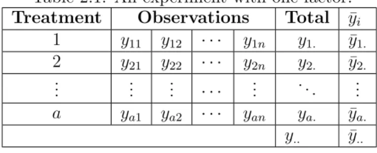
(28) Chapter 2. Background and literature review. 11. Table 2.1: An experiment with one factor. Treatment Observations Total ȳi 1 y11 y12 · · · y1n y1. ȳ1. 2 y21 y22 · · · y2n y2. ȳ2. .. .. .. .. .. .. . . . . ··· . . a ya1 ya2 · · · yan ya. ȳa. y.. ȳ... The H0 : µ1 = µ2 is known as the null hypothesis; in this case, implies that the averages of the group A and B are equal.The H1 : µ1 6= µ2 is called the alternative hypothesis. To prove a hypothesis, a random sample is collected, then compute a statistic test to reject or not the null hypothesis H0 . There is a set of values of the test statistic that rejects H0 ; this set of values is called rejection region of the test. There are two error types the might be incurred when applying a hypothesis test: • Type I error. Occurs when the null hypothesis is rejected and the null was true. Here ↵ = P (reject H0 |H0 is true) • Type II error. Occurs when the null hypothesis was not rejected and the null was false. Here = P (reject H0 |H0 is false) is the probability not to reject the null hypothesis when it is false. To make a decision whether the null has to be rejected of not is to use the p - value approach. The p-value is minimum significant level to reject reject the null hypothesis with the provided data. The null hypothesis is rejected if the p-value is less than a specific value of ↵, otherwise it is not rejected. 2.1.2. Analysis of variance: one way. There are experiments that compare more than two treatments in one factor; the procedure to test the equality of means is the Analysis of Variance. This analysis has a wide range of applications in statistics. Table 2.1 shows the structure of the data in a one factor experiment. In this case, there are a di↵erent treatments that will compared. The response variable of each treatment is a random variable..

(29) Chapter 2. Background and literature review. 12. A way to describe the observations of an experiment is with the use of models. There are two models can be used: (1) cells mean model, and (2) factors e↵ect model. Models for the data. This model can be used when the data comes from observational or experimental studies and is based on completely randomized design. ( i = 1, 2, ..., a Yij = µi + "ij , (2.1) j = 1, 2, ..., n Cells mean model. where Yij is the response variable in the j-th trial for the i-th factor level or treatment. µi are parameters, "ij are the independent errors N (0, 2 ). This model is expressed in terms of the factor e↵ects, and it is an alternative formulation of model (2.1) ( i = 1, 2, ..., a Yij = µ + ⌧i + "ij , (2.2) j = 1, 2, ..., n. Factor E↵ects Model. where µ is a constant component common to all observation (for example the overall mean of the observations), ⌧i is the e↵ect of the i th factor level, "ij are the independent errors N (0, 2 ).. 2.1.3. Analysis with fixed e↵ects model. For the analysis of variance (ANOVA) with one factor, the fixed e↵ects model will be utilized. yi. represents the total of observations in the i th treatment. Let ȳi. be the average of the observations of the i th treatment. y.. is the grand total of the observations and y.. ¯ represents the grand average of the observations. The expressions for the model are:. yi. = y.. =. n X. yij. j=1 a X n X i=1 j=1. yij. ȳi. =. yi . n. ȳ.. =. y.. . N. i = 1, 2, ..., a. (2.3) (2.4).

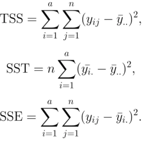
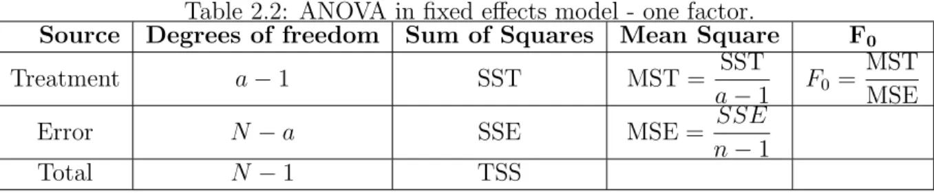
(30) Chapter 2. Background and literature review. 13. Where N = an it is the total number of observations. The hypothesis are H0 : µ1 = µ2 = · · · = µa versus H1 : µi 6= µj at least one pair (i, j). Sum of Squares. The sum of squares are needed to develop the test, the total sum of squares (TSS) in equation (2.5) is the sum of the squared di↵erences between the subgroup averages of the observed treatments and the grand average. The sum of squares due to the treatments is shown in equation (2.6). Equation (2.7) shows the sum of squares due to the experimental error. There are N = an observations. Thus, TSS has N 1 degrees of freedom. There are a treatments, SST has a 1 degrees of freedom. Finally, the SSE has n 1 degrees of freedom, where n represents the number of replicates. TSS =. a X n X. (yij. ȳ.. )2 ,. (2.5). i=1 j=1. SST = n. a X. (y¯i.. ȳ.. )2 ,. (2.6). i=1. SSE =. a X n X. (yij. ȳi. )2 .. (2.7). i=1 j=1. Mean Squares. Table 2.2 is called the analysis of variance table, in general, these are the steps to develop an ANOVA, the sum of squares are computed with the corresponding equations in this case the equations are (2.5), (2.6), (2.7), for the TSS, SST, and SSE respectively. The degrees of freedom are also computed for each of the sums of squares. To estimate the mean squares is needed to obtain the ratio of each sum of squares divided for its respective degrees of freedom. Once that the mean squares have been calculated, the ratio of the mean squares of the treatments divided by and the Mean squares of the error. Give the F0 value which will be used to compare it with the statistic to reject or not the null hypothesis. Also can be used to compute the p-value. The ratio is distributed as a F with (a 1) and (N a) degrees.

(31) Chapter 2. Background and literature review. Source Treatment Error Total. Table 2.2: ANOVA in fixed e↵ects model - one factor. Degrees of freedom Sum of Squares Mean Square SST a 1 SST MST = a 1 SSE N a SSE MSE = n 1 N 1 TSS. of freedom. Reject H0 if F > F↵,a 1,N hypothesis of the equality of treatments 2.1.4. 14. a. F0 MST F0 = MSE. otherwise do not reject the null. Model Adequacy. If the ANOVA model is considered for an application where we want to determine if there are or not di↵erences between the means of the treatments, we need to be sure that the model is appropriate for that application. For this, some assumptions need to be satisfied. These assumptions are that the model used, equation (2.1) or (2.2), describes the observations properly, and the errors follow a normal distribution with mean zero and 2 , where 2 is constant but unknown. If these assumptions are satisfied, the ANOVA is appropriate to test the hypothesis that the means of the treatments are equal. Though, in practice, it is common that these assumptions are violated. For this reason, it is convenient to verify the adequacy of the model for the data before inferences based on the model are undertaken. The aptness of the model can be proved with an analysis of the residuals. The residual of the j -th observation in the i -th treatment, and it is defined as eij = yij. ŷij ,. (2.8). where ŷij is an estimation of the observation ŷij and is obtained as ŷij = ȳ.. + (ȳi.. ȳ.. ).. (2.9). The analysis of residuals is required before conducting an ANOVA. If the residuals do not have a clear structure; it means that there is not a major concern, and it implies that the adequacy of the model is accomplished. A graphic analysis of the residual result is helpful to prove the aptness of the model..

(32) Chapter 2. Background and literature review. 15. Normality assumption. For the analysis of this assumption, normal probability plot residuals can be constructed. If the distribution of the residuals is normal, the plot will show a straight line, whereas a plot that departs substantially from linearity suggests that the distribution of the errors is not normal. Normality plots can also be used to detect outliers. An outlier is a residual that is bigger than any other. These outliers can introduce distortion in the analysis. Sometimes, the cause of an outlier is an measurement error; if this is the case, the observation can be deleted and the practitioner continue with the analysis without this observation. Independence assumption. Plot the residuals in the collection order helps to detect if there are any correlation between the residuals and time. If a positive trend is shown, it might suggest a positive correlation. This means that the independence assumption has been violated. The key to avoid this is to follow an adequate randomization process. Constant variance assumption. How was mentioned before, the residuals should not present a structure or a pattern, plot the residuals against the predictor variable is helpful to examine if the variance of the error terms is constant. Sometimes the constant variance of the observations is increasing when the observation increases. If this situation is present, the residuals the plot would show the data shaped like a megaphone. This could be occasioned because the data does not follow a normal distribution. This assumption is called homoscedasticity, that means, variance homogeneity (equality); if this assumption is violated, the type I error could be higher than the expected.There are statistics test that has been developed to test the equality of variances; these tests will be studied later. 2.1.5. Randomized Complete Block Design. When an experimenter is conducted, the variability induced by a perturbing factor may cause that the response variable is a↵ected. Sometimes, this factor is the one whose existent is not known and cannot be controlled. In other.

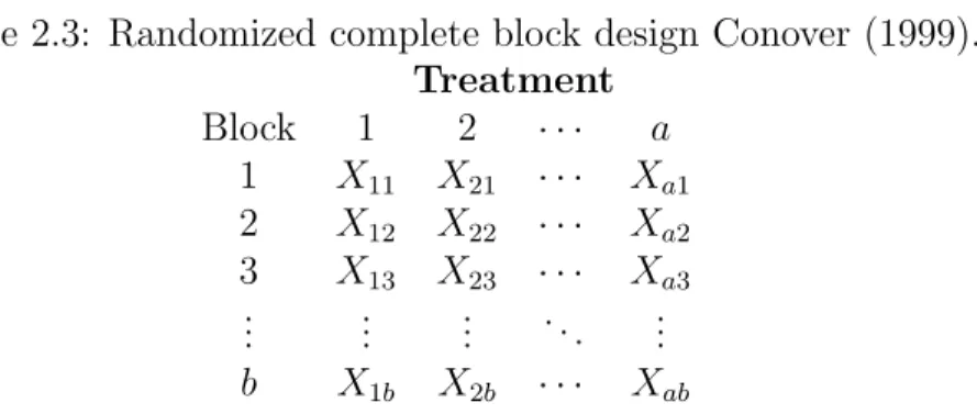
(33) Chapter 2. Background and literature review. 16. Table 2.3: Randomized complete block design Conover (1999). Treatment Block 1 2 ··· a 1 X11 X21 · · · Xa1 2 X12 X22 · · · Xa2 3 X13 X23 · · · Xa3 .. .. .. .. .. . . . . . b. X1b. X2b. ···. Xab. cases, its existence can be known, but is cannot be controlled. When this kind of factor is known and can be controlled, a technique called blocking can be used. This technique is used to eliminate the e↵ect caused by this nuisance factor when performing treatment comparisons. The principal objective of blocking is to make the experimental error as small as possible; to do this each block need to contain all the treatments; this is called complete. This design is known as a randomized complete block design (RCBD). This is a widely used design in practice. Suppose that you have a treatments that are going to be compared and b blocks. The RCBD is shown in Table 2.3. There is an observation per treatment in each block; the run order is random within each block. Statistical Model. The statistical model for the RCBD is yij = µ + ⌧i +. j. + "ij. (. i = 1, 2, ...a j = 1, 2, ...b. (2.10). where µ is the overall mean, ⌧i is the e↵ect of the i th treatment, j is the e↵ect of the j th block and "ij is the error term N (0, 2 ). In this model the e↵ects of the treatments and blocks are considered as fixed. These e↵ects are considered deviations from the overall mean, for this reason: a X i=1. ⌧i = 0,. b X j=1. j. =0. (2.11).

(34) Chapter 2. Background and literature review. 17. In practice, it is usually desired to evaluate whether treatment means are equal or not, and the corresponding null and alternative hypotheses are H 0 : µ1 = µ2 = · · · = µa H1 : Not all µi are equal. another equivalent hypothesis is to test in terms of the e↵ect of the treatment, the hypotheses are H 0 : ⌧1 = ⌧ 2 = · · · = ⌧a = 0 H1 : ⌧i 6= 0 at least for one i. The usual notation used when making calculations is yi. = y.j = y.. =. b X j=1 a X. yij. i = 1, 2, ..., a. (2.12). yij. j = 1, 2, ..., b. (2.13). i=1 a X X i=1 j=1. yij =. a X. yi. =. i=1. X. y.j. (2.14). j=1. where yi. are the observations in the i th treatment, y.j are the observations in the j th block and N = an it is the total number of observations. In a similar way ȳi. , ȳ.j , are the averages of the observations in the treatment and block respectively and ȳ.. is the grand average. Expressed algebraically ȳi. =. yi. , b. ȳ.j =. y.j , b. ȳ.. =. y.. . N. (2.15). The sum of squares are needed to develop the test, the total sum of squares (TSS) in equation (2.16) is the sum of the squared di↵erences between the subgroup averages of the observed treatments and the grand average. The sum of squares due to the treatments is shown in equation (2.17).The equation (2.18) shows the sum of the squares due to the block. Equation (2.18) shows the sum of squares due to the experimental error. There are N = an.

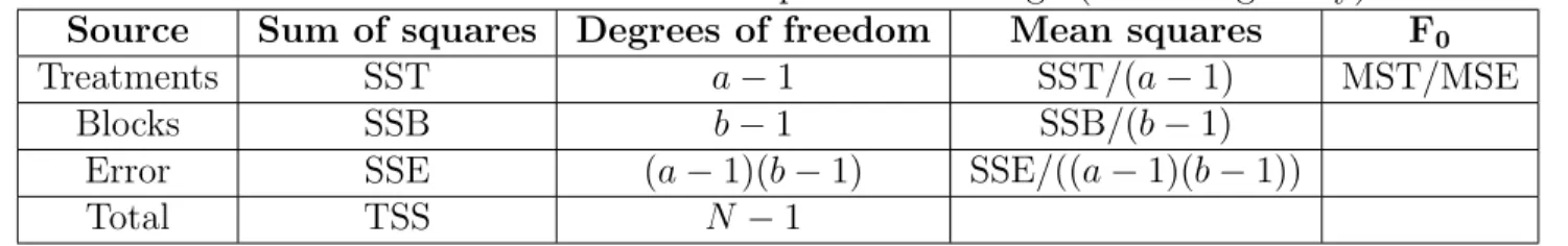
(35) Chapter 2. Background and literature review. 18. Table 2.4: ANOVA in a randomized complete block design (see Montgomery). Source Sum of squares Degrees of freedom Mean squares F0 Treatments SST a 1 SST/(a 1) MST/MSE SSB/(b 1) Blocks SSB b 1 SSE/((a 1)(b 1)) Error SSE (a 1)(b 1) Total TSS N 1. observations. Thus, TSS (2.16) has N 1 degrees of freedom. There are a treatments and b blocks, SST and SSB have a 1, and b 1 degrees of freedom respectively. Finally, the SSE has (a 1)(b 1) degrees of freedom. TSS =. a X b X. yij2. i=1 j=1 a. 1X 2 SST = y b i=1 i. b. 1X 2 SSB = y a j=1 .j SSE = T SS. SST. y..2 , N. (2.16). y..2 , N. (2.17). y..2 , N. (2.18). SSB.. (2.19). This corresponding ANOVA table is shown in Table 2.4. 2.2 2.2.1. Literature Review Previous works. Currently one of the key factors for the success of an industry is to use all the available tools, knowledge and experience that can contribute to the improvement of the company. The DOE is one of the tool for the optimization processes; this method can be defined as the realization of a set of tests for making changes to the variables under control of a process with the objective to observe and identify the reasons for the changes in the study and quantify it. The experiments are more complicated day by day because there are many factors that are subject to control and a↵ect the products and/or processes, hence there are many combinations of these factors that should be tested to obtain valid results..

(36) Chapter 2. Background and literature review. 19. Several tests have been proposed for the homogeneity of variances, the most frequently used are methods proposed by Bartlett (1937) and Box (1953). In this section, we describe these and other methods to test the homogeneity of variances that have been developed until now. The hypotheses to test we are interested in is H0 : 12 = 22 = · · · = a2 H1 : at least one i2 is di↵erent.. (2.20) (2.21). One of the most common tests to evaluate these hypotheses is the Bartlett test. This method includes a statistic whose distribution approximates a 2a 1 with a 1 degrees of freedom when the a are random samples from a normal population (Montgomery, 2008). The test statistic is 2 0. q = 2.3026 , c. where. a X. a)log10 Sp2. q = (N. (2.22). (ni. 1)log10 Si2 ,. i=1. c=1+. 1 3(a. 1). ✓X a. Sp2 =. (ni. 1). 1. (N. i=1. Pa. 1)Si2. i=1 (ni. N. a. a). 1. ◆. ,. .. Si2 is the sample variance. The null hypothesis is rejected when 20 < 2 ↵,↵ 1 . This test is sensitive to the normality assumption, for this reason is not recommended its use if normality is not sustained. Since the Bartlett test is sensitive to normality, other test have been developed. For instance, we have the modified Levene test known as the BrownForsythe test. This test is robust to deviations from normality. This test uses the absolute deviations of observations yij from the treatment median ỹi . This deviation is defined as ( i = 1, 2, ..., a, dij = |yij ỹi | (2.23) j = 1, 2, ..., ni ..

(37) Chapter 2. Background and literature review. 20. The modified Levene’ test is used to evaluate whether there are di↵erences in the mean of all the treatments. The test statistic is obtained by applying an F -ANOVA over the absolute di↵erences. Another test for variance was designed by Box (1953) to deal with nonnormal situation and k groups of independently distributed observations. The sample variance of each subgroup P 2 is computed. The estimated variance is 2 2 denoted by s , where s = is the total number of degrees of t st / and freedom. We then take the logarithm of the variance of each subgroup and obtain X 2 2 M1 = ln s t ln st . t. A k , where k is the number of subgroups, can be used to evaluate if the di↵erence in variance is significant. This statistic rely on large samples. For small samples, a correction is o↵ered by Box. When observations are not normal, the null distribution is adjusted using a function of the kurtosis. According to Bhandary and Dai (2013), the Box’s test has a weak power for the small sized data . A test for variance in a Randomized Complete Block Design was developed by Gill (1984) to give an exact criterion under the following conditions: • Error variance is di↵erent between treatments.. • Errors are correlated within a block but independent from block to block. With this assumption the test is executed, ignoring the heterogeneity of variances we found that the tabulated F is too low and hence we get significance. Thus we do not know if this is because there are really significance evidence or the large F is due to the heterogeneity of variances, for this reason, is difficult to draw conclusions about the treatments di↵erences. Conover et al. (1981) presented a comparative study of test for homogeneity of variances in their research. They provide a list of tests that have a stable Type I error rate when the normality assumption may not be true. Test with modifications of the likelihood ratio, modifications employing an estimate of kurtosis, modification of the F test and modifications of nonparametric tests are presented in this comparison study. Symmetric distribution like normal, and double exponential and asymmetric distributions such as uniform-squared, normal-squared and double-exponential-squared were used. Some of these test, such as Bar, Coch, and Hart, had an uncontrolled risk of.

(38) Chapter 2. Background and literature review. 21. Type I error when the populations are asymmetric. The principal findings are: • Three tests appear to have the best behavior in terms of robustness and power: Lev1:med, F-K:med 2 , and F-K: med F . • Replacing the treatment mean X̄ by the treatment median X̃ produced a significant decrease in the Type I error rate in some test. • The. 2. and F approximations resulted in almost identical test.. • Poor performance of most of these test when the distributions were asymmetric. • Test as Talwar-Gentle and FAB: med, never rejected the null hypothesis with a sample size (5,5,5,5). Bhandary and Dai (2008) developed a method that proves the equality of variance when the data are normal, following a multiple comparison procedure with correction for the global error. Some advantages are: (1) it is easy to perform, (2) there are no stringent requirements about the sample size, and (3) demonstrate good power in comparison with other tests such as Hartley, Levene and Bartlett’s tests. This test is sensitive to changes in the distribution. A test for the equality of variances in RCBD was developed by Bhandary and Dai (2013). This test is useful when there are larger number of treatments and small block size. Their test was compared with other eight test under the normality assumption. Test for homoscedasticity of variance have been developed using linear ranks such as (Conover et al., 2018) this research compared 66 variations of the test for equal variances and found that three of them were the most powerful. Tests were evaluated with Normal and Laplace, both symmetric distributions; and Normal squared, Laplace squared and Lognormal, skewed distributions..

(39) Chapter 2. Background and literature review. 22.

(40) Chapter 3. Methodology. 23. Chapter 3 Methodology 3.1. Mathematical Framework. To understand the problem under study, it is necessary to define a mathematical model and assumptions for the test we base our proposed test. The test used as a reference to develop this research is the Friedman test, which is an extension of the sign test, but using ranks to evaluate more than two treatments (Conover, 1999). This nonparametric test su↵ers of lack of power when only three treatments are compared, but its power increases when the number of treatments is more than four. This test is preferred to deal with the problem of comparing a di↵erent treatments, when a is greater or equal to 4. The design is an RCBD (see Subsection 2.1.5). This method is based on the ranks of the observations within each block. It is considered a two-way ANOVA with ranks with no interaction. There are b mutually independent blocks, a treatments, and each variables is defined as (X1j , X2j , ..., Xbj ), where j = 1, 2, ...a. The observation Xij is in block i and is associated with treatment j. It is necessary to obtain the ranks for each observation R(Xij ), the ranking is computed from 1 to b within each block (row) i, this means, each observation is compared with each other, and the rank 1 is assigned to the smallest value within block i, and so on until the a rank, that is for the largest observation. The ranking is computed for all the b blocks. In case of ties, use the average rank. After this sum of the ranks per treatment is calculate and we obtain Rj as follows.

(41) Chapter 3. Methodology. Rj =. 24. X. R(Xij ). j = 1, 2, ..., b.. (3.1). i. 3.1.1. Assumptions. A1. Observations between blocks are independent of each other. A2. The ranking is made within each block. 3.1.2. Friedman’s Test statistic. The statistic used in this test is: T2 =. (b 1)T1 b(a 1) T1. (3.2). where T1 is: (a. 1). T1 =. . Pa. 2 i=1 Ri. bC1. . A1 C 1 Rj is the sum of the ranks for treatment j and A1 and C1 are: b X a X. (3.3). [R(Xij ]2. (3.4). ba(a + 1)2 C1 = 4. (3.5). A1 =. j=1 i=1. 3.1.3. Friedman’s hypothesis and reject region H 0 : ⌧ 1 = ⌧2 = · · · = ⌧a = 0 H1 : ⌧i 6= 0 for at least one i.. (3.6) (3.7). T2 is approximately distributed as an F variable with (a 1) degrees of freedom in the numerator, and (b 1)(a 1) in the denominator (Conover, 1999)..

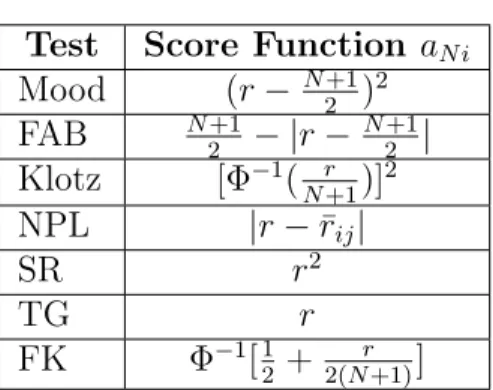
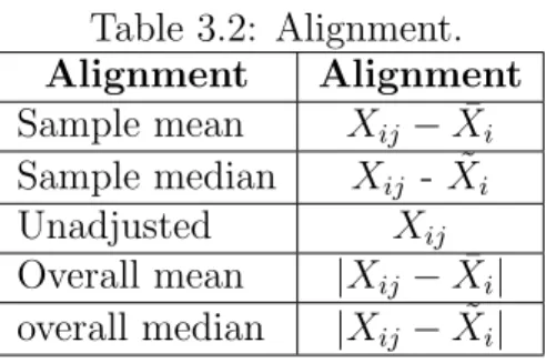
(42) Chapter 3. Methodology. 25 Table 3.1: Scores. Test Mood FAB Klotz NPL SR TG FK. 3.2. Score Function aN i (r N 2+1 )2 N +1 |r N 2+1 | 2 [ 1 ( N r+1 )]2 |r r̄ij | r2 r 1 1 [ 2 + 2(Nr+1) ]. Methodology. Using the Friedman ranking procedure, several nonparametric methods to test the equality of variance in an RCBD were developed. As we describe in Section 1, nonparametric tests can be created with the use of a rank transformation. In this case, we will use several data alignments and linear rank transformations (scores), as in Conover et al. (1981), to replace the simple rank transformation used by Friedman within each data block. Proposed steps to evaluate homoscedasticity are presented in the following subsections. A summary of the methodology is show at Subsection 3.2.4. 3.2.1. Select scoring type and alignment. Linear rank test from Conover et al. (1981) were adapted. First, a data a alignment is carried, and then a linear rank transformation, or scoring aN i , is used, where N is the sum of the individual sample size ni . This is shown in the tables 3.1 and 3.2 respectively. Table 3.3 shows a summary of the scorealignment combinations that were evaluated in this study. The 2 and the F statistics applied over the scores are described later. Next, a brief description of the test developed. The first test for the equality variance when the normality assumption is not accomplished, and the distribution is not known (nonparametric cases) was present by Mood (1954). In the nonparametric test, the null hypothesis assumes identical distributions and therefore equal means. Therefore Conover (1981) made an adaptation of this test and all the nonparametric test. Instead Mood.

(43) Chapter 3. Methodology. 26 Table 3.2: Alignment. Alignment Alignment Sample mean Xij X̄i Sample median Xij - X̃i Unadjusted Xij Overall mean |Xij X̄i | overall median |Xij X̃i |. Table 3.3: Tests statistics with the combination of scores and alignments. Test Mood sample mean Mood sample median Mood unadjusted FAB sample mean FAB sample median FAB unadjusted Klotz sample mean Klotz sample median Klotz unadjusted NPL sample mean NPL sample median NPL unadjusted SR sample mean SR sample median SR overall mean SR overall median TG sample mean TG sample median TG overall mean TG overall median FK sample mean FK sample median FK overall mean FK overall median. of letting Rij be the rank of Xij when the equality of means is presented or (Xij µi ) when there are not equal, let Rij be the rank of (Xij X̃i ). The Xij observation is replaced by a score of aN . This test results robust and powerful as some parametric test..

(44) Chapter 3. Methodology. 27. This test was introduced by Freund and Ansari (1957) and then modified by Ansari (1960), similarly to the Mood test, this is based on the scores (N + 1)/2 |Rij (N + 1)/2|; in this case apparently is a smallest variances, when the observations are closest to the median, and largest variances when are farthest from the median. FAB. A normal scores test by Klotz (1962) was introduced; this test uses the normal quantiles. It uses the Rij = (N + 1) quantile of the standard normal distribution. Klotz. A nonparametric version of Levene’s test was develop by Nordstokke and Zumbo (2010) this use the rank transformation by Conover (1981). The score is defined for the absolute of the di↵erence between the overall rank Rij , and the average of the ranks in that r sample is subtracted from each rank. NPL. The squared ranks test by Conover (2018), made the same deviation subtracting the Xij to the respective mean or median, and then obtain the squared ranks. SR. Talwar and Gentle Talwar and Gentle (1977) introduce this test, the result was a robust test to some nonnormal distributions. TG. Fligner and Killeen (1976) suggest the T-G test, in this use the normal scores from the positive half of the standard normal distribution. These are a list of test for variances, that appear to have controlled type I error, and these scores were used to develop this research. FK. 3.2.2. Test statistics. Four statistics were used to analyze the data of this research; two of them are obtained to approximate a 2 distribution and the other two for the F distribution. For the s statistics, the Friedman and Kruskal Wallis tests were used as a reference to obtain the 2F and 2K respectively. And these follow a 2 distribution with (a 1) degrees of freedom..

(45) Chapter 3. Methodology 2. 28. statistics 2 F. =. ✓. MST V ar(x). ◆✓. a. 1 a. ◆. ,. (3.8). 1)(SST) . (3.9) TSS Where MST is the mean squared of the treatment, var (x) is the sample variance, a is the length of the treatment, b is the length of the block, n is the number of replicates per cell, SST is the sum of squares of the treatment, and TSS is the total sum of squares In the case of the F statistics, the interaction or the absence of it was taken as a reference to obtain the Fone and Ftwo . First, in Fone the interaction between factors and blocks was not considered, so this statistic basically an adaptation of the F from a one-way ANOVA. Second, Ftwo considers the interaction from a two way ANOVA. They follow a F distribution: Fone with (a 1) degress of freedom in the numerator and (nba a) in the denominator; and Ftwo with (a 1), (n 1)(ba) degrees of freedom, respectively . The statistics are 2 K. =. b(na. F statistics. Ftwo =. TSS SST (nba 1) (a 1). SST. ,. (3.10). SST/(a 1) . (3.11) (TSS SST)/(nba a) where a is the length of the treatment, b is the length of the block, n is the number of replicates per cell, SST is the sum of squares of the treatment and TSS is the total sum of squares Fone =. 3.2.3. Hypothesis. Hypothesis This statistics test are used to prove the null hypothesis if the variances of the treatments are equal within each block. Hypotheses are:.

(46) Chapter 3. Methodology. 29. H0 : i = . . . = a = 0, H1 : At least one pair is di↵erent. 3.2.4. (3.12) (3.13). Summary of the proposed procedure. To test for homoscedasticity as defined in Subsection 3.2.3, the proposed methods follow: 1. Align your data as in Table 3.2. 2. Rank aligned data within blocks, as done by Friedman. 3. Apply a score function from Table 3.1. to the ranks. 4. Compute a test statistic as shown in Subsection 3.2.2. 5. Calculate the p-value using the corresponding null distribution associated with the test statistic in Section 3.2.2. 6. If the p-value  ↵, reject the null hypothesis. Finally, the R codes used to develop the simulations can be found in the following link: https://github.com/ptoram/NP-Test-for-homoscedasticity-withBlocks.

(47) Chapter 3. Methodology. 30.

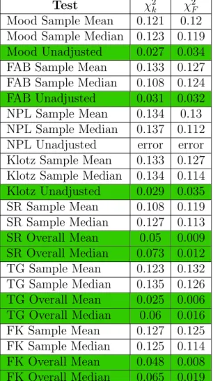
(48) Chapter 4. Results. 31. Chapter 4 Simulation Desing and Results. 4.1. Simulation Design. With the objective to obtain robust tests, a pre-selection of the tests were developed. Using a normal distribution and with the two test statistics for the 2 , 1000 simulations for each test were made in the software R. The first part of the analysis consisted in examining which test were robust. This is defined by Conover et al. (1981) as the probability of a type I error less than 0.10 for a 5 percent critical value. The test selected were the only ones with robustness, are shown in the Table 4.1. From the 96 di↵erent combinations of alignments, scoring and test statistics, we found robustness in only 9 alignment-scoring combinations with 4 test statistics, for a total of 36 tests. The same analysis was develop for the F statistics, and the results are the equal than for the 2 . The simulations were developed with 1000 simulations per scenario; the software used for this was R. Six di↵erent size or replicates per cell were used (2,5,10,20,50,100). A total of eight di↵erent combinations of main e↵ects ⌧ were evaluated, the first four for the sample size = 2, an the other four for.

(49) Chapter 4. Results. 32. Table 4.1: Initial assessment. Type I error probabilities over two are highlighted. 2 2 Test F k Mood Sample Mean 0.121 0.12 Mood Sample Median 0.123 0.119 Mood Unadjusted 0.027 0.034 FAB Sample Mean 0.133 0.127 FAB Sample Median 0.108 0.124 FAB Unadjusted 0.031 0.032 NPL Sample Mean 0.134 0.13 NPL Sample Median 0.137 0.112 NPL Unadjusted error error Klotz Sample Mean 0.133 0.127 Klotz Sample Median 0.134 0.114 Klotz Unadjusted 0.029 0.035 SR Sample Mean 0.108 0.119 SR Sample Median 0.127 0.113 SR Overall Mean 0.05 0.009 SR Overall Median 0.073 0.012 TG Sample Mean 0.123 0.132 TG Sample Median 0.135 0.126 TG Overall Mean 0.025 0.006 TG Overall Median 0.06 0.016 FK Sample Mean 0.127 0.125 FK Sample Median 0.125 0.114 FK Overall Mean 0.048 0.008 FK Overall Median 0.065 0.019. 2. statistics. Robust test. the sample size = 4: ⌧1 = (0, 0), ⌧2 = ( 1, 1), ⌧3 = ( 2, 2), ⌧4 = ( 3, 3), ⌧1 = (0, 0, 0, 0), ⌧2 = ( 1, 1, 1, 1), ⌧3 = ( 2, 2, 2, 2), ⌧4 = ( 3, 3, 3, 3). Three di↵erent size block amounts were considered: two, four, and eight.

(50) Chapter 4. Results. 33. blocks. For simplicity, all of these blocks were simulated with a main e↵ect of zero, as any given e↵ect is nullified by doing a within block ranking as the proposed methods under analysis. Eight di↵erent values were used, the first four for two treatments or samples, and the last four for four treatments or samples: = (1, 1), 2 = (1, 2), 3 = (1, 3), 4 = (1, 4), = (1, 1, 1, 1), = (1, 1, 2, 2), = (1, 1, 3, 3), = (1, 1, 4, 4). 1. 1 2 3 4. The distributions tested were the normal distribution with mean 0 and variance 1, the Normal squared distribution from a N (0, 1), double exponential distribution (also known as Laplace distribution), double exponential squared distribution from a Double exponential(0,1), Lognormal(0,1) distribution, a Gamma with a scale parameter of 1, and finally a Weibull with a scale of 1. For the distributions that require a shape parameter like Gamma and Weibull, four di↵erent values of the shape were used: 0.5, 1, 3, and 10. Table 4.1 shows all the score-alignment combination, and the highlighted rows are the robust tests. These were those who got a type I error probability less than 0.1. Only the 2 statistics were tested, these are the mentioned in subsection 3.2.2. All the combinations were tested with an alpha of 0.05. The procedure consisted in generating an scenario with each combination of distribution, replicate, treatment e↵ect, block, standard deviation, and test statistic, calculating the Rij ranks for each test. Then, a score function is obtained and the statistic tests based on the 2 and F statistic is computed. After obtaining all results, a selection of the best representation of the results was required, for this a amount of replicates per cell n = 5 was selected. This is because with this number of replicates, di↵erences between each test can be appreciate in a better way than if we increase it or decrease. From the simulation when n > 5, the powers were to high to easily detect di↵erences.

(51) Chapter 4. Results. 34. between tests. When n < 5, power was too low to detect di↵erences. When n = 5, di↵erences between tests were high enough to facilitate a conclusion. 4.1.1. Generate a scenario. Di↵erent scenarios were generated following the model Randomized Complete Block Design (RCBD) Xijk = µ + ⌧i +. j. + "ijk ,. i = 1, . . . , a; j = 1, . . . , b, k = 1, . . . , n.. (4.1). To generate the scenario with random observation, we can use the software R; the following arguments need to be specified: • n are the replicates per cell. • ⌧ are the e↵ect of the ith treatment is defined by the user. •. are the e↵ect of the j th block.. • Standard deviation, which is defined by the user. • µ is the mean. • Distribution, it can be choose for the following list. 1. Normal : Normal distribution. 2. Normal2 : Normal-squared distribution from a N(0,1). Basically a 2 with one degree of freedom. 3. DoubleExp: Double exponential distribution (also known as Laplace distribution). 4. DoubleExp2 : Double exponential squared distribution from a DoubleExp(0,1). 5. LogNormal : Lognormal distribution. 6. Gamma: Gamma distribution. 7. Weibull : Weibull distribution. • Others parameters that can be required are: – par.location: location parameter defined by the user usually is 0. – par.scale: scale parameter defined by the user usually is 1. – par.shape: shape parameter defined by the user usually is 0..

(52) Chapter 4. Results. 4.2. 35. Results. An analysis of symmetric distributions as Normal and Double exponential is presented. First, we o↵er the results for the symmetric distributions, and later for the skewed distributions Normal2, Double Exponential2, Lognormal, Gamma and Weibull. Although, for each distribution two tables are presented, one for the null hypothesis when there is no change in the standard deviation, and other for the average power when the standard deviation has changed. 4.2.1. Symmetric Distributions. Normal distribution null hypothesis. First, Table 4.2 shows the results for the normal distribution when the standard deviation does not have changes. In the case of two samples without changes in the mean, all tests are robust and the error Type I is under control for all blocks sizes. When there is a change in the mean, the test SR omedian increases but keeps its robustness. When there are four samples, and there is no change in the mean, all the tests are robust; but the tests FK omedian, SR omedian, and TG omedian showed sensitive to a change in the mean in all block sizes. Normal distribution power. Table 4.3 shows the results for the power with the Normal distribution when the standard deviation changed. When there are 2 samples all the tests have a good power, the most powerful statistics for di↵erent block sizes (2,4, and 8) were the Fone , in the case of 2 blocks the test that had the best behavior was the SR omedian, for 4 blocks was FK omedian and for 8 blocks were SR omean and SR omedian. When the number of samples increased to 4, the statistic F tends to be more conservative when the size of the blocks is small. The tests with more power were SR omedian, SR omean and FK omean for 2, 4, and 8 blocks, respectively. No changes in mean.

(53) Chapter 4. Results. 36. Table 4.2: Performance with the Normal distribution of di↵erent test homoscedasticity using statistics 2F , 2K , Fone , and Ftwo with 2,4, and 8 blocks when dealing with no changes in the mean of 2 and 4 treatments [(0 0) and (0 0 0 0), respectively], and changes in mean between 2 and 4 treatments [(-3 3) and (-3 -3 3 3), respectively]. All mean changes are measured in standard deviations of the null distribution. Treatment standard deviations are (1 1) and (1 1 1 1) for 2 and 4 treatments respectively. Mean. 00. -3 3. 0000. -3 -3 3 3. Test. 2 F. FAB unadj FK omean FK omedian Klotz unadj Mood unadj SR omean SR omedian TG omean TG omedian FAB unadj FK omean FK omedian Klotz unadj Mood unadj SR omean SR omedian TG omean TG omedian. .005 .004 .007 .002 .005 .006 .005 .003 .008 .000 .000 .000 .000 .000 .000 .000 .000 .000. FAB unadj FK omean FK omedian Klotz unadj Mood unadj SR omean SR omedian TG omean TG omedian FAB unadj FK omean FK omedian Klotz unadj Mood unadj SR omean SR omedian TG omean TG omedian. .000 .000 .000 .000 .000 .000 .000 .000 .000 .000 .000 .000 .000 .000 .000 .000 .000 .000. Normal distribution 2 Blocks 4 Blocks 2 2 2 F one Ftwo Fone F K K 11 .056 .048 .046 .006 .043 .071 .063 .049 .044 .010 .062 .067 .045 .046 .059 .010 .046 .048 .049 .062 .051 .004 .042 .056 .054 .046 .036 .005 .067 .076 .044 .066 .053 .004 .047 .054 .032 .056 .056 .003 .053 .061 .055 .067 .049 .008 .045 .070 .048 .055 .043 .007 .057 .072 .000 .000 .000 .000 .000 .000 .000 .000 .000 .000 .000 .000 .042 .064 .050 .002 .059 .060 .000 .000 .000 .000 .000 .000 .000 .000 .000 .000 .000 .000 .000 .000 .000 .000 .000 .000 .066 .070 .062 .004 .062 .097 .000 .000 .000 .000 .000 .000 .019 .034 .021 .003 .029 .048 1111 .049 .044 .051 .000 .061 .059 .043 .044 .047 .000 .042 .055 .053 .059 .044 .000 .049 .060 .031 .059 .042 .000 .055 .052 .041 .053 .038 .000 .056 .067 .046 .050 .051 .000 .066 .054 .029 .065 .038 .000 .046 .062 .043 .054 .051 .000 .046 .057 .044 .068 .056 .000 .048 .048 .016 .027 .020 .000 .026 .037 .022 .024 .023 .000 .021 .023 .097 .127 .132 .000 .126 .135 .013 .019 .012 .000 .015 .032 .019 .026 .014 .000 .022 .035 .022 .030 .017 .000 .031 .035 .135 .139 .142 .000 .121 .149 .022 .027 .019 .000 .028 .038 .103 .115 .113 .000 .119 .135. 8 Blocks 2 Fone K. Ftwo. .011 .003 .011 .011 .010 .011 .010 .006 .003 .000 .000 .013 .000 .000 .000 .012 .000 .001. .041 .046 .045 .045 .051 .046 .055 .048 .056 .000 .000 .044 .000 .000 .000 .075 .000 .051. .057 .075 .062 .064 .067 .060 .052 .056 .054 .000 .000 .076 .000 .000 .000 .064 .000 .034. .035 .030 .042 .044 .046 .051 .054 .063 .041 .000 .000 .055 .000 .000 .000 .076 .000 .029. .000 .000 .000 .000 .000 .000 .000 .000 .000 .000 .000 .000 .000 .000 .000 .000 .000 .000. .048 .037 .040 .044 .047 .048 .047 .046 .044 .024 .023 .108 .021 .031 .034 .125 .034 .122. .072 .064 .062 .061 .054 .061 .049 .047 .071 .028 .028 .143 .036 .034 .038 .139 .035 .121. .052 .058 .045 .058 .058 .052 .062 .056 .044 .024 .025 .139 .020 .016 .028 .153 .023 .132. Ftwo. 2 F. .056 .054 .055 .047 .056 .043 .041 .056 .045 .000 .000 .052 .000 .000 .000 .064 .000 .024 .045 .053 .040 .053 .054 .045 .053 .046 .060 .019 .027 .155 .010 .017 .027 .135 .022 .112.

(54) Chapter 4. Results. 37. For 2 samples, the tests that remain robust even if there are changes in mean are FK omedian, SR omedian and TG omedian over all statistics; and the most powerful test was the SR omedian over the three di↵erent block sizes. The statistics FAB unadj, FK omean, Klotz unadj, Mood unadj, SR omean, had good power when there was no change in mean, but, they lost power when there was a change in mean. When 4 samples were used, the best statistic was the Ftwo , and the test with better behavior was SR omedian. The test Mood unadj had good power when there was no change in the mean, but, was not sensitive when a change in mean occurred. Change in the mean. Double exponential distribution null hypothesis. The results obtained for the Double exponential distribution for the case, are shown in Table 4.4. For the sample size of two and without a change in the mean, all the tests have control of the error type I in all the cases of the number of blocks. But, the test FK omedian is sensitive to a change in the mean in the blocks size four and eight, and the SR omedian is sensitive in all the number of blocks. If the sample size increases to four and there is any change in the mean all the test are robust. The tests FK omedian, SR omedian, and TG omedian are sensitive to a change in the mean for all the sizes of the block. The statistics F has a conservative behavior when the sample increases. Double exponential distribution power. In Table 4.5 are shown the results for the power of the Double Exponential Distribution. When there are two samples all the tests have good power, the most powerful statistics for the di↵erent block size (2,4, and 8) is the Fone , the test that has the best behavior is FK omedian, for 2, 4, and 8 blocks. When the sample increases to 4, the statistic F tends to be more conservative when the size of the block are 2 and 4; the most potent tests are SR omedian for 2, 4, and FK omedian for 8 blocks. No changes in mean.

(55) Chapter 4. Results. 38. Table 4.3: Performance with the Normal distribution of di↵erent test homoscedasticity using statistics 2F , 2K , Fone , and Ftwo with 2,4, and 8 blocks when dealing with no changes in the mean of 2 and 4 treatments [(0 0) and (0 0 0 0), respectively], and changes in mean between 2 and 4 treatments [(-3 3) and (-3 -3 3 3), respectively]. All mean changes are measured in standard deviations of the null distribution. Treatment standard deviations are [(1 2), (1 3), and (1 4)] and [(1 1 2 2), (1 1 3 3), and (1 1 4 4)] for 2 and 4 treatments respectively. Mean. 00. -3 3. 0000. -3 -3 3 3. Test FAB unadj FK omean FK omedian Klotz unadj Mood unadj SR omean SR omedian TG omean TG omedian FAB unadj FK omean FK omedian Klotz unadj Mood unadj SR omean SR omedian TG omean TG omedian FAB unadj FK omean FK omedian Klotz unadj Mood unadj SR omean SR omedian TG omean TG omedian FAB unadj FK omean FK omedian Klotz unadj Mood unadj SR omean SR omedian TG omean TG omedian. Normal distribution 2 Blocks 4 Blocks 2 2 2 2 F F Fone Ftwo one two F K F K Average Power (1 2), (1 3), (1 4) .201 .446 .439 .475 .433 .690 .764 .694 .175 .498 .512 .491 .518 .781 .794 .786 .195 .537 .572 .556 .567 .785 .824 .796 .146 .462 .489 .478 .484 .745 .776 .733 .149 .484 .492 .480 .477 .744 .761 .745 .187 .517 .545 .504 .537 .771 .815 .779 .214 .560 .575 .562 .590 .800 .820 .806 .157 .450 .507 .452 .459 .728 .767 .721 .195 .507 .527 .533 .522 .743 .775 .759 .001 .020 .015 .021 .006 .022 .027 .022 .005 .027 .032 .030 .009 .060 .071 .054 .092 .478 .507 .466 .463 .744 .789 .756 .001 .011 .012 .010 .003 .012 .017 .018 .002 .010 .014 .011 .000 .015 .022 .018 .003 .035 .053 .039 .015 .082 .092 .078 .174 .544 .531 .528 .519 .771 .809 .776 .003 .019 .022 .022 .004 .033 .037 .028 .082 .367 .399 .366 .375 .678 .707 .659 Average Power (1 1 2 2), (1 1 3 3), (1 1 4 4) .000 .622 .673 .655 .091 .875 .896 .872 .000 .702 .739 .732 .107 .927 .934 .928 .000 .724 .747 .740 .135 .929 .935 .919 .000 .696 .729 .699 .040 .915 .933 .920 .000 .686 .722 .702 .117 .918 .916 .911 .000 .714 .734 .726 .149 .922 .935 .933 .000 .725 .756 .745 .186 .910 .933 .930 .000 .654 .701 .654 .102 .889 .903 .886 .000 .681 .695 .680 .138 .878 .899 .896 .000 .039 .054 .044 .000 .065 .074 .069 .000 .069 .075 .077 .000 .125 .147 .125 .000 .793 .815 .803 .210 .951 .951 .957 .000 .023 .038 .026 .000 .047 .049 .043 .000 .039 .042 .034 .000 .053 .056 .053 .000 .078 .103 .090 .000 .153 .181 .148 .000 .822 .828 .833 .303 .953 .957 .956 .000 .049 .053 .046 .000 .070 .073 .060 .000 .734 .752 .748 .181 .917 .927 .921. 8 Blocks 2 Fone K. Ftwo. .782 .842 .856 .818 .804 .855 .855 .798 .812 .013 .035 .808 .006 .005 .050 .827 .009 .717. .896 .937 .946 .920 .929 .944 .940 .925 .924 .042 .144 .926 .024 .041 .197 .938 .055 .886. .911 .951 .949 .941 .936 .953 .953 .927 .937 .058 .161 .941 .031 .048 .223 .947 .051 .900. .895 .929 .940 .925 .918 .946 .937 .919 .926 .041 .131 .919 .029 .031 .189 .933 .042 .887. .589 .665 .687 .656 .647 .681 .692 .600 .637 .000 .000 .792 .000 .000 .000 .835 .000 .719. .983 .995 .991 .995 .993 .996 .994 .986 .983 .134 .288 .996 .077 .101 .348 .996 .089 .993. .984 .997 .994 .995 .995 .994 .994 .991 .987 .146 .316 .997 .089 .115 .357 .998 .102 .992. .982 .997 .993 .992 .992 .997 .996 .984 .984 .131 .275 .997 .078 .091 .328 .999 .085 .991. 2 F.