Tuning of the dynamic model of a Linear Permanent Magnet Synchronous Motor in a positioning machine for metrology processes

Texto completo

(1)Instituto Tecnológico y de Estudios Superiores de Monterrey Campus Monterrey. School of Engineering and Sciences. Tuning of the dynamic model of a Linear Permanent Magnet Synchronous Motor in a positioning machine for metrology processes A thesis presented by. Julio Ruiz Carrizal Submitted to the School of Engineering and Sciences in partial fulfillment of the requirements for the degree of. Master of Science. In. Manufacturing Systems. Monterrey Nuevo León, Dec 10th, 2019.

(2) Dedication. To my Dear and Loving family, in special to my parents, Julio and Guadalupe, and my sister, Cristina.

(3) Acknowledgments. To my advisors for guiding me during this period and for their friendship To Tecnológico de Monterrey that supported me with tuition To CONACYT help me with my living expenses.

(4) Tuning of the dynamic model of an LPMSM in a positioning machine for metrology processes by Julio Ruiz Carrizal Abstract In this thesis, it is studied a dynamic force model for a Linear Permanent Magnet Synchronous Motor. A first approach to use the force model as a part of a Digital Twin is studied. The modeling was made from a machine designed to be a gauge machine for cold chamber die casting processes. It was determined the needed sensorization for running the model. The correspondent sensors were set in the machine during an experimentation session. Using several data processing algorithms as data filtering, interpolation, RMS calculation, and linear regression there were found normal operational parameters for a Linear Permanent Magnet Synchronous Motor present in the machine. From the analysis of different loads in the motor, a first approach for a performance monitor system was proposed..

(5) Index Chapter 1: Introduction ............................................................................................ 9 1.1. Background ................................................................................................ 9 1.1.1. Measurement System Project .............................................................. 9 1.1.2. Digital Twin Concept .......................................................................... 10 1.2. Problem Statement................................................................................... 11 1.3. Objectives ................................................................................................ 11 1.4. Scope ....................................................................................................... 12 1.5. Contribution .............................................................................................. 12 1.6. Document Organization............................................................................ 12 Chapter 2: Literature review .................................................................................. 14 2.1. Introduction .............................................................................................. 14 2.2. Digital Twin design ................................................................................... 14 2.3. Dynamic Force model .............................................................................. 16 2.4. Conclusion ............................................................................................... 18 Chapter 3: Methodology ........................................................................................ 20 3.1. Introduction .............................................................................................. 20 3.2. Experiments structure .............................................................................. 20 3.3. Operation motion test ............................................................................... 22 3.4. BackEMF Test .......................................................................................... 28 3.5. Data processing ....................................................................................... 29 3.6. Conclusion ............................................................................................... 30 Chapter 4: Results and discussion ........................................................................ 31 4.1. Introduction .............................................................................................. 31.

(6) 4.2. BackEMF Test .......................................................................................... 31 4.3. Operation motion test ............................................................................... 33 4.4. Discussion ................................................................................................ 39 4.5. Remarks ................................................................................................... 39 Chapter 5: Conclusion ........................................................................................... 41 5.1. Future Work ............................................................................................. 42 References ............................................................................................................ 44 Curriculum Vitae .................................................................................................... 44.

(7) LIST OF FIGURES. Figure 1. Measurement System CAD model ......................................................... 10 Figure 2.Current Sensor ........................................................................................ 24 Figure 3. Linear Encoder ....................................................................................... 24 Figure 4. Data Acquisition Board ........................................................................... 25 Figure 5. Galil’s motor controller............................................................................ 25 Figure 6. Diagram of experimental setup .............................................................. 26 Figure 7. Current sensing implementation ............................................................. 26 Figure 8. Test motor with 175 gr load .................................................................... 27 Figure 9. Schematic representation of motor’s movement .................................... 27 Figure 10. Back EMF test at 0.5 m/s ..................................................................... 32 Figure 11. Back EMF test at 0.25 m/s ................................................................... 32 Figure 12. Current measurements with no load..................................................... 33 Figure 13. Position graph ...................................................................................... 33 Figure 14. Current measurements filtered ............................................................. 34 Figure 15. Clark Transformation of filtered currents .............................................. 35 Figure 16. Park transformation of 2 phase currents .............................................. 35 Figure 17. Mobile rms current of current measurements filtered ........................... 36 Figure 18. Velocity graph of the motion experiment .............................................. 37 Figure 19. Acceleration graph of the motion experiment ....................................... 37 Figure 20. Comparation between measurement and model output ....................... 38.

(8) LIST OF TABLES. Table 1. Motor Specifications ................................................................................ 21 Table 2. Back EMF constant computation and percentual change ........................ 32 Table 3. Computed parameters with different masses .......................................... 38 Table 4. General computed parameters ................................................................ 38.

(9) Chapter 1: Introduction. 1.1.. Background. 1.1.1. Measurement System Project A new concept of a gauging machine was designed and built for pieces manufactured from a cold chamber die casting process. The new concept introduces the use of a laser sensor and a positioning system. With these changes, a more flexible system than the one being used at that moment was achieved. In addition, this new machine also incorporates several sensors like accelerometers, temperature sensors, and pressure sensors which proportionate environmental information and in a certain level performance information when the measurement process happens.[1], [2].

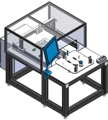
(10) Figure 1. Measurement System CAD model As part of the project, a system that connects the machine with a storage cloud system was developed and launched for when the machine was tested in a real plant. This system is constituted by a microcomputer Beagle Bone Industrial, the sensors installed on the machine, a wifi antenna, and the storage cloud system that it is a worksheet of google docs. The machine proved to be very repeatable with a value of 9.23 μm [2], which proved that the machine had the repeatability necessary to replace the current inflexible gauge system without affecting the quality of the measurement. While the data proportioned by the sensors in the machine and the possibility of cloud storage of that data were major contributions of the previous work, there is no procedure that allows determining the origin of the failures implemented. This limitation could result in low robustness during the normal operations of the machine.. 1.1.2. Digital Twin Concept According to the literature, a Digital Twin is a virtual representation of a system that can run different types of simulation which is characterized by the synchronization.

(11) between the real and the virtual system. A Digital Twin can be used to improve the system’s behavior doing the task of forecast and optimization. A digital Twin can be categorized by the level of integration of the digital model into the operation and communication with the physical model. The work presented three-level of integration: Digital Model, Digital Shadow, and Digital Twin. In the category of the digital. model,. there. is. only. a. mathematical/computational. model. that. represents/emulates the physical model. At this point of integration, there is no data flow between the digital model and the physical model in any direction. In the digital shadow category, a data flow from the physical model to the digital model exists. Finally, in the digital twin category, the data flow occurs in both ways.[3] 1.2.. Problem Statement. Currently, there are no methods or strategies implemented in the Measurement System to check the performance of the motors used in the machine movement. This makes it hard to determine the causes of the possible failures that can occur during operation- The literature presents dynamics models for a Permanent Magnet Linear Synchronous Motor (PMLSM), usually for controller design purposes.[4], [5] Also, there are examples of the implementation of digital twins for Permanent magnet synchronous motor (PMSM) in electrical vehicles[6]. But there is no implementation of a digital twin or shadow for a PMLSM. 1.3.. Objectives. The main objectives of this work are: •. Adapt a model for the force generated by the linear motors for monitoring proposes. •. Establish normal operating conditions. •. Develop a system to monitor motor/machine performance. The particular objectives of this work are: •. Determine which are required parameters for dynamic force model of a PMLSM. •. Design an experiment to determine the parameters of the model.

(12) •. Determine the numerical value of the parameters when the motor is operating normally and with the experimental results see how an unusual operation affects the parameters. •. Propose how the output of the model can be used as a monitor system for the performance of the motor. 1.4.. Scope. This work deals with the implementation of the current sensors required for the functionality of the digital model. The model can be used in controlled conditions to determine its parameters and compute the error in the modeling. The scope of this project is to get with a digital model for the motors in the machine, describe the sensors required to monitor its operations, and evaluate the digital model performance as a possible digital shadow. The way of the evaluation of the model is done through the comparison of the real measures and the computed outputs of the model. 1.5.. Contribution. In this work the main contribution is the use of a dynamic model for the forces in a PMLSM in join with current sensing and positioning sensing to get with a first approach to a digital shadow of the PMLSM in the machine, that can be useful in monitoring task and get closer to a digital twin implementation. 1.6.. Document Organization. This work is divided into five chapters. The content of each chapter is briefly described below: Chapter 2: Presents the solutions reported in the literature for problems that are close to the problem of design and put in operation a digital twin. Chapter 3: Describes all the experiments and data processing used to adapt the model to the measurements. Chapter 4: Presents the results of the experimental work and development of the models..

(13) Chapter 5: Presents conclusions about this work are done and it is presented the future work needed to produce a digital twin of the machine.

(14) Chapter 2: Literature review. 2.1.. Introduction. This chapter reports what can be found in the literature about Digital Twins. It is described the parts which are part of a Digital Twin. Furthermore, some applications of the digital Twins are described. Also, it is presented a case where a Digital Twin was applied as a monitor on a similar system that this work deals with. There are reported different dynamic models reported by diverse authors. Each author's approach and use of the model is described. 2.2.. Digital Twin design. The use of digital twins makes more responsive and predictive processes and helps with the developing of smart manufacturing.[7] The Digital Twins can make the process capable to react autonomously on new orders, modified order priorities or disturbances during operation.[8] The Digital Twin usually has targeted as increase competitiveness, productivity, and efficiency in fields like:.

(15) •. Production planning and control: Automatic planning and execution from orders by the production units. •. Maintenance: Identification the impact of state changes on upstream and downstream processes of a production system and/or identification and evaluation of anticipatory maintenance measures. •. Evaluation of machine: Process data during different stages of the machine life cycle to achieve better transparency of a machine's health condition. •. Layout planning: Continuous production system evaluation and planning. A digital twin can be described as a union between two systems. On one hand, there is a physical component, the physical model, which is the object to study. For that reason, several sensors are introduced to the physical model on it to obtain information about its progress, performance, or/and other important quantities relevant to the process itself that the physical model is doing. On the other hand, there is a digital model which is computer representation of the physical model normally using mathematic modeling to predict one or more important information of the physical value.[3] The union between the physical model and the digital model should happen to take the physical model measurements as agents of changes in the digital model which generates control instances to the physical model.[3] As mentioned before, one of the ways a digital twin can be used is as a system [3] that helps with the maintenance of a system. A digital twin was successfully implemented by Venkatesan et al [6] as a monitor system that allows to track the useful life in an electric motor for an electric vehicle using neural network and fuzzy logic for mapping inputs distance, time of travel of electrical. The digital twin is capable to simulate with this, operational parameters as casing temperature, winding temperature, time to refill the bearing lubricant, and percentage deterioration of magnetic flux..

(16) 2.3.. Dynamic Force model. The force developed for a PMSM can be obtained from the analysis of its electrical equivalent circuit.[9] Through the calculation of the currents from the voltage inputs in its terminals in a model like the one described by Equation 1 and Equation 2. 𝑢𝑑 = R𝑖𝑑 + 𝑢𝑞 = R𝑖𝑞 +. 𝑑ψ𝑑 𝑑𝑡 𝑑ψ𝑞 𝑑𝑡. − ωψ𝑞. (1). + ωψ𝑑. (2). Where ω: electric angular frequency ψ𝑑 , ψ𝑞 : direct and quadrature axis flux 𝑖𝑑 , 𝑖𝑞 : direct and quadrature axis current 𝑢𝑑 , 𝑢𝑞 : direct and quadrature axis voltage 𝑅: phase resistance Once solved for the currents and angular position the Toque can be calculated as a function of them. Appling the correct equivalences, the Toque can be calculated as a function of the quadrature current, the maximum magnetic flux of the magnet, and the angular position. To transform the analysis from a PMSM to a PMLSM it is usually used the π. equivalence θ = τ 𝑥, where τ, is half of the electrical cycle length. It can be appreciated as the distance between the magnets center lines. A model for a PMLSM is described in Equation 3 and Equation 4.[10] The dynamic force developed by the PMLSM is described by Equation 5. ud = Rid + Ld 𝑢𝑞 = R𝑖𝑞 + Lq 𝐹𝑚 =. 3π 2τ. did dt 𝑑i𝑞 𝑑𝑡. π. − τ vLq iq π. (3) π. + τ vLd id + ψ𝑓 τ v. 𝑝𝑝(ψ𝑓 𝑖𝑞 + (𝐿𝑑 − 𝐿𝑞 )𝑖𝑞 𝑖𝑑 ). (4) (5).

(17) Where 𝑣:. electric linear velocity. ψ𝑓 :. magnet flux. τ:. Pole pitch. 𝑖𝑑 , 𝑖𝑞 : direct and quadrature axis current 𝐿𝑑 , 𝐿𝑞 : direct and quadrature axis inductance 𝑢𝑑 , 𝑢𝑞 : direct and quadrature axis voltage 𝑅:. phase resistance. There is another way to modeling the force proportioned by PMSM in general. It is a non-simplified analysis. This model allows the modeling of an unbalanced motor, with practically any type of input signal. However, it requires the use of series to approximate all the harmonics that can affect the result. [11] For that reason, this model is not very used. The model described by Equation 1 and Equation 2 is used by Ohm D. [9] as the start of an analysis. Ohm explains the reason dq modeling is very used is that the model results be simple and intuitive besides the transformations. Ohm proposes methods to obtain the model parameters in several experiments. This work is explicit in how to obtain the parameters, but it does not provide an experimental example. For that reason, Ohm did not report accuracy in any of the model outputs. The model described by Equation 3, Equation 5, and Equation 6 Li T. et al [10] as a base to a control simulation. In this work, it is explained the importance of dq modeling in control applications. Basically, a PMLSM has one equation per phase, and each equation is strongly related to the main variables of the other phases. This makes impossible to control each phase separately. The dq model allows makes possible to apply the controlling doctrine to only quadrature current. The controlled quadrature voltage in combination with direct voltage can be transformed into its equivalent three-phase voltages. These voltages are the input of the motor. This.

(18) work presents a complete dq model for a PMLSM. It explains some of the typical controllers used with this model. However, the model is not explored as a monitor system to check performance. Alicemary et al [5] derived a similar model described by Equation 3, Equation 5, and Equation 6. Alicemary does several analogies with PMSM to explain the modeling of a PMLSM. The authors used the derived model to prove a nonlinear controller on a loop designed to control the dq currents. The authors derive practically the same model described by Equation 3, Equation 5, and Equation 6. They build a diagram block, block by block for everything, the dq voltage-current modeling and a motion model that takes care of mass and friction. The model is not explored as a monitor system to check performance. Faiz et al [4] use a similar model described by Equation 3, Equation 5, and Equation 6. The authors improve the control space vector modulation technique to reduce to minimize the total harmonic distortion. This improvement makes the system more efficient when there are load disturbances. The model is not explained as detailed as in the previous papers, but it is exactly the same. This means that the model is widely accepted as a good model for PMLSM. However, the model is not explored as a monitor system. Qin et al [12] use the model described by Equation 3, Equation 5, and Equation 6 in a complete gantry robot. The authors focus on the dynamic decoupling control method that they were developing. The developed control strategy allows the gantry system to reach the requirements of real-time and high precision performance for industrial applications. This work does not explore the model capacity to be a monitor of the performance of the motors in the robot. 2.4.. Conclusion. From the literature, it can be learned that the Digital Twins have important uses in the monitoring task and the maintenance task. In order to build a Digital Twin is necessary first to have a digital model of the physical system, later adapt the digital model to use as input real measures of the physical model. This achieves the second level of integration called Digital Shadow. As the final level of integration is necessary.

(19) to use the data generated by the digital model as part of the control inputs in the physical model. The literature also presents a wild use dynamic model called dq model. This model is principally used for simulation and control design. Few can be found about its use as Digital Shadow. There is an implementation of a Digital Twin in a similar system, PMSM. This Digital Twin is based on neuronal networks and fussy logic in its construction. Besides, it proves to have good results the final model misses the traditional modeling in the middle..

(20) Chapter 3: Methodology. 3.1.. Introduction. In this chapter, it is reported the followed methodology. All the experimental procedures are reported and the analysis of the obtained data. It is described the dynamic force model reported in the literature and an experiment which objective was to obtain a set of experimental data to compute the parameters of a dynamic motion model using a regression method. Later an experiment designed to obtain by another way a parameter of the force model, the back EMF of the motor, is described. later the calculated back EMF is compared with the one proportioned by the motor supplier. Also, it is documented all the devices used to run the experiment, and the data processing used in the data. 3.2.. Experiments structure. The force model that is tried to be characterized is one like the one described by Equation 5. Later it is made a simplification in the model. With this, the inductances.

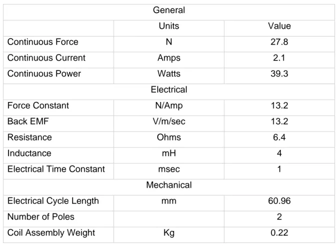
(21) are discarded from the needed parameters to run the force model. Also, it is described as the dynamic motion model used for the parameter’s calculation. This leads the task to determine all the needed parameters to run the models. For the Force model, the parameters can be obtained from Table 1. How the motor is not new, and it has been used in industrial environments, an experiment based on the measurement of the induced voltage was done to see the change on its parameters due to the use. Table 1. Motor Specifications General Units. Value. N. 27.8. Continuous Current. Amps. 2.1. Continuous Power. Watts. 39.3. Continuous Force. Electrical Force Constant. N/Amp. 13.2. Back EMF. V/m/sec. 13.2. Resistance. Ohms. 6.4. Inductance. mH. 4. msec. 1. Electrical Time Constant. Mechanical Electrical Cycle Length. mm. Number of Poles Coil Assembly Weight. 60.96 2. Kg. 0.22. The motion model parameters computation requires the measurement of the positions of the movement and the current measure. For that reason, the controller was configured to store position data. Also, a current sensing system was implemented..

(22) Using the experimental data, the correspondent transformations using Equation 8 and Equation 9 were tried as the method requires. At the same time, an alternative way to compute the current in the motor windings was performed. This data in join with the position encoder data is used to compute the movement model parameters. For the Back EMF constant test, the procedure followed starts with the calculation of the amplitude of the voltage signal. It follows a line-neutral to line-line voltage transformation using a conversion factor of √3. Once calculated line-line voltage it can use the formula to compute the Back EMF constant. Later, the calculated values are compared with the supplier’s value using the percentage change. 3.3.. Operation motion test. In the dynamic force model based on the dq analysis for an LPMSM, it is described by Equation 6. In this model, it is required to know the dq currents in the motor, the length of the electrical cycle of the motor, and the dq inductances of the motor. As a first approach, a balanced motor will be assumed. This means that 𝐿𝑑 = 𝐿𝑞 . With this assumption, the force model can be simplified as Equation 7. 3π. FE = 2 τ pp(λPM iq + (Ld − Lq )𝑖𝑑 𝑖𝑞 ) 3π. FE = 2 τ ppλPM iq. (6) (7). Where: 𝜆𝑃𝑀 :. Magnet flux. τ:. Pole pitch. 𝑖𝑑 , 𝑖𝑞 : Current at direct and quadrature axis 𝐿𝑑 , 𝐿𝑞 : Inductance in direct and quadrature axis This means that if it is desired to compute the dynamic force of the motor in the operation it is only necessary to determine the 𝑖𝑞 current via the complete motor modeling from input voltages measures, the currents. It also can be obtained measuring directly the current entering to the phases of the motor, which will be transformed to the equivalent 𝑖𝑑 and 𝑖𝑞 currents with the Clarke (8) and Park (9).

(23) transformation matrixes. These transformation matrixes work multiplying by the left the phase electrical currents as it is shown in Equation 10. 1. −. 1 2. 2 𝐾𝐶 = √3 0 1. √3 2 1. [√2. √2. 𝑐𝑜𝑠 𝜃 𝐾𝑃 = [ 𝑠𝑖𝑛 𝜃 0. −. 1 2. √3 2 1. −. √2. − 𝑠𝑖𝑛 𝜃 𝑐𝑜𝑠 𝜃 0. 𝑖𝑑 𝑖𝑎 [𝑖𝑞 ] = 𝐾𝑃 𝐾𝐶 [𝑖𝑏 ] 𝑖𝑐 𝑖0. (8). ] 0 0] (9) 1 (10). Where: π. θ= 𝑋 τ. 𝑋: Position from a magnetic zero 𝑖𝑎 , 𝑖𝑏 , 𝑖𝑐 : phase electrical currents 𝑖𝑑 , 𝑖𝑞 , 𝑖0 : electrical currents on direct, quadrature, and zero axis 𝐾𝐶 : Clark Transformation Matrix 𝐾𝑃 : Park Transformation Matrix 𝑖0 is known as the zero current because if the motor is balanced in its inductance and resistance phases, this current is always equal to zero. A set of three current sensors, one per phase, where installed on the cables that connect the motors with its controller. The sensor used in this experiment was the hall effect Tamura’s current sensors L01Z050S05. This sensor can measure currents until 50 A in both directions. It needs to be supplied with 5 Volts. The output of the sensor is connected in series with a 10 kΩ resistor. The reference voltage, where the current crossing the measurement zone is zero, is 2.5 V. When a current.

(24) cross its measurement zone a deviation from the reference voltage can be measured in the output with a sensibility of 33.3 A/V.. Figure 2.Current Sensor[13] To measure the motor position, the LM13 linear magnetic encoder system by RLS was used. It is a contactless high-speed linear magnetic with a 1 μm of resolution.. Figure 3. Linear Encoder[14] The recording data task is was done by an acquisition board NI USB-6210 by National Instruments for the current sensors. It was configured to obtain 10,000 samples at a rate of 1 kHz with a resolution of 153 μV..

(25) Figure 4. Data Acquisition Board The position recording task was done by the controller DMC-4143 by Galil Motion Control, Inc. The controller was configured to obtain data during the experiment at a rate of 500 Hz.. Figure 5. Galil’s motor controller[15].

(26) Figure 6. Diagram of the experimental setup. Figure 7. Current sensing implementation The controller was programmed to make three cycles of movement. The movement consisted of travel at a target speed of 0.5 m/s at a maximum acceleration of 2 m/s2 in a 55 cm travel. The experiment was repeated three times for six different loads. The purpose of having six different masses is to determine how a variation in the mass attached to the motor changes the model parameters. The test loads were 175 gr, 290 gr, 350 gr, 527 gr, 1.15 kg. To obtain these masses several iron plates were added to the motor like is shown in Figure 8..

(27) Figure 8. Test motor with 175 gr load The experiment deals with the movement of the motor along its axis. A schematic representation of motor movement is shown in Figure 9.. Figure 9. Schematic representation of motor’s movement FFigure 9 is derived from the model represented by Equation 11. 𝑑𝑉. 𝑀 𝑑𝑡 + 𝐵𝑉 + 𝐹𝑓 = 𝐹𝑚 Where: M: Moving mass 𝑉: Velocity B: Viscous friction coefficient Fm : Motor Force 𝐹𝑓 : Friction force. (11).

(28) 3.4.. BackEMF Test. The Back EMF is the voltage that appears in the motor terminals when it is moving. This effect is caused by the change of magnetic flux that crosses the windings of the motor. Equation 12 is known as faraday’s law. It describes the Back EMF of a winding as a function of the number of turns in the winding and the first derivate of the magnetic flux. 𝑉𝐵𝐴𝐶𝐾 = −𝑁. 𝑑Φ 𝑑𝑡. (12). Where: 𝑉𝐵𝐴𝐶𝐾 : Induced voltage 𝑑Φ 𝑑𝑡. 𝑁:. :. Rate of change of magnetic flux Number of turns in the winding. In practice, it is obtained the Back EMF constant using the measurement of the line to line voltage at a known speed. To calculate Back EMF constant, it is used the Equation 13. 2 Vline. λEMF = √3. ppv. (13). Where: 𝜆𝐸𝑀𝐹 : Back EMF constant 𝑉𝑙𝑖𝑛𝑒 : Line to Line voltage 𝑝𝑝: Pair of poles 𝑣: Linear velocity The supplier proportioned a value for the Back EMF constant of 13.2. 𝑉 𝑚⁄ 𝑠. how can be. seen in Table 1. However, when the experiment was run the motor was already subjected to industrial environments, so an experimental validation could determine a grade of wear..

(29) The experiment consisted of moving at two constant known velocities the motor while the line to neutral voltage was measured by an oscilloscope. The oscilloscope used during the experiment was a Keysight infiniiVision MSO-X 2014A. It is a four channels oscilloscope configured to record 5 seconds of samples at a rate of 50 kSamples/second. To measure the line to neutral voltage an electric plate where three resistors of 8.2 MΩ were connected in a star configuration was built. This configuration once connected to the terminals of the motor in motion creates a virtual neutral that allows taking the desired measure of line-neutral voltage for the three phases. 3.5.. Data processing. In the Back EMF test, the oscilloscope return filtered data, so it was only required to make an average of the amplitude of the motor's phases, change the voltage from line-neutral to line-line to finally apply Equation 12. For the operation motion test, it was necessarily making some operation to the data. The first operation was the synchronization of the data recollected from the DAQ and the controller. This was achieved by moving the starting point of the current data because the DAQ always started to record moments previous to the experiment. It was also required to filter the current data. This was performed by the Matlab function filter, which requires the coefficients of a filter in two arrays. The coefficients were calculated with the function “butter” of Matlab. The function returns the two arrays of coefficients for a discrete Butterworth filter. A 6-order filter was calculated for a cut frequency of 10 Hz. To determine the cut frequency a spectral analysis with an FFT was performed and it was seen that all the data was in the first 9 Hz. As a last processing method, it was used the mobile RMS calculation (14) to calculate the RMS current in periods of 100 ms. 1. 𝑥𝑅𝑀𝑆 [𝑖] = √𝑁 ∑𝑖𝑘=𝑖−𝑁+1 𝑥 2 [𝑘] Where:. (14).

(30) N: Window size x: Data i: Index 𝑘: Sum index 3.6.. Conclusion. The models used were described. Also, it is reported the methodology followed to determine the parameters via experimentation. It is documented the used sensors, the data processing used in the measurements, and the setup used in each experiment..

(31) Chapter 4: Results and discussion 4.1.. Introduction. On this chapter, it is presented all the experimental results. The Back EFM test results are presented on a graph of the phase voltages as measured in the test. For each speed tested, an average voltage amplitude was calculated to posteriorly be used on Equation 2. Then, a comparison is made between the value calculated from the experimental data and the one proportioned by the motor supplier. In the motion test, it is shown in several graphs' examples of how the data was collected, filtered, and the shifting that it was necessary to apply to current data. The computed values for three different variations of the model described by Equation 11 were reported in a table. Then, as the BackEMF Test, it is made a discussion of the results, how these parameters can be used as a monitor system, and its limitations. 4.2.. BackEMF Test. The phase voltage reported by the oscilloscope can be observed in Figure 10 and Figure 11. It can be seen how the test includes a round trip at two controlled speeds..

(32) Figure 10. Back EMF test at 0.5 m/s. Figure 11. Back EMF test at 0.25 m/s. Table 2. Back EMF constant computation and percentual change Speed. Avmean*√3. (m/s). Backemf. % of. (V/m/s). change. 0.25. 3.6655. 11.9714. 9.31. 0.5. 7.0524. 11.5165. 12.75.

(33) 4.3.. Operation motion test. The currents and positions taken from one of the experiments can be seen in Figure 12 and Figure 13.. Figure 12. Current measurements with no load. Figure 13. Position graph.

(34) The current data presented some noise in the measurement. For that reason, it was filtered with a 6 order Butterworth filter with a cut frequency of 10 Hz. The data filtered from Figure 12 can be seen in Figure 14. Figure 14. Current measurements filtered Once the current filtered and with the position information it is possible to apply the Clarke and Park transformations. In the Park transformation, the angle is calculated π. as θ = τ 𝑋. Where X is a distance from a zero magnetic phase. The positions were configured to make X = 0 coincide with a magnetic zero. Therefore, the position is directly applied to the angle relationship to later be used in Equation 9. The Clarke transformation of the currents shown in Figure 15 and the posterior Park transformation is shown in Figure 16..

(35) Figure 15. Clark Transformation of filtered currents. Figure 16. Park transformation of 2 phase currents The Park transformation should deliver signals that can be considered as dc or nonoscillatory. For that reason, to continue with the model analysis it was used the mobile RMS calculation to obtain graphs like Figure 17..

(36) Figure 17. Mobile rms current of current measurements filtered The disadvantage of the RMS calculation is due to the square operation in the formula the sign is loose. Because of that, It was only used the first movement to calculate parameters. How it can be observed in Figure 13 the position data does not present irregularities. So, it is not required any filtering. From this data, it was calculated the velocity and the acceleration with using a different method like the shown in Equation 15 𝑉𝑡 =. 𝑋𝑡 −𝑋𝑡−1 ∆𝑡. (15). Where Vt : Velocity at time t Xt : Position at time t. The velocity and the acceleration graphs from the position in Figure 13 can be observed in Figure 18 and Figure 19 respectively..

(37) Figure 18. Velocity graph of the motion experiment. Figure 19. Acceleration graph of the motion experiment How the Clark transformation could not be done properly, it was introduced a constant into the model to transform current to force and eliminates 𝐹𝑓 as it is shown in Equation 16. This was made to obtain a model with minimal variations when the mass varies. 𝑑𝑉. 𝑀 𝑑𝑡 + 𝐵𝑉 = 𝑘𝑖 𝑖𝑟𝑚𝑠 (16).

(38) As a first try to solve for the parameters, the model was solved for each of the different masses. Table 3 shows the best fits for each mass. Table 3. Computed parameters with different masses Mass 0. 0.175. 0.29. 0.35. 0.527. 1.15. 1.2255. 1.8023. 2.1469. 2.9291. 4.6139. 6.9894. B(N/m/sec) 0.5065. 0.7037. 0.8752. 1.2410. 1.9863. 3.0142. Error(N). 0.9036. 1.1241. 1.2198. 1.4790. 2.5537. K(N/Amp). 0.5803. A mass of 0.3 kg was added to each mass. This mas represents the motor's coil weight with a metallic plate that it has fixed to its body. To obtain a unique value for each parameter, the regression was applied to all the data.. Table 4. General computed parameters k. 2.0992. B. 2.7020. This last model was graph together with the measurement data in Figure 20.. Figure 20. Comparison between measurement and model output.

(39) 4.4.. Discussion. The constant Back EMF proportionated by the supplier is 13.2. 𝑉 𝑚⁄ . 𝑠. In both. experiments, this value results to be less than reported by the supplier as it is shown in Table 2. This can consequence of the time the motor was used before the test. However, the constant varies depending on the motor speed, and it can be observed that in one of the travels in both test there is one phase lightly higher than the others. These could be a symptom of an unbalanced behavior of the motor. In the motion experiment, the model is sensitive to the moving mass as can be observed in Table 3 and Figure 20. Also, the model presents an increasing error while more mass is charged to the motor. This effect can be caused by a misalignment in the ubication of the probe masses. Also, the changing mass due to the cables of the motor is not taking into consideration during the formulation of the model. With this model, it can be done basic monitoring by constantly solving the parameters of the model with new data. How it is known that the sensor mass is about 290 gr if the parameters start to deviate it can be associated with a change of the moving mass. How in the normal operation of the machine it is not a changing mass it means that something is in the close environment where the motor is moving. In that case, it would be reasonable to check the correct functionality of the motor. This means to check if there are obstructions in its path or lubricate its linear guides. 4.5.. Remarks. It is reported how the data looks when it was acquired. Following the described methodology in chapter 4 the measurements were processed. Later, the measurements are used to compute the parameters as the methodology explains. In the case of the calculation of the Back EMF constant, besides the value calculated reach percentual changes from the supplier value up to 12%, it can be explained due to the wear present in the motor. Nevertheless, the parameters found for the motion model presents big variations, up to 1.12 N when the sensor is mounted in the motor. As a first approach for a monitor system is proposed using continuous.

(40) solving for the motion model parameters to find variations associated first to mass variations..

(41) Chapter 5: Conclusion It was studied the definition of Digital Twins. It was determinate that it is required a series of steps in the level of integration of a digital model. In the literature can be found a dynamic model for PMLSM. It was determinate which parameters are required to run it. In order to calculate the needed parameters, two experiments were designed. All the needed sensors and equipment where implemented during an experimental session. The experiment used to calculate the BackEMF constant presented up to 12% variation with respect to supplier data. This can be explained as some type of motor wear and some unbalanced behavior. The motion experiment does not predict very well, but it can be used in a continuous computation of parameters as a monitor system. This based on an unexpected change of mass. For this system, the 290 gr would be considered as the parameters of the normal condition because 290 gr is the sensor’s mass. Stabilized the normal condition a monitor system can be implemented based on the changes in the model parameters based on unexpected mass variations..

(42) The difficulty to compute the dq currents in the Park transformation basically hinders the correct dynamic force modulation. Also, the calculation of the friction was not calculated by an isolated experiment. The objective of adapt a model for the force generated by the linear motors for monitoring proposes was reached. Either with the dq force model or the RMS approximation, the model can be feed with real data. Establish normal conditions was reached at some level, but it can be saying it was fully reached. This because a set of normal parameters were calculated, but the error in the predictions and an unexpected variation in mass are a symptom of that the model could be enhanced. With the same logic, the objective of developing a system to monitor motor/machine performance was not fully achieved because with a better motion modeling and a good current transformation it is expected a more intuitive model and with a better possibility to be used in a more complex model 5.1.. Future Work. It is necessary for the deepest comprehension of the dq model. This could be solving the problems in the second transformation. The voltage measure inclusion not only can solve the transformation problem but it can be used in the complete dq model to make predictions in the currents. The error in the current predictions can be used to determine the other parameters as the inductances and resistances. The knowledge of these parameters permits the use of the complete force model. The force prediction error can decrease dramatically. The parameter calculation in the motion model was not satisfactory with the least square regression method. So, it would be more precise design experiments that allow calculating each parameter alone to get a good start parameter. The use of the regression method can be used only in the monitoring prosses instead. Also, a basic model was proposed with no consideration of the orientation of the motor, the orientation of the load mass, and the changing cable mass is depreciated. A complete model taking these, and maybe other considerations could achieve a better parameter fit..

(43) In the literature, it can be found dynamic motion models for gantry robots as presented in [5], [16]. These means calculate some properties of the gantry as the mass and inertia moment of each link. Also, it must require to adapt the motion model to the proposes of monitoring..

(44) References [1]. A. P. Castro Martin, “Design of the technological infrastructure for data acquisition of an in-line measuring Industry 4.0 compatible machine,” Instituto Tecnológico y de Estudios Superiores de Monterrey, 2018.. [2]. D. F. Guamán Lozada, “Mechatronic Design of a Fast-Non-Contact Measurement System for Inspection of Castings Parts in Production Line.” 2018.. [3]. W. Kritzinger, M. Karner, G. Traar, J. Henjes, and W. Sihn, “Digital Twin in manufacturing: A categorical literature review and classification,” IFACPapersOnLine, vol. 51, no. 11, pp. 1016–1022, 2018.. [4]. J. Faiz, M. Manoochehri, and G. Shahgholian, “A novel robust design for LPMSM with minimum motor current THD based on improved space vector modulation technique,” Jt. Int. Conf. - ACEMP 2015 Aegean Conf. Electr. Mach. Power Electron. OPTIM 2015 Optim. Electr. Electron. Equip. ELECTROMOTION 2015 Int. Symp. Adv. Electromechanical Moti, pp. 1–7, 2016.. [5]. K. Alicemary, B. Arundhati, and M. P. Maridi, “Modelling , Simulation and Nonlinear Control of Permanent Magnet Linear Synchronous Motor,” vol. 1, no. 6, pp. 555–562, 2012.. [6]. S. Venkatesan, K. Manickavasagam, N. Tengenkai, and N. Vijayalakshmi, “Health monitoring and prognosis of electric vehicle motor using intelligent-digital twin,” IET Electr. Power Appl., vol. 13, no. 9, pp. 1328–1335, 2019.. [7]. Q. Qi and F. Tao, “Digital Twin and Big Data Towards Smart Manufacturing and Industry 4.0: 360 Degree Comparison,” IEEE Access, vol. 6, pp. 3585–3593, 2018.. [8]. R. Rosen, G. Von Wichert, G. Lo, and K. D. Bettenhausen, “About the importance of autonomy and digital twins for the future of manufacturing,” IFAC-PapersOnLine, vol. 28, no. 3, pp. 567–572, 2015.. [9]. D. Y. Ohm, “Dynamic Model of PM Synchronous Motors,” Drivetech Inc., pp. 1–10, 2000.. [10]. T. Li, Q. Yang, and B. Peng, “Research on Permanent Magnet Linear Synchronous Motor Control System Simulation,” AASRI Procedia, vol. 3, pp. 262–269, 2012.. [11]. Z. J. Gieras, Jacek F., Tomczuk, Bronisław Zbigniew, Piech, “Theory of Linear Synchronous Motors,” in Linear Synchronous Motors: Transportation and Automation Systems, 2012, pp. 107–151.. [12]. C. Qin, C. Zhang, and H. Lu, “H-shaped multiple linear motor drive platform control system design based on an inverse system method,” Energies, vol. 10, no. 12, 2017..

(45) [13]. T. C. Module Components Div, “Hall Effect Current Sensors L06P *** S05 Series Advantage : Hall Effect Current Sensors L06P *** S05 Series Mechanical dimensions,” no. March. pp. 5–6, 2012.. [14]. RLS merila tehnika, “LM10 linear magnetic encoder system,” no. 11. p. 10, 2011.. [15]. I. Galil Motion Control, “DMC-41x3 USER MANUAL.” 2016.. [16]. F. J. Lin, P. H. Chou, C. S. Chen, and Y. S. Lin, “Three-degree-of-freedom dynamic model-based intelligent nonsingular terminal sliding mode control for a gantry position stage,” IEEE Trans. Fuzzy Syst., vol. 20, no. 5, pp. 971–985, 2012..

(46) Curriculum Vitae Julio Ruiz Carrizal Date of Birth: November 27th, 1995 SUMMARY Mechatronics Engineer with specialization in supervision and control. I have experience in automation, mathematical modeling, and programing open-source electronic components. I have an interest in mechatronic design, sensorization, and machine design. EDUCATION Master of Science in Manufacturing Systems January 2018 – December 2019 Instituto Tecnólogico de y de Estudios Superiores de Monterrey Research Visiting. June 2019 - August 2019. Manchester University, Manchester, U.K. Bachelor in Mechatronics Engineering. August 2013 – December 2017. Instituto Tecnólogico de y de Estudios Superiores de Monterrey EXPERIENCE •. Software support - Expertis Debugging on programs used as GUI in communication with embedded devices. •. Investigator assistant - ITESM Design and test of an AGV prototype. SKILLS •. Languages: Spanish (Native), English (TOELF 600). •. Software: QtCreator, Flux, SolidWorks, Unigraphics, Labview, LtSpice, Fusion 360, Mathlab, Scilab, Arduino, C, C++, C#. HONORS/AWARDS.

(47) •. Honorable Mention and supervision and advanced control diploma by ITESM 2017. •. Scholarship to obtain the Master degree of Science in Manufacturing Systems granted by ITESM.

(48)