Pulsation regimes near static borders of optically injected semiconductor lasers

Texto completo

(1)Instituto Tecnologico y de Estudios Superiores de Monterrey Campus Monterrey School of Engineering and Science. Pulsation regimes near static borders of optically injected semiconductor lasers A thesis presented by Sergio Luis Rodriguez Martinez Submitted to the School of Engineering and Science in partial fulfillment of the requirements for the degree of Master in Science in Electronic Engineering. May 2018.

(2)

(3)

(4) DEDICATION. I dedicate this work to all my family, my mother Bertha, my father Sergio, my sister Lilia and my grandmother Dora and all my family.. iv.

(5) ACKNOWLEDGMENTS. I would like to thank my advisors, Dr. Gabriel Campuzano and Dr. Ivan Aldaya, for their encouragement, interest, and patience. Personally, I would like to thank them for sharing their knowledge which has enriched my study in lasers. I also would like to thank Tec de Monterrey for the support given by helping with the tuition and giving me a scholarship, and to CONACYT for the economical support given to me.. v.

(6) Pulsation regimes near static borders of optically injected semiconductor lasers by Sergio Luis Rodriguez Martinez. Abstract. The semiconductor laser injected externally by another laser (master-slave configuration) is a theoretical and experimental tool suitable for the scientific exploration of non-linear effects. Using numerical tools we have found pulsation regimes aside from period 1 and period 2. Techniques such as finding the maximum and minima of a temporal series, ratio between maxima and minima and the total harmonic distortion can be very useful to find and characterize pulsation regimes. Pulsation regimes where found near the borders of the stable synchronization region of the laser. The characterized region has a range of frequency from 150MHz to 2.78GHz with a frequency detuning from 0.98GHz to 3GHz.. vi.

(7) CONTENTS. LIST OF TABLES . . . . . . . . . . . . . . . . . . . . . . . . . . . . . . .. ix. LIST OF FIGURES . . . . . . . . . . . . . . . . . . . . . . . . . . . . . . . xii 1. Introduction . . . . . . . . . . . . . . . . . . . . . . . . . . . . . . . .. 1. 1.1. Justification . . . . . . . . . . . . . . . . . . . . . . . . . . . . . . . .. 2. 1.1.1. Generation of optical pulses . . . . . . . . . . . . . . . . . . .. 2. 1.1.2. Optical of electrical pulses . . . . . . . . . . . . . . . . . . . .. 2. Proposed technique based on optical injection locking . . . . . . . . . .. 3. 1.2.1. Hypothesis . . . . . . . . . . . . . . . . . . . . . . . . . . . .. 5. 1.2.2. Research questions . . . . . . . . . . . . . . . . . . . . . . . .. 5. 1.2.3. Objectives . . . . . . . . . . . . . . . . . . . . . . . . . . . . .. 6. 1.2.4. Contribution . . . . . . . . . . . . . . . . . . . . . . . . . . .. 6. 1.3. Organization of the document . . . . . . . . . . . . . . . . . . . . . . .. 6. 2. Pulse generation by cavity-enhanced FWM . . . . . . . . . . . . . . .. 7. 3. Methods . . . . . . . . . . . . . . . . . . . . . . . . . . . . . . . . . .. 8. 3.1. Rate equations (Detuning frequency, Injection Ratio) . . . . . . . . . .. 8. 3.2. Numerical solution method: Matlab ode45 . . . . . . . . . . . . . . . .. 9. 3.3. Method for pulsed regime identification . . . . . . . . . . . . . . . . . 11. 3.4. Method for pulse quality assessment (THD) . . . . . . . . . . . . . . . 18. 1.2. vii.

(8) 4. Results . . . . . . . . . . . . . . . . . . . . . . . . . . . . . . . . . . . 21. 4.1. Results of pulse generation . . . . . . . . . . . . . . . . . . . . . . . . 21. 4.2. Characterization of the pulses . . . . . . . . . . . . . . . . . . . . . . . 23. 5. Conclusions and discussion . . . . . . . . . . . . . . . . . . . . . . . . 31. 6. References . . . . . . . . . . . . . . . . . . . . . . . . . . . . . . . . . 32. viii.

(9) LIST OF TABLES. 1. Laser’s Parameters . . . . . . . . . . . . . . . . . . . . . . . . . . . . 10. ix.

(10) LIST OF FIGURES. 1. Free Running Laser . . . . . . . . . . . . . . . . . . . . . . . . . . . .. 4. 2. Master lasers starts pulling slave laser, before locking . . . . . . . . . .. 4. 3. Slave laser in locked mode . . . . . . . . . . . . . . . . . . . . . . . .. 4. 4. Experimental Setup of the optically injected semiconductor laser [1] . .. 5. 5. Temporal series ρ = −39.42dB ∆ωin j = 0.5GHz . . . . . . . . . . . . 11. 6. Contour of Minimum and Maxima ρ from -40dB to 10dB and ∆ωin j from -15GHz to 5 GHz . . . . . . . . . . . . . . . . . . . . . . . . . . 12. 7. Contour of optical peaks found ρ from -40dB to 10dB and ∆ωin j from -15GHz to 5 GHz . . . . . . . . . . . . . . . . . . . . . . . . . . . . . 13. 8. Contour of effective bandwidth ρ from -40dB to 10dB and ∆ωin j from -15GHz to 5 GHz . . . . . . . . . . . . . . . . . . . . . . . . . . . . . 14. 9. Contour of ratio ρ from -40dB to 10dB and ∆ωin j from -15GHz to 5 GHz . . . . . . . . . . . . . . . . . . . . . . . . . . . . . . . . . . . . 15. 10. Temporal series of Period 1 ρ = −10dB ∆ωin j = -5GHz . . . . . . . . 15. 11. Temporal series of Period 2 ρ = −32.98 dB ∆ωin j = -4.36 GHz . . . . 16. 12. Contour of the standard deviation. x. . . . . . . . . . . . . . . . . . . . . 17.

(11) 13. Contour of the mode . . . . . . . . . . . . . . . . . . . . . . . . . . . 17. 14. Contour of THD ρ from -40dB to 10dB and ∆ωin j from -15GHz to 5 GHz . . . . . . . . . . . . . . . . . . . . . . . . . . . . . . . . . . . . 18. 15. Comparison of Contours ρ from -40dB to 10dB and ∆ωin j from -15GHz to 5 GHz. 16. . . . . . . . . . . . . . . . . . . . . . . . . . . . . . . . . . 19. Contour of THD ρ from -40dB to -35dB and ∆ωin j from 0.5GHz to 3 GHz . . . . . . . . . . . . . . . . . . . . . . . . . . . . . . . . . . . . 20. 17. Contour of THD ρ from -40dB to -35dB and ∆ωin j from 0.5GHz to 3 GHz, yellow points show that the THD is greater than 1. . . . . . . . . 20. 18. Pulses ρ = −37.84dB ∆ωin j = -1.24GHz . . . . . . . . . . . . . . . . 21. 19. Pulses ρ = −39.42dB ∆ωin j = 1GHz . . . . . . . . . . . . . . . . . . 22. 20. Pulses ρ = −18.58dB ∆ωin j = -10.12GHz. 21. Pulses ρ = −23.08dB ∆ωin j = -6.44GHz . . . . . . . . . . . . . . . . 23. 22. Period of the pulses found in ρ = −39.42 . . . . . . . . . . . . . . . . 24. 23. Pulses found in ρ = −39.42 ∆ωin j = 1.4GHz . . . . . . . . . . . . . . 25. 24. Maxima and minima of the pulses found in ρ = −39.42. 25. Optical spectrum peaks of the pulses found in ρ = −39.42 . . . . . . . 26. 26. Ratio between maxima and minima of the pulses found in ρ = −39.42. 27. Total harmonic distortion of the pulses found in ρ = −39.42 . . . . . . 28. 28. Region ρ = −39.42dB with current equal to 7.5 times the threshold current. . . . . . . . . . . . . . . . 22. . . . . . . . . 25. 27. . . . . . . . . . . . . . . . . . . . . . . . . . . . . . . . . . . 29 xi.

(12) 29. Region ρ = −39.42dB with current equal to 11 times the threshold current. 30. Region ρ = −39.42dB with current equal to 13 times the threshold current. 31. . . . . . . . . . . . . . . . . . . . . . . . . . . . . . . . . . . 29. . . . . . . . . . . . . . . . . . . . . . . . . . . . . . . . . . . 30. Region ρ = −39.42dB first peak of optical spectrum with different currents . . . . . . . . . . . . . . . . . . . . . . . . . . . . . . . . . . . . 30. xii.

(13) 1. Introduction. Nonlinear dynamical systems are scientifically important in many areas of knowledge, such as biology, medicine, chemistry, physics, electronics, etc., because they constitute the theoretical framework for modeling a large diversity of phenomena with high spatio-temporal complexity[2]. The analytical and numerical tools developed over the last decades have triggered countless research efforts around the world with an evolved vision: originally the aim of studying nonlinear systems was to evade nonlinear distortion, whereas nowadays, the objective Has been expanded to exploit the nonlinear effects to the direct benefit of applications difficult to realize using linear systems. The area of optoelectronics has been an experimental pioneer in the development of nonlinear dynamics since it extends nonlinear optics to include the interaction of the optical field with the charge carriers within the semiconductors. The non-linear in the laser is attributed to the linear dependence of the gain in carrier density. By including this gain in the rate equations for the density of photons and carriers, the non-linear term emerges.. 1.

(14) 1.1. Justification. The interest of the study is not only scientific, but a number of new applications is seen in the areas such as optical processing [3], cryptography [4], emulating biological systems [5], random number generation [6], and remote microwave generation [7], etc.. 1.1.1. Generation of optical pulses. There are various techniques for generating optical pulses with lasers, the duration of the pulse can vary and could be in nanoseconds, picoseconds or femtoseconds . Such pulses can be used for many applications, such as telecommunications or ultraprecise measurements. Such techniques can be wavelength to time mapping (WTM) [8], long period fiber grating filter [9], super structure fiber Bragg grating [10], arrayed waveguide gratings [11], spatial light modulators [12], gain switching [13], Q switching [14], mode-locking [15].. 1.1.2. Optical of electrical pulses. To make optical pulses with electrical pulses the most common method in telecommunications is with modulators, The advantage of making pulses with optical injection locking is that high frequency electronics is not needed, and the frequency of the pulses can be controlled by just 2.

(15) adjusting the current in the master laser.. 1.2. Proposed technique based on optical injection locking. Injection locking is the result that takes place when an oscillator interacts with a second oscillator working at a close frequency. This occurs when the frequencies are near enough and the coupling is strong, the second oscillator can capture the first oscillator, causing it to have essentially the same frequency as the second [16]. The optical injection locking consists of a stable beam with a low power and a single mode spectrum from a master laser is injected to a high power slave laser. However, it is needed to use an isolator between the laser to prevent light from the slave laser being coupled to the master laser [17].In figure 4 can be observed the experimental setup where master laser is followed by the isolator,which prevents that the lights is reflected from the optical attenuator, then the light is injected to the slave laser. As we can see in figure 1 - 3, is the concept of injection locking, we have the free running laser, and when the light is from the master laser is injected, the master laser starts pulling the slave laser until reaching the locked frequency.. 3.

(16) Figure 2: Master lasers starts pulling slave Figure 1: Free Running Laser laser, before locking. Figure 3: Slave laser in locked mode. 4.

(17) Figure 4: Experimental Setup of the optically injected semiconductor laser [1]. 1.2.1. Hypothesis. Using the total harmonic distortion, number of maxima of temporal series, numbers of peaks in optical spectrum, and other techniques it is possible to localize regions of pulsations and characterize the pulses.. 1.2.2. Research questions. What injection ratio and frequency detuning is needed to get a pulsation regime? Where are the regions of stable synchronization (stable locking), period 1, period 2 or chaos? How depends the frequency of the pulses on detuning frequency?. 5.

(18) 1.2.3. Objectives. Look regions with interesting dynamics. Discover pulsation regimes. Localize the stable locking region Characterize pulsation regimes.. 1.2.4. Contribution. Characterize the pulsation regime found on the frequency detunings from 0.5 Ghz to 3GHz. With the pulse frequency, optical spectrum peaks, total harmonic distortion and number of maxima and minima of the temporal series.. 1.3. Organization of the document. First the four wave mixing will be explained, because is one of the reasons the pulsations occur at low injection ratios. Then the methods used will be shown, the rate equations and the laser parameters used for the simulation and the numerical solution parameters. The techniques for identifying the pulsation regimes will be discussed. Then different pulsation regimes found will be shown. Subsequently the region of focus is characterized by the techniques previously shown. Finally conclusions are presented.. 6.

(19) 2. Pulse generation by cavity-enhanced FWM. Four-wave mixing (FWM) is a non linear process that occurs by the third order nonlinear susceptibility χ (3) . If 3 optical fields with 2 or 3 different wavelengths propagate in a fiber simultaneously, χ (3) produces a new field that has a frequency ω4 related to the other frequencies of the fields [18].. ω4 = ω1 ± ω2 ± ω3. (1). The are various combinations for equation 1, by changing the plus and minus signs, but most of them are not possible because of the requirement of the phase matching. The most common is the degenerative case where ω1 = ω2 and has the form of ω4 = ω1 + ω2 − ω3. (2). This can be seen as two photons with energies of h̄ω1 and h̄ω2 are destroyed and the energy appears in the form of new photons with energies of h̄ω3 and h̄ω4 .. The four wave mixing inside a cavity is enhanced, since is experiencing a large enhancement of the nonlinear interaction efficiency. However, suffers from strong bandwidth constraints. As the cavity length is increased, the four wave mixing also increases, but the bandwidth decreases. [19]. 7.

(20) 3. 3.1. Methods. Rate equations (Detuning frequency, Injection Ratio). There is a set of 3 differential equations for optically injected lasers that is usually used [3, 20, 21, 22]. For a free running laser its complex field is described by the following equation, however it does not consider spontaneous emission.. 1 Ė(t) = g[N(t) − Nth ][1 + jα]E(t) 2. (3). Now for the optically injected laser equation is similar for the free running laser equation, just we need to add the injection terms.. 1 Ė(t) = g[N(t) − Nth ][1 + jα]E(t) + κAin j − j∆ωin j E(t) 2. (4). The equation 4 does not consider spontaneous emission, since it can be neglected because it is above the threshold. Langevin noises are also ignored. This equation can be split suppossing that E(t) = A(t)e jφ. 1 Ȧ(t) = g[N(t) − Nth ]A(t) + κAin j cos φ (t) 2. φ̇ (t) =. Ain j α g[N(t) − Nth ] − κ sin φ (t) − ∆ωin j 2 A(t). 8. (5). (6).

(21) Ṅ(t) = J − γN N(t) − [γP + g[N(t) − Nth ]]A(t)2. (7). Where A(t) is slave laser’s magnitude, φ (t) is the phase difference between master and slave, N(t) is the slave laser’s carrier number, g is the linear gain coefficient, Nth is the threshold carrier number, α is the linewidth enhancement factor,κ is the coupling coefficient, Ain j is the master laser’s magnitude, ∆ωin j is the detuning frequency between the master and slave, γN is the carrier recombination rate, and γP is the photon decay rate.. 3.2. Numerical solution method: Matlab ode45. For solving the rate equations of OIL, it was used a numerical solution using the Matlab R2017b software. The function used to solve the differential equation system is ODE45, which uses Runge-Kutta method of fifth order [23]. For the Runge-Kutta method it is only needed the initial conditions of the system. So for the initial conditions [22] we used for φ (t) 0, for N(t) Nth , and for A(t) it was used the magnitude of the free running laser A f r [22], which is defined as. s Afr =. 2. J − γN Nth γP. (8). The time used for the Runge-Kutta was 80 ns, and the number of points used was 65536. The relative tolerance was 1 × 10−9 .. 9.

(22) The injection ratio is defined in the following equation. Rin j = (. Ain j 2 ) Afr. (9). However its needed that the injection ratio be in a logarithmically scale for graphing purposes, so. ρ = 10 × log10 (Rin j ). (10). Laser’s Parameters. Value. units. Laser’s wavelength λ. 1550. nm. Linear Coefficient gain g. 5666.67. 1/s. Carrier number threshhold Nth. 2.214×108. #. Linewidth enhancement factor α. 3. -. Current J. 10×Jth. electrons/s. Current threshold Jth. 6.2414×1016. electrons/s. Carrier recombination rate γN. 109. 1/s. Photon decay rate γP. 3.333×1011. 1/s. Mirror Reflectivity r. 0.548. -. Coupling coefficient κ. 1.824 ×1011. 1/s. Table 1: Laser’s Parameters. 10.

(23) 3.3. Method for pulsed regime identification. One method used for the pulsed regime identification was the number of minimum and maxima of the temporal series of the laser, which is the how A(t) behaves over the simulation time. For example for the condition in figure 5 the laser, which is in stable synchronization, the number of minimum and maxima is 1, since the difference between points is so small after its transitory.. Figure 5: Temporal series ρ = −39.42dB ∆ωin j = 0.5GHz. Our region of interest was ρ from -40 dB to 10dB and ∆ωin j from -15GHz to 5 GHz. So a sweep was made with 251 steps in both ρ and ∆ωin j. 11.

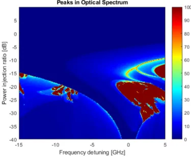
(24) Figure 6: Contour of Minimum and Maxima ρ from -40dB to 10dB and ∆ωin j from -15GHz to 5 GHz. Other technique used for the identification of the pulsed regime was the number of peaks of the optical spectrum of the temporal series, the temporal series where divided in two parts because at the start of the temporal series there is a transitory state, as we can appreciate at the start in figure 5, 10 and 11, so it is needed to remove that part and remain with the part of the temporal series that has only the repetition of the pulses (stable state). It is possible to observe in figure 7 that the darkest blue is the stable locking region, however the number of peaks increases to much in the zones around ρ = -20 dB and the frequency detuning of 3 GHz, this zone contains chaos, so the colorbar was capped to 100 peaks to be able to appreciate other zones. The number of peaks in the optical spectrum helps to identify regions of period one and period two. Since the. 12.

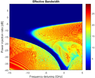
(25) optical spectrum is symmetrical it was only used half of it, so for period one instead of having two peaks in the spectrum, it has only one peak, the purpose of this was for increasing the speed of the simulation.. Figure 7: Contour of optical peaks found ρ from -40dB to 10dB and ∆ωin j from 15GHz to 5 GHz. Another technique was the effective bandwidth, which is defined [24]. f 2 Sd f −∞ Sd f. R∞. R∞ B = −∞. (11). Where B is the effective bandwidth, f is the frequency and S is the Spectral power density.. 13.

(26) Figure 8: Contour of effective bandwidth ρ from -40dB to 10dB and ∆ωin j from 15GHz to 5 GHz. The next technique used was the ratio between minima and maxima, to make this the temporal series was divided in a histogram of three segments, where the first segment was the minimum points, the third segment was the maximum points and the second segment was the rest of the points between the minimum and maximum. After half of the temporal series was classified in the histogram, the number of points of the third segment was divided over the number of points of the first segment. So if the ratio was to low or to high the region could be in a pulsed regime. In figure 9 it is possible to see period one in the light blue areas since the number of maxima is equal to the number of minima because it looks like a sine wave, see figure 10.. 14.

(27) Figure 9: Contour of ratio ρ from -40dB to 10dB and ∆ωin j from -15GHz to 5 GHz. Figure 10: Temporal series of Period 1 ρ = −10dB ∆ωin j = -5GHz. 15.

(28) Figure 11: Temporal series of Period 2 ρ = −32.98 dB ∆ωin j = -4.36 GHz. The last techniques used were the standard deviation of the difference of spacing between peaks in the optical peaks divided by the mean of the difference of spacing, and number of points of the spacing vector equal to the mode of the difference of spacing over the number of peaks. So for the standard deviation if it was close to 0, it can be a pulsed regime. For the mode if it was close to 1, it is close can be a pulsed regime. The contours are the following. 16.

(29) Figure 12: Contour of the standard deviation. Figure 13: Contour of the mode. 17.

(30) 3.4. Method for pulse quality assessment (THD). The total harmonic distortion (THD) is defined as the square root of sum of all the powers of the harmonic components over the power of the fundamental harmonic, defined in the following equation. [25, 26] p 2 T HD =. 2 ∑∞ n=2 In I1. (12). The THD will help to see the purity of periodicity of signal. If the THD is close to 0, then the signal will look like a sine signal. Since the desired signals are pulsed regimes, then the THD must be higher than 0. The same sweep was made for the THD so figure 14 was obtained.. Figure 14: Contour of THD ρ from -40dB to 10dB and ∆ωin j from -15GHz to 5 GHz. After this a comparison was made with figure 6 and 14. And a conditional was. 18.

(31) made for searching points that had THD greater than 1 and that had the minimum and maxima between 2 and 9.. Figure 15: Comparison of Contours ρ from -40dB to 10dB and ∆ωin j from -15GHz to 5 GHz. In figure 15 we can see the yellow colored points in the contour, which are the ones that had the accepted conditions. After this it was focus the bottom right yellow area which is around the 0.5 Ghz to 3 GHz, and making the same step jump, this will increase the resolution of the area, figure 16 was obtained. The points which had its THD greater than 1 where set to 20 to make contrast in the countour, as it can be seen in figure 17. 19.

(32) Figure 16: Contour of THD ρ from -40dB to -35dB and ∆ωin j from 0.5GHz to 3 GHz. Figure 17: Contour of THD ρ from -40dB to -35dB and ∆ωin j from 0.5GHz to 3 GHz, yellow points show that the THD is greater than 1.. 20.

(33) 4. 4.1. Results. Results of pulse generation. There were four areas that were highlighted, see figure 15, these areas present pulses of the following form, see figures 18-21. In figure 18 we observe downward pulses with an relaxation oscilation. In the other hand, in figure 19 we observe upwards pulses. In figure 20 and 21 are a combination of downward and upward pulses, but their amplitude is bigger compared to the other pulses.. Figure 18: Pulses ρ = −37.84dB ∆ωin j = -1.24GHz. 21.

(34) Figure 19: Pulses ρ = −39.42dB ∆ωin j = 1GHz. Figure 20: Pulses ρ = −18.58dB ∆ωin j = -10.12GHz. 22.

(35) Figure 21: Pulses ρ = −23.08dB ∆ωin j = -6.44GHz. We focus on the area to observe the region of ρ = −39.42 dB and the frequency detuning from 0.5GHz to 3 GHz. In this region the pulses are like the ones in figure 19. The pulses started appearing around the frequency detuning of 0.98 GHz, so before the 0.98 GHz is in stable synchronization.. 4.2. Characterization of the pulses. In figure 22 we can observe the period of the pulses found, the period starts very high in the frequency detuning near the border, and when the frequency detuning starts increasing, the period decrease rapidly but then slows down.. 23.

(36) Figure 22: Period of the pulses found in ρ = −39.42. In figure 24 it can be seen the number of maxima and minima of the temporal series, we can see that starts in 1, this is when the laser is in stable locking, but then starts increasing when it pases the border, however this starts oscillating between 4 and 6, this is because in the signal it can be seen the relaxation oscillation of the laser, as the frequency detuning increases, the relaxation oscillation starts to get disturbed by the signal, and the relaxation oscillation cannot be completed, this can be seen in figure 23. As the frequency detuning gets more far away from the stable synchronization region, the quality of the pulse starts decreasing. And transforms to a period 1 oscillation, this also can be seen in figure 24 since the number of maxima and minima gets to the value of 2 after the detuning frequency passes the 4.66 GHz.. 24.

(37) Figure 23: Pulses found in ρ = −39.42 ∆ωin j = 1.4GHz. Figure 24: Maxima and minima of the pulses found in ρ = −39.42. In figure 25, the optical spectrum peaks are shown, in the border the number of peaks increases drastically but then starts decreasing rapidly then slows down. The 25.

(38) number of peaks in the area of the detuning of 6 GHz and above remains as 4 or 3, even if the temporal series looks like a period 1 (sine wave) in the optical spectrum the fundamental peak appears with a very high intensity, but very small peaks appears in other frequencies. This is the effect of the master laser to pull the slave laser, but is not strong enough.. Figure 25: Optical spectrum peaks of the pulses found in ρ = −39.42. In figure 26 the ratio can be observed, the ratio between maxima and minima starts very low but starts increasing as the frequency detuning increases, however it does not remains around 1, it passes since the shape of the pulse changes, but the ratio remains low or high. However, after the frequency detuning of 4.66 GHz starts to decrease and tend to 1, because the temporal series start to be more like a period 1 oscillation (sine wave).. 26.

(39) Figure 26: Ratio between maxima and minima of the pulses found in ρ = −39.42. In figure 27, the total harmonic distortion is shown. The thd starts very high near the border of the stable synchronization, but decreases rapidly and remains oscillating around 1. So for this region the techniques used worked well and described the pulsation regime. For the frequency detuning of 4.66 GHz and above, the total harmonic distortion decreases and tends to 0 since the temporal series start to see more like a period 1 oscillation.. 27.

(40) Figure 27: Total harmonic distortion of the pulses found in ρ = −39.42. Finally the current J was changed, maintaing the same injection ratio and the same range of frequency detuning. The current J was equal to 10 times the threshold current in the previous case. Now we change the value of the current to 7.5, 11, 12,13,14,15, and 20 times to observe what happen to the frequency of the pulses, see figure 31. As the current was increasing, the stable locking region was moving to the right, however as the width of the stable locking region was becoming smaller and smaller. In figures 28-30, the spectrums of the region of ρ = -39.42 dB are shown. It can be observed in figure 31, that the frequency starts like an exponential but then it changes to an increasing straight line with a slope of 1, for the 7.5 Jth current the peak of the first spectrum in the detuning of 3GHz is almost in 3 GHz.. 28.

(41) Figure 28: Region ρ = −39.42dB with current equal to 7.5 times the threshold current. Figure 29: Region ρ = −39.42dB with current equal to 11 times the threshold current. 29.

(42) Figure 30: Region ρ = −39.42dB with current equal to 13 times the threshold current. Figure 31: Region ρ = −39.42dB first peak of optical spectrum with different currents. 30.

(43) 5. Conclusions and discussion. When ρ is on low values, the injected power of the light is not high enough, but still generates the FWM. If the detuning is close enough between the injected and the cavity .The pulsations occurs thanks to the four-wave mixing (FWM) and occurs inside the cavity, the FWM is enhanced and makes that frequential components appear since the master laser is pulling the slave laser. The techniques used, specially the number of minima and maxima, the ratio between the minima and maxima, and the total harmonic distortion, were really useful since they help us to find various pulsation regimes aside from period 1 or period 2, and can describe how a region behaves. In the analyzed region the frequency of the pulses found could vary from 150MHz to 2.78GHz by changing the frequency detuning from 0.98GHz to 3GHz. However as the frequency detuning increases and the more away is from the stable synchronization region, the pulses start to losing their quality, and starts transforming into a period 1 region, since the master laser is not able to pull the slave laser enough. The main application using OIL of this work could be a generator of optical pulses, and optical generator of pulses have various important applications like in telecommunications and other areas.. 31.

(44) 6. References. REFERENCES. [1] I. Aldaya, C. Gosset, C.Wang, G. Campuzano, F. Grillot, and G. Castanon, “Periodic and aperiodic pulse generation using optically injected dfb laser,” Electronic Letters, vol. 51, no. 3, pp. 280–282, 2015. [2] S. Strogratz, Nonlinear Dynamics and Chaos with Applications to Physics, Biology, Chemistry, and Engineering. Westview (Perseus Books Group), 1994. [3] S. Wieczorek, B. Krauskopf, T. Simpson, and D. Lenstra, “The dynamical complexity of optically injected semiconductor lasers,” Physics Reports, vol. 416, no. 12, pp. 1 – 128, 2005. [4] N. Li, W. Pan, L. Yan, B. Luo, M. Xu, Y. Tang, N. Jiang, S. Xiang, and Q. Zhang, “Chaotic optical cryptographic communication using a three-semiconductor-laser scheme,” J. Opt. Soc. Am. B, vol. 29, pp. 101 – 108. [5] F. T. Arecchi and R. Meucci, “Stochastic and coherence resonance in lasers: homoclinic chaos and polarization bistability,” The European Physical Journal B Condensed Matter and Complex Systems, vol. 69, no. 1, pp. 93–100. [6] P. Li, Y.-C. Wang, A.-B. Wang, and B.-J. Wang, “Fast and tunable all-optical physical random number generator based on direct quantization of chaotic self-. 32.

(45) pulsations in two-section semiconductor lasers,” Selected Topics in Quantum Electronics, vol. 19, no. 4, pp. 0600208–. [7] L. Goldberg, H. Taylor, J. Weller, and D. Bloom, “Microwave signal generation with injection-locked laser diodes,” Electronics Letters, vol. 19, no. 13, pp. 491– 493, 1983. [8] H. K. Chandrasekharan, F. Izdebski, I. Gris-Sánchez, N. Krstajic, R. Walker, H. L. Bridle, P. A. Dalgarno, W. N. MacPherson, R. K. Henderson, T. A. Birks, and R. R. Thomson, “Multiplexed single-mode wavelength-to-time mapping of multimode light,” Nature Communications, vol. 8, p. 14080, Jan 2017. Article. [9] D. Krčmařı́k, R. Slavı́k, Y. Park, and J. A. na, “Nonlinear pulse compression of picosecond parabolic-like pulses synthesized with a long period fiber grating filter,” Opt. Express, vol. 17, pp. 7074–7087, Apr 2009. [10] P. Petropoulos, M. Ibsen, A. D. Ellis, and D. J. Richardson, “Rectangular pulse generation based on pulse reshaping using a superstructured fiber bragg grating,” Journal of Lightwave Technology, vol. 19, no. 5, pp. 746–752, 2001. [11] T. Hirooka, M. Nakazawa, and K. Okamoto, “Bright and dark 40 ghz parabolic pulse generation using a picosecond optical pulse train and an arrayed waveguide grating,” Opt. Lett., vol. 33, pp. 1102–1104, May 2008.. 33.

(46) [12] A. M. Weiner, “Femtosecond pulse shaping using spatial light modulators,” Review of Scientific Instruments, vol. 71, no. 5, pp. 1929–1960, 2000. [13] K. Y. Lau, “Gain switching of semiconductor injection lasers,” Applied Physics Letters, vol. 52, pp. 257–259, Jan. 1988. [14] J. J. Degnan, “Optimization of passively q-switched lasers,” IEEE Journal of Quantum Electronics, vol. 31, pp. 1890–1901, Nov 1995. [15] R. Huber, M. Wojtkowski, and J. G. Fujimoto, “Fourier domain mode locking (fdml): A new laser operating regime and applications for optical coherence tomography,” Opt. Express, vol. 14, pp. 3225–3237, Apr 2006. [16] A. Pikovsky, M. Rosenblum, and J. Kurths, Synchronization: a universal concept in nonlinear sciences, vol. 12. Cambridge: Cambridge University Press, 2001. [17] I. Aldaya, J. Beas, G. Castanon, and G. Campuzano, “A survey of key-enabling components for remote millimetric wave generation in radio over fiber networks,” Elsevier, 2013. [18] G. P. Agrawal, Fiber-optic communication systems.. New York:. Wiley-. Interscience, 3rd ed., 2002. [19] F. Morichetti, A. Canciamilla, C. Ferrari, A. Samarelli, M. Sorel, and A. Melloni, “Travelling-wave resonant four-wave mixing breaks the limits of cavity-enhanced. 34.

(47) all-optical wavelength conversion,” Nature Communications, vol. 2, no. 1, p. 296, 2011. [20] R. LANG, “Injection locking properties of a semiconductor laser,” IEEE Journal of Quantum Electronics, vol. 18, no. 6, pp. 976–982, 1982. [21] C. Henry, N. Olsson, and N. Dutta, “Locking range and stability of injection locked 1.54 and 181 in ingaasp semiconductor lasers,” IEEE Journal of Quantum Electronics, vol. 21, pp. 1152–1156, August 1985. [22] M. C. Wu, C. Chang-Hasnain, E. K. Lau, and X. Zhao, “High-speed modulation of optical injection-locked semiconductor lasers,” Feb 2008. [23] Mathworks, “Ode45.” https://la.mathworks.com/help/matlab/ref/ode45.html accessed 2018-05-07. [24] H. E. Rowe, Signals and noise in communication systems. New Jersey: D. Van Nostrand, 1965. [25] I. V. Blagouchine and E. Moreau, “Analytic method for the computation of the total harmonic distortion by the cauchy method of residues,” IEEE Transactions on Communications, vol. 59, pp. 2478–2491, September 2011. [26] D. Shmilovitz, “On the definition of total harmonic distortion and its effect on measurement interpretation,” IEEE Transactions on Power Delivery, vol. 20, pp. 526–528, Jan 2005. 35.

(48)