Excitation emission matrices applied to the study of urban effluent discharges in the Chubut River (Patagonia, Argentina)
25
0
0
Texto completo
(2) One of the biggest problems that affected the water resources is pollution. In the case of South America about 50% of water used is extracted from aquifers, which are facing growing pollution caused by discharges of different types of industrial effluents [1]. The unrestricted use of rivers and estuaries to the discharge of different types of effluents result in significantly adverse effects. One is the phenomenon of eutrophication, this generic term defined as “the process of enriching water with nutrients (mainly nitrogen and phosphorus) that stimulate aquatic primary production” [2]. When the same is caused by man, it is known as cultural eutrophication and follows a series of events: Increased nitrogen and phosphorus, increased primary productivity, dissolved oxygen depletion, deterioration of water quality (increased turbidity and decreased light penetration) and development of algal blooms usually to the detriment of marine life [3,4] . The main cause of this phenomenon is the excessive release of nutrients into aquatic environments, especially in the form of untreated or inadequately treated discharges, which generally have high levels of organic substances. [2]. . These discharges can come from human. settlements, urban areas and certain industries, in addition to the contributions of agricultural and fish industries established in this area. In Chubut (Patagonia Argentina), the Chubut River is the most important water course, used not only for drinking water but also in agricultural irrigation and electric power generation (Dique Florentino Ameghino). All locations of the valley (Dolavon, Gaiman, Trelew, Rawson, Playa and Puerto Rawson Union) get their supply of freshwater in the Chubut River, as also do the discharges of agricultural wastewater, sewage and industrial effluents. It was considered important in the choice of effluent to be used, not just those from the sewage plant but also the processing fish plants in the Rawson city, which are discharged into the river near its estuary. This decision was based on two fundamental reasons: First, the volumes of water that the fish industries demand for its activity and second, the high content of dissolved organic matter that carry the effluent from this industry. Dissolved organic matter (DOM) is ubiquitous in aquatic systems and consists of complex mixtures of proteins and organic acids. They play influential roles in chemical.
(3) interaction within their environment and high levels of some organic substances can be considered pollutants. Traditional chemical analysis is not appropriate for efficient monitoring of the heterogenic nature of organic substances in natural and wastewaters. Dissolved Organic Matter (DOM) affects the functioning of aquatic ecosystems through its influence on acidity, trace metal transport, light absorbance and photochemistry, and energy and nutrient supply. [5]. . The principal source of DOM in surface waters is soil leaching. [6]. .. Furthermore, positive spatial relationships between Dissolved Organic Carbon (DOC) export and wetland areas like peat lands have been demonstrated [5]. Many potential factors (air temperature, increase in rainfalls intensity, atmospheric CO2 increase and decline in acid deposition) have been proposed to explain these trends in DOC, although there is no scientific consensus. Evans et al. (2005) have shown that recovery from acidification and water temperature are potential drivers, since many compounds forming part of DOC are acidic. In fact, a decrease in acid deposition is observed resulting partly from a decrease in anthropogenic sulphur emissions (industries, passengers/goods transportation) [7,8] . This could lead to an increase in soil pH and consequently to an organic acids increase permitted by new redox conditions. Nevertheless, trends in DOC are probably resulting from a combination of various factors, including acid deposition, since increasing trends have begun in a few places before reduction in acid deposition [9] . Fluorescence spectroscopy has become an important tool for additional characterization of organic matter over more general measurements such as dissolved organic carbon (DOC). Fluorescent spectroscopy has increased in the last decade with the development of synchronous fluorescence as a better tool for information on fluorophores in complex systems such as natural. [10,11]. and even more with excitation emission matrices (EEMs) that show the. joint variation the intensity and wavelengths of excitation and emission. In these complex systems, the emission spectrum may differ from the absorption. [12,13]. and the maximum. wavelength of emission is dependent on the excitation wavelength at which the spectra latter have limited utility. By contrast the EEMs can see the pair of wavelengths (or range of wavelengths) where the excitation and emission are highest (Exmax / Emmax) and this parameter or peak, is the distinctive feature of the fluorophores in question..
(4) There are a number of studies that have applied fluorescence spectroscopy to characterize industrial effluents and its flow toward various receiving bodies [10,14,15,16] . In aquatic environments, the DOM is composed of a variety of substances. Fluorescence spectroscopy has allowed characterizing DOM in samples of different origins. Two common uses of fluorescence spectroscopy in the analysis of aquatic environments are: 1) the study of organic compounds present in natural waters, such as humic acids, which are decomposition products of biological material generated by chemical and biological processes, and 2) the study of amino acids present in proteins and peptides (1, 2, 3). There are numerous papers in the literature which study dissolved organic matter (DOM) storage and redox state of fulvic acids in ground water beneath an island and riparian woodland (Mldanenov), the effects of many environmental stressors such as UV radiation are mediated by dissolved organic matter (DOM) properties (Mldanenov et al.), used to characterize dissolved organic matter (DOM) in water and soil (Chen, 2003), investigate the potential of detecting sewage pollution in a small, urbanized catchment using fluorescence spectrophotometry which allows the study of the DOM in the river (Baker, 2003) among others. Natural waters usually contain a mixture of fluorophors which make their identification difficult by means of unidimensional fluorescence spectra (Coble, 1996). An excellent analytical alternative is to measure fluorescence excitation-emission matrices (EEMs), which allow one to obtain richer information related to the presence and type of dissolved fluorophors. EEMs began to be studied in the decade of 1990, with the distinction of humic and non-humic compounds in natural waters (Coble, 1996, Coble et al., 1993, De Souza-Sierra, 1994). In order to extract information from the chemical components recorded in the EEM can be used different methodologies. One of the best known is the techniques such as parallel factor analysis (PARAFAC). Stedmon and Bro (2008) a description of the advantages and pitfalls of its application to DOM fluorescence is presented. PARAFAC enables decomposition of an EEM dataset into the least squares sum of several mathematically independent components, parameterized by concentrations (loadings) and excitation and emission spectra and corresponding, ideally, to a chemical analyte or group of strongly covarying analytes allowing the distinction between terrestrial and autochthonous organic matter sources in marine environments such (Murphy 2008). This algorithm allowed to identify humic and proteic substances in water samples (Kowalczuk et al., 2009), to characterize the DOM present in lakes.
(5) and soils (Fellman et al., 2009), to identify anthropogenic contaminants and metal traces in waters (Henderson et al., 2009), to study the discharge of effluents into rivers and marine waters associated with ranges of salinity and nutrients (Gao et al., 2010), to detect fulvic acids and tryptophan-rich proteins in sewage discharges (Mostofa et al., 2009), detect Fluorescence the presence of oxidized and reduced quinones in dissolved organic matter (Cory) and to classify water samples based only on the content of humic acids (Hall and Kenny, 2007). A related algorithm, multivariate curve resolution coupled to alternating least-squares (MCR-ALS) was also employed for similar purposes (Esteves da Silva etl al., 2006), study including fulvic acids in soils with different pH (da Silva, 2006), commercial humic acid, samples of fulvic acid (FA) extracted from a soil samples of FA extracted from recycled wastes (Antunes, 2005). Chubut River has been the subject of numerous studies as the primary source of freshwater in the province of Chubut. The Chubut River is embedded in a semiarid region of scarce water resources and has not been subjected to EEMs studies, except for a research. [17]. which applied. EEM fluorescence spectroscopy to the extracted humic compounds and not to the natural water samples. The former operation involves laborious isolation by processing large volumes of water. This work, however, focuses on the direct analysis of waters of the course, and on fish effluents and sewage discharges to the latter, in order to obtain information on the total composition of organic matter in the river water and the effect of the discharge. It is also the aim of this work to begin a survey with this new analytical tool as to the state of the Chubut River in an area near its estuary, comparing EMMS for natural freshwater and for freshwater impacted by discharge of effluents.. 2. MATERIALS AND METHODS 2.1. Description of the study area The Chubut river flows through the semiarid region of Patagonia Argentina and supplies drinking water to the towns of Dolavon, Gaiman, Trelew, Madryn and Rawson. The study of this course of water is therefore considered important from the environmental standpoint: it is used as a source of irrigation and drinking water across the lower valley of the Chubut River, and.
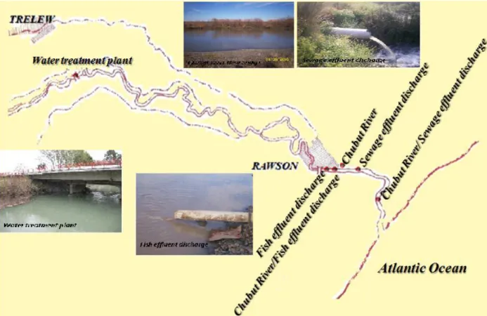
(6) is important from a touristic point of view, because it flows into the Atlantic Ocean forming the estuary at Puerto Rawson and Playa Unión, two areas for summer entertainment with coasts for recreation, fishing, water sports and sailing. The Chubut River Valley is located on the banks of the last 90 km of the Chubut River before emptying into the Atlantic Ocean. It has a surface of 40,000 ha, with a width varying between 7 and 10 km, of which 25,000 are watered. Approximately 900 producers operate in the area. The restricted study area is potentially influenced by fish and sewage discharges of effluents from Rawson city. A station upstream from the discharge (water treatment plant) (Fig. 1) was taken as a reference. Table 1 lists the sampling stations with their corresponding names, denominations and geographic locations obtained by GPS in the Chubut River area. 2.2. Sample Collection Water samples and effluent discharge samples were taken from subsurface, in some cases in areas prior to the discharge of effluents, and in other other cases post-discharge (Fig. 1). The sample of sewage discharge corresponds to the treatment plant in the Rawson city. A volume of 500 ml of water was taken for filtration and measurement of the fluorescence excitation-emission matrices. All samples were immediately transferred and processed.. 2.3. Laboratory Work 2.3.1. Filtration of samples Samples were filtered through filter GF/C (pore diameter 2 μm) and then through a Millipore nitrocellulose membrane with a pore diameter of 0.45 μm, previously washed with 100 ml portions of distilled water until no significant absorbance (range between 200 and 900 nm, as measured in a 10 cm quartz cell). 2.3.2. Physical and chemical parameters.
(7) For each sample, the in situ temperature (T) was measured and recorded, as well as the flow for each sampling station for the area. Conductivity 25°C (µS/cm)determinations were made using a Plessey conductmeter, pH determinations were carried out with a Hanna HI 8519N pHmeter, using an I1332 electrode, suspended solids (SS) were measured according to Standard Methods 2540D and sediment able solids according to the Standard Methods 2540F (APHA- AWWA-WEF, 1998) in unfiltered samples. Samples were then filtered through Millipore membranes (0.45 µm), previously washed until no significant UV absorbance was registered in a 10 cm quartz cell. The EEMs were recorded as detailed below, and the absorbance at 250 nm (A250) was measured with a Metrolab spectrophotometer. Absorbance measurements were performed with the purpose of knowing the degree of dilution which is needed to avoid inner filter effects in fluorescence measurements, and also as an organic matter indicator. [18,19,20]. . The samples from fish and sewage effluent had a dilution of. 20% and 10% respectively. Chemical Oxygen Demand (COD) determinations were made using DR2010 spectrophotometrically after closed digestion with potassium dichromate (Hach, Method 8000). Statistical analysis was performed by means of Excel 2003 and Sigma Plot version 8 programs. 2.3.3. EEM measurements EMMs were obtained, in a preliminary study, from concatenated emission spectra (between 280 and 700 nm) registered at different excitation wavelengths (220 to 520 nm) separated by 1 nm in both the excitation and emission dimensions. From these spectra, matrices were constructed by processing them with the Sigma Plot software version 8. Each matrix was corrected by subtracting a blank matrix recorded for distilled water, and obtained under the same conditions. A Shimadzu RFPC-530 spectrofluorometer with cells of 1 cm path length was employed for these preliminary measurements. Final EMMs were obtained using a Varian Eclipse spectroluminometer, using quartz cuvettes of 1 cm in the excitation range from 200 nm to 482 nm and emission range from 280 to 700 nm every 3 and 5 nm for excitation and emission respectively. The Raman intensity of pure water at the excitation wavelength of 350 nm was.
(8) controlled on a daily basis in order to obtain data at the same value of the source lamp. These matrices were then processed with Sigma Plot version 8.. 2.3.4. EEM deconvolution A discussion is presented on the use of a chemometric tool for the study of natural organic matter in conditions that characterize natural environmental systems. The algorithm multivariate curve resolution-alternating least-squares (MCR-ALS) was used to successfully decompose each single EEM into excitation and emission spectra for the detected components [21]. . If a given EEM (D) is of size JK, where J is the number of data points in the excitation. dimension and K the number of data points in the emission dimension, the bilinear decomposition of the matrix is performed according to the expression: D = Sexc SemT + E. (1). where the columns of Sexc contain the spectral excitation profiles of the intervening species, the columns of Sem their related emission spectra, and E is a matrix of residuals not fitted by the model. The iterative ALS procedure aims at minimizing the Frobenius norm of E, and is initialized using an initial estimation of the spectral or concentration profiles for each intervening species. Different methods are used for this purpose such as evolving factor analysis (EFA) the determination of the purest variables. [23,24]. [22]. or. . If the initial estimations are the spectral profiles. in the emission dimension, the unconstrained least-squares solution for the concentration profiles can be calculated from the expression: Sexc = D (SemT)+. (2). where (SemT)+ is the pseudoinverse of the spectral matrix SemT, which is equal to [Sem(SemTSem)−1] when SemT is full rank. [22]. . If the initial estimations were the concentration profiles, the. unconstrained least-squares solution for the spectra can be calculated from the expression: SemT = Sexc+ D where. Sexc+. (3). is the pseudoinverse of Sexc [Sexc+ = (SexcT Sexc)−1 SexcT], when Sexc is full rank. Both. steps can be implemented in an alternating least-squares cycle, so that in each iteration, new Sexc and Sem T matrices are obtained..
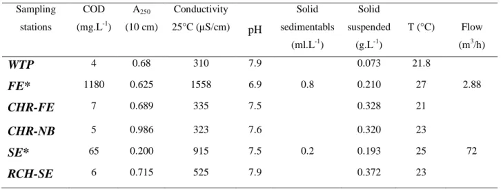
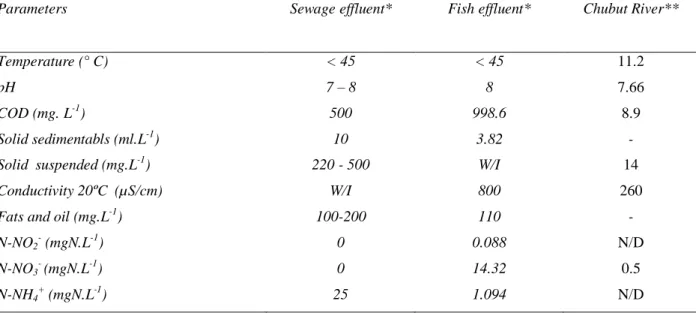
(9) During the iterative recalculations of Sexc and SemT, a series of constraints are applied to improve these solutions, to give them a physical meaning, and to limit their possible number for the same data fitting. [22]. . Iterations continue until an optimal solution is obtained that fulfils the. postulated constraints and the established convergence criteria. For example, non-negativity constraints are applied to the spectral profiles in both dimensions, due to the fact that the fluorescence spectra of the chemical species are always positive values or zero.. 3. RESULTS AND DISCUSSION 3.1. Environmental quality parameters of the water For assessing the physic-chemical quality of the reference area and the discharge of effluents, indicative parameters were measured for each sampling station (Table 2). Table 3 presents the comparison between the results obtained for fish and sewage effluents discharge in the influence area. This table summarizes the overall average parameters of fish and sewage effluent and existing data of Chubut River. Table 3 shows that the waters of the receiving body (Chubut River) are neutral or slightly alkaline, slightly mineralized, low in organic matter and suspended solids. Table 2 shows that the waters display constant conditions, with the exception of total and suspended solids, which increase both at the point of reference and downstream, indicating the previous existence of dragging phenomena of dissolved and particulate material. In relation to the sewage effluent from Rawson city, it can be observed that it shows a good degree of treatment at the plant in that city, because the COD value obtained in the analysis was well below expectations, a situation that is different for the fish effluent, which showed a high COD value. However, as regards the effect occurring in the overturning of both effluents of the Chubut River, the fish effluent has a very low flow and a minor impact on the receiving body. This can be concluded considering the low growth experienced by the river COD downstream of this discharge (Table 2). Table 3 shows that wastewaters from fish plants are characterized by large amounts of organic matter and suspended particulate, high levels of organic nitrogen and phosphorus, high BOD and generally have a characteristic grayish color. Organic pollutants consist of.
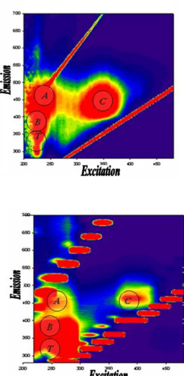
(10) carbohydrates, proteins, detergents and high fat content. Particularly associated with this is the fraction of tryptophan product of biodegradable materials.. Sewage effluent is composed of a heterogeneous mixture of compounds including fulvic acids, proteins, carbohydrates, lipids, organic surfactants, nucleic acids and volatile fatty acids varied [25].. 3.2. Fluorescence analysis During EEMs studies conducted in untreated sewage, a fraction of humic acids and protein fractions usually appear, corresponding to the amino acids tyrosine and tryptophan respectively [10]. The presence of these amino acids is common in waters with anthropogenic influence, such as bays, estuaries, coastal areas with high primary productivity, bacterial activity in water and effluent discharge areas are industrial and/or sewage, as in our working area. [26,27]. .. Fluorescence spectroscopy has enabled the distinction of the DOM from different sources [11,28,29]. , distinguishing, for example, the fluorescence of amino acids (primarily tryptophan,. tyrosine and phenylalanine) which are indicative of the presence of proteins and peptides with indol groups or other aromatic structures and has also been used to detect the presence of proteins in aquatic systems. Similarly, humic compounds allow the detection of fluorophores in the range of their emission maximum (420-450 nm). However, they differ in the excitation maxima, because one peak is stimulated at 230-260 nm and another one at 320-350 nm. The first peak is called A and the second one C. Also, depending on the studied environment, other peaks appear such as peak M, specifically related to marine salinity and the distance to the coast. Moreover, N, B, T and P peaks [30] are not humic type, but either protein type (B and T) or related to chlorophyll (P) or to the marine environment (N). The processed EEMs are presented for each sampling station with the corresponding fluorophores (Figure 2) according to the classification of Coble (1996) mentioned above. The EEMs for samples taken when the fish and sewage effluent are dumped into the receptor body are similar to those for the reference station, except that the protein bands are more intense (Fig. 2a y 2b). This comparison would indicate that the impacted water of the Chubut.
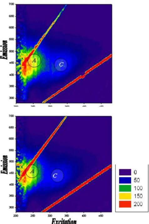
(11) River present a DOM composition having mainly humic compounds, and discharges of the type studied can be visualized by using fluorescence EEMs. Another noticeable issue is that the sewage effluent shows a greater concentration of the C fluorophore (Fig. 2c), which is the peak related to humic substances of allochthonous origin, a situation that seems to be logical, because of the contact with the water sludge treatment process. Unlike what is seen in the fish effluent, it presents a larger concentration of B and T fluorophores (Fig. 2d), corresponding to the protein fraction, and lower concentrations in the A peaks and C corresponding to humic substances. All samples, whether as such or as discharges of effluents mixtures with the Chubut river water, and samples from the Chubut River (Fig. 2e) and Trelew Water Treatment Plant (Fig. 2f), showed the A fluorophore (where the maximum excitation / emission is given in the range 237260/400-500) and a barely visible C fluorophore (where the maximum excitation / emission is given in the range 300-370/400-500). It must be stressed that these two fluorophores correspond to humic acids. Humic substances (HS) have properties with significant environmental effects(18) such as: 1) forming complexes with metal ions [31,32], influencing the cycle, transport and bioavailability of metals; 2) associating with organic pollutants. [33]. as pesticides and polynuclear aromatic. hydrocarbons; 3) affecting the growth of algae and bacteria disinfection products in the chlorination of drinking water. [34]. [35]. ; 4) generating carcinogenic. and 5) affecting the stability of. colloids [36]. From these properties the three last issues are important and should be highlighted in the area of study. While the Rawson water treatment plant is located upstream of the studied discharges, this zone corresponds to an area having a potential for recreational uses. Its use must be restricted to navigation, completely preventing the swimming in these waters. Regarding the relationship of HS and the growth of algae, there are studies that show the Chubut River inappropriate growth [37] of a particular algal species (Aulacoseira granulata) and species of dinoflagellates, both responsible for harmful algal blooms [38,39]. Studies in the lower section of the Chubut River, which show that this area has anthropogenic impact due to discharges urban, industrial and farming effluent (. Sastre et al.)..
(12) Among the species of toxic dinoflagellates can quote Alexandrium tamarense that is responsible for toxic events that force to impose bans on the collection of bivalves (Santinelli et. al, 2002). Also been found in this zone species produce toxins potentially diarrhea, as Dinophysis acuminata, discolorations or causing species such as Prorocentrum micans widely distributed in the Argentine Sea (Akselman et al., 1986). Massive growth (bloom) of cyanobacteria (bluegreen algae) in ponds, lakes, reservoirs or other freshwater systems have become serious water quality problems which also threaten human and animal health (WHO, 2003; Chorus and Bartram, 1999; Carmichael et al., 2001). Occurrences of cyanobacterial bloom typically appear in eutrophic lakes, which either have encountered anthropogenic nutrient loading or are naturally nutrient rich (Vaitomaa, 2006). Blooms of Microcystis species are known as one of the most common worldwide (Silva, 2003; Kann and Gilroy, 1997). The growth of Microcystis produces bad-smelling and unsightly scum, preventing recreational use of water bodies, hampering the treatment of water for drinking, and clogging irrigation pipe (Yoshinaga et al., 2006). As to the formation of carcinogenic disinfection products, it has been discussed in previous studies evaluating the potential formation of trihalomethanes, which was found to be below the limits accepted by the USEPA (100 mg / l), which coincided with those established by the Trelew Regulator. However, further studies are necessary because of the significance of this issue on the quality of the raw water (40). Natural organic matter (NOM) plays a significant biochemical and geochemical role in ecosystems and interest is growing concerning NOM occurring in water samples from both terrestrial and aquatic environments (Aiken et al., 1985; Dilling and Kaiser, 2002). One of the major problems related with NOM in the aquatic environment is the production of disinfection by-products (DBPs) such as trihalomethanes (THMs) and haloacetic acids (HAAs) during water treatment and supply. In studies, it was observed that the disinfection by-product formation potentials (DBPFPs) of the humic fraction (i.e., HS) in natural surface water were significantly high, compared to the DBPFPs of the non-humic fraction (Kim et al., 2004a,b). NOM including HS is one of the known predominant precursors of DBPs formed during chlorination in water treatment processes (Bellar et al., 1974; Rook, 1974), many studies have.
(13) been conducted into decreasing the DBPFPs through removal of NOM. However, since HS characteristics from specific natural water depend highly on the geochemical and environmental conditions of the watershed, it is important to investigate the characteristics of HS to establish an optimal treatment strategy for DBPs control. These points are considered important because of the occurrence of A and C fluorophores for humic substances mentioned above, according to observations based on the measurement of EEMs for samples taken in the Chubut River and Trelew Water Treatment Plant. It is also important to emphasize that the results found in this study agree with some authors who believe that tryptophan fundamentally occurs with high intensity in the EEMs, due to the fact that it is the result of anthropogenic material in raw water and untreated effluent or primary treatment. (10, 14, 15, 16). . Moreover, other authors associate the presence of this amino acid. with the growth of bacterial communities. (11, 41). . These amino acids are characteristic of fish. effluents origin, because of their prevalence in the material used. The fluorescence of proteins in aquatic environments is the result of a mixture of autochthonous and allochthonous sources. Thus, the presence of tryptophan and tyrosine is common in waters with anthropogenic influence such as bays, estuaries, coastal areas with high primary productivity, bacterial activity in water and effluent discharge areas (both industrial and/or sewage) (26, 27).. 3.3. MCR-ALS analysis The results obtained by the deconvolution of the matrices, implementing the MCR-ALS model, allow to differentiate humic substances and proteins present in natural complex samples. These initial studies were performed by Cobles (42) and De Souza-Sierra (12).Then, advancements in fluorescence spectroscopy allowed to determine different types of humic substances and proteins, depending on their emission/excitation ranges. In our case, the A and C fluorophores, which have the same emission maximum but different excitation maxima, are recognized by the MCR-ALS model as a single component. The same applies to B and T fluorophores, which only differ in their emission spectra. However, by inspection of the excitation (or emission) spectra of that single component, it was possible to observe the characteristics of each fluorophore (either A/C or B/T), which are present in the form.
(14) of a linear combination, with a greater proportion of the component that produces the greatest signal. Another issue that was considered is the percentage of variance which is explained by the MCR-ALS model. This parameter was satisfactory in most samples, except in those where the fluorescence signal was too low in comparison with the noise and with other spectral artifacts such as the Rayleigh (first- and second-order) and Raman dispersions. In the case of the Chubut River and Trelew Water Treatment Plant, where we observed the presence of the A and C fluorophores detected by measuring the EMM data, the deconvolution suggests the existence of the predominance of A over the C fluorophore. The MCR-ALS model yields 97.8% and 98 % of explained variance respectively by considering only one main component, which coincides with the mentioned fluorophores: component 1(type A) with 97.8 % and 98 % to the Chubut River and Trelew Water Treatment Plant respectively Taking into account that MCR-ALS cannot differentiate fluorophores that have the same emission and a different excitation spectra, the presence of A and C fluorophores cannot be distinguished. However, the deconvolution demonstrates the superiority of humic substances over bio-based materials. In relation to fish and sewage effluents, where the EEM shows a mixture of fluorophores (A, B, C and T), the MCR-ALS model explains a variance of 99.9% with 2 main components to the sewage effluent, with a 98.7 % for component 1 (A fluorophore) and 1.2% for component 2 (T fluorophore). Similarly, for the fish effluent sheds the explained variance was 84.2% with 2 components, consisting of 74.9% for component 1 (T fluorophore) and 9.3% for component 2 (A fluorophore). It is important to remark, in relation to what was found in the wastewater effluent, that the model does not allow the distinction between A and C fluorophores, both having a very high fluorescence intensity. Although the deconvolution results indicate the presence of a single major component, due to the intrinsic characteristic of the sample, this major component should correspond to C, which represents humic substances of allochthonous origin linked to contact with these sludge treatment plants in the waters of the liquid sewage. As regards fluorophore T, it is important to note that it is present as a main component for both types of effluents. In the case of the sample corresponding to the fish effluent, it is the first component, a situation that seems to be logical given that it represents tryptophan-rich protein.
(15) amino acid, the fundamental basis of the raw material used in the manufactur process of the fish industry. For the discharge of sewage and fish effluents on the receiving body (Chubut River), the MCR-ALS model yields an explained variance of 99.9% with 2 main components to the case of discharge of sewage: Component 1 with 99.8% (A fluorophore) accord to the humic substances that are the priority for the MOD fraction of the river, and component 2 with 0.12% (T fluorophore) characteristic of sewage. For the fish effluent, MCR-ALS provides 86.4% of explained variance, also with 2 main components: Component 1 with 86.1% (A fluorophore) and component 2 with 0.3% (T fluorophore). The results are consistent with the above discussion, bearing in mind the low flow of this effluent compared to the sewage effluent, which could indicate a lower impact of these effluents into the waters of the Chubut River. It can be concluded that fluorescence spectroscopy, particularly excitation/emission matrices (EEMs) have a high potential for its application to the study of OM in natural waters and anthropogenic impacts. They also allow to study and research sources, nature and reactions that occur in relation to aquatic organisms, as well as studying the behavior of the MOD in industrial effluents and sewage into aquatic waters. It also has a potential for the characterization and quantification of NOM present waters, either as allochthonous autochthonous sources, and to obtain relations between fluorescence and other techniques to monitor water quality from both chemical and biological standpoints. This correlation test can be rapidly performed to analyze water quality, to track pollution or contaminated areas and to detect anthropogenic activity in certain areas in relation to other areas in their natural state.. 4. CONCLUSIONS Excitation-emission matrix fluorescence spectroscopy can be considered as a good indicator of the environmental changes under the influence of external factors such as the discharge of industrial effluent, sewage or spill of any type of hydrocarbon. Furthermore, we consider it as a good parameter for the observation of the change, according to the nature of what gets into the environment. As well as, for characterization of industrial effluents or sewage.
(16) through a methodology that is sensible, simple and rapid. Finally, using these matrices through fluorescence enabled a rapid and specific analysis of the study area, giving the possibility to evaluate the type of problem and ensure monitoring of contaminated areas, allowing the distinction between the impacted areas and those that are taken as the reference area and occur in nature. 5. REFERENCES 1- I. Delpla, A.V. Jung, E. Baures, M. Clement and O. Thomas. Environment International 35: 1225–1233 (2009). 2- R.A. Vollenweider, A. Rinaldi and G. Montanari.. Science. of. total. Environments.. Suplement: Marine coastal eutrophication 63-106 (1992). 3- M.T. Gomoiu. Science of total Environments. Suplement: Marine coastal eutrophication (7) 151-152 (1992). 4- M. Aubert. Science of total Environments. Suplement: Marine coastal eutrophication 615-629 (1992). 5- C.D. Evans, D.T. Monteith. and D.M. Cooper. Environments Pollution 137: 55–71. (2005). 6- J. Hejzlar, M. Dubrovsky, J. Buchtele and M. Ružička M. Sci Total Environ 310: 143152 (2003). 7- D.T. Monteith, J.L. Stoddard, C.D. Evans, H.A. de Wit, M. Forsius and T. Høgåsen. Nature 450: 537–41 (2007). 8- C.D Evans, D.T. Monteith, B. Reynolds and J.M. Clark. Sci Total Environ 404: 316–25 (2008). 9- F. Worrall and T. Burt. J Hydrol. 346: 81–92 (2007). 10- A. Baker and R.G.M. Spencer. Science of the Total Environment 333,1.3 (2004). 11- W.K.L. Cammack, J. Kalf, Y.T. Prairie and E.M. Smith. Limnology and Oceanography 49, 6 (2004). 12- M.M. De Souza-Sierra, O.X.F Donard, M. Lamote, C. Bellin and M. Ewald. Mar. Chem. 47, 127 (1994). 13- P.G. Coble. Marine Chemistry 51, 4 (1996)..
(17) 14- R.P. Galapate, A. Baes, K. Ito, T. Mukai, E. Shoto and M. Okada. Water Research 32, 7 (1998). 15- D.M. Reynolds. Water Research 37, 13 (2003). 16- A. Baker, R. Inverarity, M. Charlton and S. Richmond. Environmental Pollution 124, 1 (2003). 17- M.C Scapini, A. Olivieri, V. Conzonno, V. Balzaretti y A. Fernández Cirelli . Anales del XVI Simposio Nacional de Quimica Orgánica PN-72 (2007). 18- V.H. Conzonno y A. Fernández Cirelli. Ecosur, 14/15, 25/26 (1987/8). 19- P.R. Bloom and J.A. Leenheer. In Search of Structure John Wiley & Sons Ltd., Chichester, 409-446 (1989). 20- G. Liebezeit. Marine Geology 164, 173 (2000). 21- R. Tauler, A. Smilde and B.R. Kowalski. J. Chemometrics 9, 31 (1995). 22- M. Maeder. Anal. Chem. 59, 527 (1987). 23- W. Windig and J. Guilment. Anal. Chem. 63, 1425 (1991). 24- W. Windig and D.A. Stephenson. Anal. Chem. 64, 2735 (1992). 25- S.R. Ahmad and D. Reynolds. Water Research 29 (6): 1599-1602 (1995). 26- Y. Yamashita and E. Tanoue. Marine Chemistry 82, 3.4 (2003). 27- W.K.L. Cammack, J. Kalf, Y.T. Prairie and E.M. Smith. Limnology and Oceanography 49, 6 (2004). 28- A. Baker. Hydrological Processes 16 (16):3203- 3213 (2002b). 29- C.D. Clark, J. Jiminez-Morais, G. Jones, E. Zanardi-Lamardo, C.A. Moore and R. Zika. A Marine Chemistry 78 (2 .3):121- 135 (2002). 30- P.G. Coble. Marine Chemistry 51, 4 (1996). 31- J. Kevin, A. Wilkinson and J. Buffle. Limnol . Oceanogr. 42, 724 (1997). 32- A. Spitzy and J.A. Leenheer, Dissolved organic carbon in rivers. In: Scope 42 Biogeochemistry of Major World Rivers. (1988) Chapter 9. 33- - M. Mastrangelo, M. Topalián, M. Mortier y A. Cirelli. Revista de Toxicología 22, 169174 (2005). 34- V.H Conzonno anf A. Fernández Cirelli. Arch. Hydrobiol. 111, 467 (1988). 35- R. Fujii, A.J. Ranalli, G.R. Aiken and B.A. Bergamaschi. Geological Survey-WaterResources Investigations Report 98, 4147 (1998)..
(18) 36- D.H Stuermer and J.R. Payne, Geochim. Cosmochim. Acta 40, 1109 (1976). 37- J. Chiarandini y N. Santinelli. Structure of the phytoplankton community in the Chubut River estuary and its relation to natural and human factors. Thesis for the degree of Bachelor in Biology. National University of Patagonia San Juan Bosco. Chubut. Argentina. 2004. 38- V. Sastre, N. Santinelli, S. Otaño, M.E. Ivanissevich and M.G. Ayestaran. Internat. Verein. Limnol. 25: 1974-1978 (1994). 39- V. Sastre, N. Santinelli, S. Otaño, M.E. Ivanissevich and M.G. Ayestaran. Internat. Verein. Limnol. 26: 951-955 (1998). 40- R. Akselman, H.R. Benavides, R.M. Negri and J.I. Carreto. Physis 44, 73 (1986). 41- N. Santinelli, V. Sastre and J.L. Esteves. Sar. E.A., M.E. Ferrario and B. Reguera. Instituto Español de Oceanografía (2002). 42- WHO, 2003. Guidelines for safe recreational water environments. Volume 1: Coastal and fresh waters.. World Health. Organization, Geneva, 253 pp.. 43- Chorus,. I. and Bartram, J. 1999. Toxic Cyanobacteria in Water: A guide to their public health consequences,. monitoring and management. E and FN Spon, An imprint of Routledge, London, 416 pp.. 44- Carmichael, W.W., Azevedo, S.M.F.O., An, J.S., Molica, R.J.R., Jochimsen, E.M., Lau, S., Rinehart, K.L., Shaw, G.R. and Eaglesham, G.K. 2001. Human Fatalities from Cyanobacteria: Chemical and Biological Evidence for Cyanotoxins. Environmental Health Perspectives, 109: 663–668.. 45- Vaitomaa,. J. 2006. The effects of environmental factors on biomass and microcystin production by the freshwater. cyanobacterial genera Microcystis and Anabaena. Edita, Helsinki, Finland, 56 pp.. 46- Silva, E.I.L. 2003. Emergence of a Microcystis bloom in an urban water body, Kandy lake, Sri Lanka. Current Science, 25(6): 723-725.. 47- Kann, J. and Gilroy, D. 1997. Ten Mile Lakes Toxic Microcystis Bloom. Oregon Health Division, Oregon, 7 pp. 48- Yoshinaga, I., Hitomi, T., Miura, A., Shiratani, E. and Miyazaki,. T. 2006. Cyanobacterium Microcystis Bloom in a. Eutrophicated Regulating Reservoir. JARQ, 40(3): 283–289.. 1- J. Chiarandini and M.C. Scapini. Behavior of Aquatic Humic Substances in the Chubut River Valley. V Encontro Brasileiro de Substancias Húmicas. Curitiba- Brasil. Parana University (2005). (40) 2-. Aiken, G.R., 1984. Evaluation of ultrafiltration for determining molecular weight of fulvic acid. Environ. Sci. Technol. 18, 978–981.. 3-. Dilling, J., Kaiser, K., 2002. Estimation of the hydrophobic fraction of dissolved organic matter in water samples using UV photometry. Water Res. 36, 5037–5044..
(19) 4-. Kim, H.C., Oh, H.K., Ahn, S.K., Yu, M.J., Bang, K.W., 2004a. Characterization of Natural Organic Matter in Conventional Water Treatment Processes for Han River Water to Monitor and Control DBPs. In: Proc. IWA World Water Congress and Exhibition, Marrakech, Morocco, 32.. 5-. Kim, H.C., Yu, M.J., Myung, G.N., Koo, J.Y., Kim, Y.H., 2004b. Characterization of natural organic matter in advanced water treatment processes for DBPs control. In: Loosdrecht, M.V., Clement, J. (Eds.), 2nd IWA Leading- Edge Conf. Water and Wastewater Treatment Technologies. IWA publishing, UK, pp. 97–105.. 6-. Bellar, T.A., Lichtenberg, J.J., Korner, R.C., 1974. The occurrence of organohalide in chlorinated drinking water. J. Am. Water Works Assoc. 66, 703–706.. 7-. Rook, J.J., 1974. Formation of haloform during chlorination of natural waters. Water Treatment and Examination 23, 234– 243.. 81- S. Elliott, J.R. Lead and A. Baker. Analytica Chimica Acta 564, 219 (2006). 2- P.G. Coble, C.A. Schultz and K. Mopper. Mar. Chem. 41,173 (1993). 3- Metcalf y Eddy. Ingeniería de aguas residuales. Tratamiento, vertido y reutilización (3 ediciones. Ed. McGraw-Hill. España, 1995), p. 125. 4- M. C Scapini, V.H Conzonno, V. Balzareti y A. Fernández Cirelli. Propiedades Ópticas del Acido Fúlvico del Río Chubut. En Galantini, J. (Ed.), Suñer,L., Landriscini, M.R.; Iglesias, J.O. (compiladores): Estudio de las Fracciones Orgánicas en Suelos de la Argentina. Editorial.2008 5- María Cristina G. Antunes y Joaquim CG Esteves da Silva, Anal. Chim. Acta 595 (2007) 266-274 6- Joaquim C.G.Esteves da Silva and Romà Tauler, Applied Spectroscopy, 60 (2006) 13151321. 7- Joaquim G. C. Esteves da Silva, María J.C.G. Tavares y Tauler Romà, Chemophere. 64 (2006) 1939-1948.. Figures and Tables..
(20) Figure 1. Location of sampling stations.. Fig. 2a.- EEM Chubut River/ Fish effluent.
(21) Fig. 2b.- EEM Chubut River/ Sewage effluent.. Fig. 2c.- EEM Sewage effluent discharge..
(22) Fig. 2d.- EEM Fish effluent discharge.. Fig. 2e.- EEM Chubut River-New bridge..
(23) Fig. 2f.- EEM Water treatment plant.. Table 1. Location of sampling stations Sampling stations. Denomination. Water treatment plant. WTP. 43º 16’ 33’’ S - 65º 16’ 25’’ O. Fish effluent discharge. FE. 43º 20´60´´ S - 65º 15´33´´ O. Chubut River/ Fish effluent. CHR-FE. 43º 32´08´´ S - 65º 11´45´´ O. Chubut River-New bridge. CHR-NB. 43º 17´54´´ S - 65º 06´17´´ O. Sewage effluent discharge. SE. 43º 18´69´´ S - 65º 04´56´´ O. Chubut River/ Sewage effluent. CHR-SE. 43º 20´45´´ S - 65º 10´35´´ O. Table 1. Location of sampling stations.. Geographic location.
(24) Table 2. Physical and chemical parameters of the sampling stations Sampling. COD. A250. Conductivity. stations. (mg.L-1). (10 cm). 25°C (µS/cm). pH. Solid. Solid. sedimentabls. suspended. -1. (ml.L ). WTP. 4. 0.68. 310. 7.9. FE*. 1180. 0.625. 1558. 6.9. CHR-FE. 7. 0.689. 335. CHR-NB. 5. 0.986. SE*. 65. RCH-SE. 6. T (°C). -1. (m3/h). (g.L ) 0.073. 21.8. 0.210. 27. 7.5. 0.328. 21. 323. 7.6. 0.320. 23. 0.200. 915. 7.5. 0.193. 25. 0.715. 525. 7.9. 0.372. 23. 0.8. 0.2. Flow. 2.88. 72. Notes: *A with cell 1 cm. WTP: Water treatment plant. FE: Fish effluent discharge. CHR-FE: Chubut River/ Fish effluent. CHR-NB: Chubut River-New bridge. SE: Sewage effluent discharge. CHR-SE: Chubut River/ Sewage effluent.. Table 2. Physical and chemical parameters of the sampling stations.. Table 3. Mean values characteristic of fish, sewage effluent and Chubut River.
(25) Parameters. Sewage effluent*. Fish effluent*. Chubut River**. Temperature (° C). < 45. < 45. 11.2. pH. 7–8. 8. 7.66. 500. 998.6. 8.9. 10. 3.82. -. 220 - 500. W/I. 14. W/I. 800. 260. 100-200. 110. -. 0. 0.088. N/D. 0. 14.32. 0.5. 25. 1.094. N/D. -1. COD (mg. L ) -1. Solid sedimentabls (ml.L ) -1. Solid suspended (mg.L ) Conductivity 20ºC (µS/cm) -1. Fats and oil (mg.L ) N-NO2- (mgN.L-1) -. -1. N-NO3 (mgN.L ) +. -1. N-NH4 (mgN.L ). Notes: W/I: Without information. N/D: It is not detected * Metcalf Eddy. Ed. McGraw Hill, 1995 (43) ** Scapini 2008 (44). Table 3. Mean values characteristic of fish, sewage effluent and Chubut River..
(26)
Figure

+3
Documento similar