AN ANALYTICAL SOLUTION FOR THE SETTLEMENT OF STONE COLUMNS BENEATH RIGID FOOTINGS

AN ANALYTICAL SOLUTION FOR THE SETTLEMENT OF STONE

COLUMNS BENEATH RIGID FOOTINGS

by

Jorge Castro

Group of Geotechnical Engineering

Department of Ground Engineering and Materials Science

University of Cantabria

Avda. de Los Castros, s/n

39005 Santander, Spain Tel.: +34 942 201813 Fax: +34 942 201821 e-mail: [email protected] Date: July 2014 Number of words: 6,400 Number of tables: 1 Number of figures: 18

ABSTRACT

This paper presents a new approximate solution to study the settlement of rigid footings resting on a soft soil improved with groups of stone columns. The solution development is fully analytical, but finite element analyses are used to verify the validity of some assumptions, such as a simplified geometric model, load distribution with depth and boundary conditions. Groups of stone columns are converted to equivalent single columns with the same cross-sectional area. So, the problem becomes axially symmetric. Soft soil is assumed as linear elastic but plastic strains are considered in the column using the Mohr-Coulomb yield criterion and a non-associated flow rule, with a constant dilatancy angle. Soil profile is divided into independent horizontal slices and equilibrium of stresses and compatibility of deformations are imposed in the vertical and horizontal directions. The solution is presented in a closed form and may be easily implemented in a spreadsheet. Comparisons of the proposed solution with numerical analyses show a good agreement for the whole range of common values, which confirms the validity of the solution and its hypotheses. The solution also compares well with a small scale laboratory test available in literature.

KEYWORDS: Ground improvement; stone columns; analytical solution; settlement; footings;

NOTATION

ar Area replacement ratio: a_r  A_c A_l

c Cohesion dc Column diameter

Ka Coefficient of active earth pressure K0 Coefficient of lateral pressure at rest pa Uniform applied vertical pressure

rl,, rc Radius of the loaded area, of the column

s Centre-to-centre column spacing

sr Radial displacement at the soil/column interface

sz Settlement

sz0 Settlement without columns

Δt Slice thickness u Displacement x,y,z Cartesian coordinates

A Cross-sectional area B Footing width D Footing diameter E Young's modulus

Em Oedometric (constrained) modulus: E_m E

















G Shear modulus: GE









L Column length

N Number of columns in the group

b Settlement reduction factor:  s_z s_z0

g’ Effective unit weight

ε Strain  Lamé's constant: 2G





c,s,l column, soil, loaded area e,p elastic, plastic

eq equivalent central column

i,y,f initial (prior to loading), at yielding, final r,z, cylindrical coordinates

Notes:

Compressive stresses and strains are assumed as positive throughout the paper.

hydrostatic pore pressures because drained conditions are assumed. For the sake of brevity, dash notation is not used.

1. INTRODUCTION

Stone columns, also known as granular piles or aggregate piers, are commonly employed to improve soft soils for foundation of embankments or structures. They are vertical boreholes in the ground, filled upwards with gravel compacted by means of a vibrator. The inclusion of gravel, which has a higher strength, stiffness and permeability than the natural soft soil, improves the bearing capacity and the stability of embankments and natural slopes, reduces total and differential settlements, accelerates soil consolidation and reduces the liquefaction potential.

Stone columns are usually installed in large uniform grids under embankments or uniform distributed loads. In those cases, taking advantage of symmetries, theoretical studies usually simplified the problem to a "unit cell", i.e. only one column and the corresponding surrounding soil. So, there are analytical solutions that provide the settlement of a unit cell [1,2] and its evolution with time [3]. On the other hand, when focus is, for example, on stability of lateral slopes of an embankment, plane strain models, converting the columns to granular trenches, are usually considered [4].

More recently, stone columns have also been deployed beneath small isolated pad or strip foundations at low or moderate loading conditions [5]. The bearing capacity of those groups of stone columns has predominantly been the focus of previous studies [4,6-8]. However, stone columns are installed in soft soils that can undergo large displacements at relatively low loads and the serviceability limit state may be critical for their design. Black et al. [9] identified the lack of information regarding the settlement

performance and conducted small-scale laboratory tests. Similarly, Shahu and Reddy [10] performed laboratory tests and their numerical simulation. Killeen [11] and Ng [12] have studied groups of stone columns using two- and three-dimensional (2D and 3D) finite element analyses. They studied the influence of several geometric and material properties, such as column length, friction angle, diameter, spacing and stiffness. Recently, the author [13] has also studied numerically groups of stone columns under rigid footings to investigate the influence of the number of columns, column arrangement and column length.

Analytical solutions are useful tools for design, but they are very limited for groups of stone columns beneath rigid footings. Priebe [14] suggests calculating the settlement of a group of columns applying a correction factor, lower than 1, to the settlement of an infinite grid of stone columns, i.e. the settlement of the “unit cell”. This correction factor is tabulated and depends on the number of columns and the depth to diameter ratio. Calculation of the tabulated correction factor is based on lower lateral confinement of the outer columns of the column group below the rigid footing, but no further details are provided. Stuedlein and Holtz [15] summarize some simplified solutions, such as those based on spring analogy using the modulus of subgrade reaction [16], and develop a multilinear regression equation, using a database of 58 field load tests to fit the linear coefficients. Ng [12] also proposes a simplified equation fitting coefficients. In this later case, the fitting is done using numerical results.

and the semi-empirical nature of the proposed solutions, e.g. based on the fitting of experimental [15] or numerical results [12]. Therefore, this paper tries to contribute to more rigorous solutions and presents a new solution that is analytically developed. The analytical treatment of a group of several columns is very complex and some simplifying assumptions are needed, e.g. a simplified geometric model and a simplified stress distribution beneath the footing are used. Those simplifying assumptions are presented in Section 2. The new analytical solution is developed in detail in Section 3 and a calculation example is presented in Section 4. The paper concludes with a validation against numerical results and published experimental data (Section 5) and the conclusions.

2. MODEL ASSUMPTIONS

The problem to be analysed in this paper is the settlement of a group of stone columns beneath a rigid footing (Figure 1a). Drained conditions are assumed, so the soil and column responses are studied in effective stresses. However, dashes are not added to stress notation for the sake of brevity. Perfect bonding is assumed between soil and column at their interface, as it is a common practice (e.g. [17]) because stone columns are tightly interlocked with the surrounding soil. Column installation [18] is not considered. A key parameter of the problem is the area replacement ratio, ar, which is

defined as the area of the columns, Ac, divided by the loaded area, Al. Sometimes, the

area replacement ratio is specifically called the footprint replacement ratio, to clarify that, at the surface, the loaded area is the area of the footing.

2.1 Column length

Columns are assumed to reach a rigid substratum (end-bearing columns) or, for floating columns, to have a length, L, equal or higher than the critical column length. Ng [12] and Castro [13] have shown that for a non-stratified soil profile, there is a critical column length, whose value is around 1.5-2 times the footing width, B, for settlement reduction. Castro [13] also shows that for failure conditions, i.e. for bearing pressure, the critical length is lower, around 0.5B. The existence of critical column lengths and their values are justified by the depth of the pressure bulb for settlement reduction and the depth of the failure mechanism for bearing pressure.

The presented analytical model does not consider column punching or penetration into the underlying soil, but that is not possible for end-bearing columns and is small for columns lengths equal or higher than the critical length [13], which will be assumed on the safe side as 2B in this paper.

2.2 Simplified geometric model

The analysis of a group of several stone columns in the actual geometry is very complex; therefore, a simplified geometric model is here used. Ng [12] and Castro [13] show that the number of columns and their configuration in a group of stone columns beneath a rigid footing, if ar is kept constant, has little influence on the load-settlement

response. That is visible from numerical [12,13] and laboratory results [6,9] and is an important feature because it justifies simplified geometric models that have long been

sectional area, e.g. [19], and homogenization techniques, i.e. an equivalent soil with improved properties, e.g. [20]. Those simplified geometries allow for a 2D axially-symmetric analysis (Figure 1). To get a 2D model, it may also be necessary to transform the footing, e.g. a square footing, to a circular footing with the same area. The transformation of the footing follows a similar principle of same area and is also common practise.

Another simplified 2D geometric model that also neglects the small influence of the number of columns and their configuration is converting all the columns to only one central column with the same cross-sectional area [13] (Figure 1d). That is the model used here to develop the analytical solution.

2.3 Depth and stress distribution

Similarly to hand calculations of footings, the soil profile with depth is divided into horizontal slices and a simplified stress distribution is considered. That means that an average constant stress, pa(z) is applied on each horizontal slice at depth, z (Figure 2).

The applied stress on the footing, pa(0), spreads out at a slope, whose value is usually

assumed for an unimproved soil as 2 V(vertical) to 1 H(horizontal). However, stone columns are stiffer than the natural soft soil and concentrate the load, so the load spreads out on a narrower area. Shen and Blackburn [16] propose a slope of 4V:1H from the base of the footing (Figure 2). So, the average vertical stress at each depth may be obtained as

 

 

_

_

where D is the diameter of the footing.

That stress distribution is directly taken from that used for pile groups (e.g. [21]). It is worth clarifying that the spreading of the vertical stress with depth in an improved soil obviously depends on the relative stiffness between the columns and the soil. So, for stone columns, the load is expected to spread on a slightly wider area than that for piles, but the approximate proposal by Shen and Balckburn [16] will be here used as a first approach on the safe side. Additionally, a constant slope is assumed because a homogeneous soil is considered, but for stratified soils, the load distribution slope may vary. For example, if there is an upper crust, usually much stiffer than the soft soil below, the load distribution slope should be higher in that upper crust layer.

On the other hand, the load on the footing displaces the soil downwards, and as the soil is not laterally confined, there is also an important horizontal displacement radially outwards. So, the columns and the soil beneath the footing expand radially (εr<0), while

the soil far from the footing presents compressive radial strains (εr>0). The limit

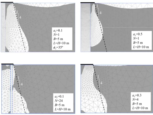
between compressive (positive) and extensive (negative) radial or horizontal strains is shown in Figure 3 for several cases, which were numerically simulated in Castro [13]. Figure 3 shows that the boundary between compressive and extensive horizontal strains is approximately at a slope of 4V:1H from the base of the footing, which happens to be the same as the assumed vertical stress distribution slope.

The footing is also assumed to be at the ground level, yet it will be usually embedded into the ground, which may be considered as an extra safety or later modified by an embedment correction factor.

2.4 Boundary conditions and material properties

The solution is developed for a horizontal slice at a depth z (Figure 4), and shear stresses between slices at different depths are neglected. The overall behaviour is obtained by means of addition of the solution, i.e. vertical deformation, at different depths. An average vertical stress, pa(z), is applied on each slice and is distributed

between soil and column. Average values of the vertical stress on the soil, _zs, and on the column, _zc, are used in the development of the analytical solution. The vertical strain at each horizontal slice, εz, is assumed as uniform, which is an acceptable

approximation because the load is applied on a rigid footing.

The boundary condition on the left-hand side (Figure 4) is the axis of symmetry and on the right-hand side, the radial strain is assumed as zero (εr=0), as explained above and

shown in Figure 3. It is worth noting that this boundary condition (εr=0) allows for a

horizontal displacement radially outwards, which means that there is not a full lateral confinement and the vertical strain is higher than for the “unit cell” case, where the lateral displacement at the outer boundary is restrained (e.g. Pulko et al. [2]). The radial distance, at which this boundary condition has to be applied, coincides with the lateral extension of the loaded area, rl(z), which varies with depth as explained in Figure 2.

of the column, Ac, is constant and the loaded area, Al, increases with depth. The area of the column is 2 , 2 ₄ 4 _{c ceq} c N d d

A    , where N is the number of columns in the group, and the subscript “eq” refers to the central equivalent column. So, similarly to Eq. (1), the area replacement ratio is given by

 

_

_{ }

_

Soil is assumed as elastic (Es, νs) but plastic strains are also considered in the column

using the Mohr-Coulomb yield criterion and a non-associated flow rule, with a constant dilatancy angle (Ec, νc, c, c).

The accuracy of the above simplifying assumptions will be evaluated in Section 5, comparing the results of the analytical model with numerical analyses.

3. ANALYTICAL SOLUTION

3.1 Elastic case

In a first step, elastic behaviour is assumed for the soil and the column. As previously mentioned, only a horizontal slice at a depth z of the unit cell is analysed (Figure 4). A horizontal slice of the column is a vertical solid cylinder subjected to a vertical uniform pressure _zc and a radial pressure rc at its lateral wall, i.e. it is subjected to a triaxial

                     rc z c c c c c c rc zc G G         2 2 (3)

Radial and hoop (circumferential) stresses are the same and constant within the column. Therefore, εrc=εθc=-sr/rc, where sr is the radial displacement at the soil/column interface,

which is positive radially outwards. Compressive stresses and strains are considered positive and Lamé's elastic constants are used for convenience (  G2 













The surrounding soil is a cylinder with a central cylindrical cavity, subjected to a vertical uniform pressure_zs, a radial pressure _rs at the cavity wall (soil/column interface) and a null radial strain (εr=0) at the external boundary (r=rl). Its solution is

derived in detail in Appendix I and is equal to





The stresses in Eqs. (3) and (4) correspond to stress increments produced by the applied load, pa. Compatibility of deformation at the soil/column interface in the horizontal

direction gives εrc=εθc=-εθs. Imposing radial equilibrium at the soil/column interface

(_rc_rs), the relationship between horizontal and vertical strains is obtained





s F a 

_  1

2 * ₍₅₎



 



To get the vertical strain, the condition of vertical equilibrium to soil and column is imposed.





Then, the vertical strain may be expressed as a function of an equivalent elastic modulus

e ml a z _E p   (8)

where the equivalent elastic modulus is

















and Em is the confined (oedometric) elastic modulus. The first and second terms in Eq.

(9) are the weighted values of the soil and column moduli, respectively.

Vertical and horizontal stresses can be determined substituting Eqs. (8) and (5) into Eq. (3) for the column and into Eq. (4) for the soil.

3.2 Plastic column

A key issue to correctly capture stone column behaviour is considering its yielding, which can be adequately modelled with the Mohr-Coulomb yielding criterion and a non-associated flow rule for the plastic strains, with a constant dilatancy angle

ac c c zc rc _K    _   sin 1 sin 1 (10) c c c p rc p zc _K      _     sin 1 sin 1 2 (11)

Stone column material is usually dense and granular with a negligible cohesion.

As for the elastic case, the column is assumed to be in compressive triaxial condition, and then, major principal stress direction is vertical. Now, column strains have an elastic part (Eq. 3) and another plastic (Eq. 11). Superscript "p" is used here to denote the plastic component. Combining those two components, the stress-strain relationship is:                    rc z c ac ac c E rc zc K K K K C       2 1 (12)

where CE is the following constant of the column, which has units of stiffness:





The column constant CE gives an idea of the importance of the elastic strains in the

column during its plastic deformation [22]. If the elastic strains are disregarded, 1/CE=0.

Now, in the elastic-plastic analysis, the effective stresses in the yield condition (Eq. 10) have to include also the initial stresses, existing before load application. Assuming an initial geostatic stress state, given by the effective unit weight of soil and column, γ’s

effective stresses are i zs s i rc i rs c i zc s i zs K z z , 0 , , , , ' '            (14)

Subscript "i" is used here to denote initial (prior to loading) stresses. Initially, the column is in an elastic state, because K_0s K_ac always, but the applied load, pa, may

cause column yielding. The value of the applied load that causes column yielding, y a p , may be obtained using Eq. (10)

ac y zc c y rc s s y zc y rc _K z z K       , , 0 , , ' '       (15)

where the subscript "y" refers to column yielding and the stress increments (denoted as ) are due to load application and may be obtained using Eqs. (3), (5) and (8). Substituting those equations in Eq. (15), y

a p is obtained. Yz py a  (16) where

























So, the applied load may be divided into the yielding load and the plastic increment

load, p a y a a p p p   .

procedure as for the elastic case, but replacing Eq. (3) by Eq. (12) to account for column elasto-plastic behaviour. Now, the relationship between horizontal and vertical strains is

z s K  _ * 2  (18) where









Imposing the condition of vertical equilibrium to soil and column, the vertical strain is

p ml p a z _E p   (20) where p ml

E is an equivalent modulus for the plastic increment









As for the elastic case, the vertical stresses and the radial displacement at the soil/column interface may be obtained substituting Eqs. (20) and (18) in Eqs. (4) and (12).

3.3 Solution

expressed as p ml p a e ml y a z y a a e ml a z y a a E p E p p p E p p p            If If (23)

To get the footing settlement, sz, the soil profile beneath the footing has to be divided

into several slices of finite thickness, Δt. The vertical deformation of each slice is approximate by the vertical strain at the centre of each slice. The addition of the vertical deformation of all of the slices gives the surface settlement

i i i z z t s 



To clarify the calculation procedure, an example is presented in the next section. The solution may be easily implemented in a spreadsheet or any programming language; an example is shown in Appendix II.

4. CALCULATION EXAMPLE

In this example, the soil profile is simplified to only one homogeneous soil layer of thickness H=10 m. The elastic properties of soil and column are Poisson's ratios of νs=νc=0.33 and Young's moduli of Es=2 MPa and Ec=30 MPa, respectively. That means

a modular ratio of 15. The friction and dilatancy angles for the column material are assumed as ϕc=45º and ψc=10º, respectively. For the sake of simplicity, the ground

water level is at the surface and the unit weights of soil and column are γs=γc=20 kN/m3,

pressure at rest of the soil is set equal to K0s=0.6, disregarding installation effects [18].

The foundation to be studied is a rough rigid square footing of side length B=5 m under a vertical pressure of pa=50 kPa. The soil beneath the footing is improved with 4 stone

columns, whose diameter is dc=0.9 m. So, the total column area is Ac=2 m2, and divided

by the footing area, Al=25 m2, gives the area replacement ratio at the base of the footing

ar(0)=10%. As shown in [12,13], the number of columns is not relevant if ar is kept

constant.

The square footing (B=5 m) is converted to a circular footing of same area. Therefore, its diameter is D2 B=5.64 m. In some practical situations, the diameter of the equivalent circular footing is directly taken as the side length of the square footing. The 4 columns are also converted to a central equivalent column. Its diameter gives the same total column area, d_c,eq Nd_c=1.8 m. If the columns, and consequently the equivalent central column, are assumed to reach a rigid substratum (end-bearing columns), their length is L=H=10 m.

As an example, the soil and the equivalent column are divided into 5 horizontal slices of same thickness, Δt=2 m. For this case, dividing the soil into 5 slices is accurate enough. No further comments are provided on the necessary number of horizontal slices as it is similar to other settlement calculations and depends on the natural layering of the soil. The applied vertical stress and the area replacement ratio at the centre of each horizontal slice are calculated using Eqs. (1) and (2). The results are shown in Table 1. Eqs. (9)

and (21) are used to get the equivalent moduli for the elastic and plastic cases, e ml E and p

ml

E , respectively. They are slightly different for each horizontal slice because they depend on the area replacement ratio. Next, the yielding load, y

a

p , is obtained with Eq. (16). The vertical strain at the centre of each horizontal slice, εz, is given by Eq. (23).

Finally, multiplying the slice thickness (2 m) by the vertical strains gives the deformation of each slice, szi, and the addition of the deformation of the 5 slices is the

footing settlement, sz=70 mm (Table 1).

5. VALIDATION AND PARAMETRIC ANALYSES

Using the previous calculation example as a reference case, parametric studies were carried out varying several properties. The calculation example and their parametric variations were also compared with numerical analyses to validate the accuracy of the analytical solution. The finite element method was used for the numerical simulations. Similarly to Castro [13], the codes Plaxis 3D 2012 [23] and Plaxis 2D 2012 [24] were used for the full 3D models and the simplified 2D axisymmetric models, respectively. The numerical models for the calculation example are shown in Figure 5. The results of the full 3D and the simplified 2D models are very similar [13]. So, for the sake of simplicity, only the results of the simplified 2D model are shown unless otherwise stated. The soil and column properties in the numerical model are the same as those used for the analytical solution.

5.1 Calculation example

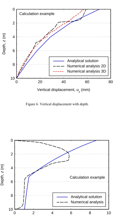
The footing settlement calculated in the previous section (sz=70 mm) is compared with

the footing settlement computed numerically, 59 and 57 mm, using the 2D and 3D models, respectively. The small difference between the 2D and 3D models is at least partly caused by the higher order of the elements used in the 2D model [13]. Although the analytical solution slightly overpredicts the settlement as explained below, it captures well the variation with depth (Figure 6). In the numerical models, the vertical line cross section corresponds to the centre of the footing, which means that it is in the column for the 2D model and in the soil for the 3D model. The oscillation at 2 m depth for the 2D model is caused by a shear band in the column (e.g. Pulko et al. [2]).

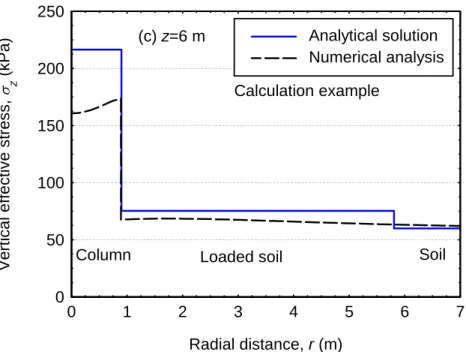
To further analyse the calculation example, the horizontal displacements at the soil/column interface are compared in Figure 7. The comparison is only possible with the 2D model because in the 3D model, there are 4 columns instead of the central equivalent column and the results are not comparable. Above roughly z=5 m, the horizontal displacements are significant, while below that depth, they are much lower. That is caused by the plastic strains in the column in the upper 5 m, while in the lower part, the column remains elastic. The analytical solution properly reproduces the horizontal displacements but for the upper (z=0) and lower (z=10 m) boundaries, which are rough (src=0) in the numerical model. Those differences in the boundary conditions

explain part of the difference in the settlement. Numerical simulations in the 2D model were performed using smooth upper and lower boundaries and the settlement increased from sz=59 mm to 61 mm. So, there is still a difference between the numerical model

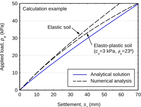
for the analytical solution (4V:1H) (Figure 2), as shown in the following.

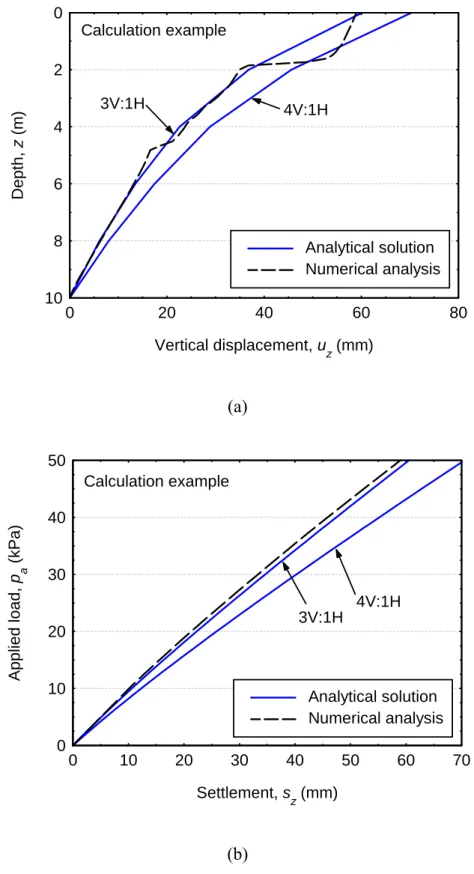
The vertical stresses, including the initial geostatic stress, are plotted at several depths in Figure 8. The assumed distribution of the vertical stress (Figure 2) is obviously a simplification, and in the numerical analyses there is not an abrupt distinction between loaded or not-loaded soil. However, the stress distribution between soil and column is well captured by the analytical solution and the general agreement is good. For this calculation example, the stress distribution assumed in the analytical solution (4V:1H) slightly overpredicts the vertical stresses, and consequently the vertical strains, particularly for z>B (e.g. Figure 8c). A 3V:1H distribution of the vertical load gives a better approximation and matches nearly perfectly the surface settlement (Figure 9). It is worth noting that a 4H:1V distribution is kept for the external boundary condition (εr=0). In the following, as an estimation on the safe side, the 4H:1V distribution for

both the vertical load and the external boundary condition is used if not otherwise stated.

5.2 Influence of soil yielding

The analytical solution assumes an elastic behaviour for the soil. For spread loadings and the unit cell model, the soil reaches its maximum strength only near the column and for high load levels. Consequently, assuming an elastic behaviour for the soil gives good settlement predictions for the unit cell model (e.g. [2]). However, the influence of soil plastic deformations for small groups of columns is more significant (e.g. [13]). To evaluate that influence, numerical analyses were performed. As an example, Figure 10

shows the load-settlement curves of the calculation example but including the numerical simulation with an elasto-plastic behaviour of the soil. The Mohr-Coulomb yield criterion and a non-associated flow rule, with a constant dilatancy angle were used for both soil and column. A low strength (s=23º, cs=3 kPa) and a non-dilatant behaviour

(s=0) were chosen for the soil. Obviously, plastic strains in the soil increase the

settlement but for low vertical loads (pa<20 kPa for the calculation example). For high

loads, plastic strains in the soil notably increase the settlement; ultimately, the bearing pressure is reached. Nevertheless, the proposed analytical solution is just for serviceability limit states, where soil yielding should be limited. For the calculation example and a service pressure around pa=50 kPa, the settlement overestimation

provided by the assumption of a 4V:1H distribution of the vertical load is compensated by the increase in the settlement that is caused by the soil plastic strains (Figure 10).

5.3 Floating columns

So far, only end-bearing columns have been considered, but the analytical solution is also applicable to floating columns, whose length is equal or higher than critical (L≥2B). Using the calculation example as a starting point, the soft soil layer thickness, H, was increased from 10 m to 40 m, while keeping the column length equal to the critical length (L=10 m). The case with columns (improved soil) and the case without columns (unimproved soil) were simulated, and, in both cases the footing settlement (sz and sz0, respectively) increases with H (Figure 11). The settlement increase beyond H=40 m=8B is small. For example, the settlement for a homogeneous elastic half-space without columns is around 96 mm.

The settlement reduction factor achieved with the improvement, which is defined as the coefficient between the settlement with columns and without columns, β=sz/sz0, does not notably change beyond the critical length (Figure 11) [12,13]. Therefore, the settlement reduction factor of floating columns whose length is equal or higher than critical (L≥2B) may be estimated studying those columns as if they were end-bearing columns. To get the settlement reduction factor, the settlement with columns is obtained using the proposed solution and the settlement without columns may be estimated also analytically using any conventional method (e.g. [25]). In some cases, assuming L≥2B may not be realistic, and then, the proposed solution is not applicable.

5.4 Influence of area replacement ratio

In the calculation example, the area replacement ratio at the base of the footing is low, namely ar(0)=10%, and therefore, the footing settlement is reduced by a small amount

(Figure 11). If a further reduction of the settlement is required, ar may be increased.

Figure 12 compares the footing settlement for several values of ar. The settlement

predicted by the proposed analytical solution assuming a 3V:1H load distribution matches very well the settlement computed numerically, while the settlement predicted by the proposed analytical solution assuming a 4V:1H load distribution gives a good estimation on the safe side.

5.5 Influence of footing width

the loaded area increases. However, as the factor D/H increases, the lateral confinement of the columns also increases and the settlement tends to an asymptotic value that corresponds to the “unit cell” model (full lateral confinement). As for previous cases, the analytical solution gives a conservative estimation of the computed settlement for a 4V:1H load distribution (Figure 13a), while a good matching is achieved using a 3V:1H distribution (Figure 13b).

For high values of D/H, e.g. higher than 1 for ar=30%, the lateral confinement is high

and the agreement between the proposed solution and the numerical analyses is worse because the hypothesis about the location of the external boundary where εr=0 is no

longer valid. Under high lateral confinement, i.e. high values of D/H, there is not a spreading of the external boundary and that boundary is nearly a vertical line from the edge of the footing (e.g. Figure 14). That means that the proposed solution has been developed for columns beneath footings or pads, and consequently, the solution and its hypotheses are valid for those cases but not for rafts or large loaded areas.

5.6 Influence of soil and column properties

To complete the parametric study and verify that the proposed analytical solution is able to accurately predict the footing settlement for the common range of problem parameters, the soil and column properties were also varied. Firstly, the column strength, namely the friction angle, was varied from 35º up to 50º. The dilatancy angle of the column was also varied accordingly, from 0º up to 15º. The footing settlement evidently decreases as the column friction and dilatancy angles increase (Figure 15),

because the column yields later and the plastic strains are less important. The analytical solution assuming a 4V:1H load distribution gives a good estimation on the safe side; only for high area replacement ratios and very low column strengths (e.g. ar=50%,

c=35º, c=0), the analytical solution gives slightly higher settlement.

Secondly, the soil and column Young’s moduli were varied. For the same modular ratio, Ec/Es, the results of both parametric analyses are the same if the footing settlement is

expressed in terms of the settlement reduction factor, β (Figure 16). The results confirm that the proposed analytical solution gives a good estimation on the safe side. The agreement between the analytical solution and the numerical analyses is better for high values of ar and Ec/Es, because the load distribution is closer to 4V:1H. On the contrary,

for low ar or Ec/Es, the vertical load spreads out on a wider area and the load distribution

slope of 4V:1H assumed for the analytical solution gives conservative values, i.e. overestimates β. Ultimately, for ar=0% or Ec/Es=1, the analytical solution would

significantly overestimate , if a 4H:1V load distribution slope is assumed instead of a more realistic slope of 2H:1V for the case of no improvement.

5.7 Comparison with published experimental measurements

To fully validate the proposed analytical solution, a comparison with experimental measurements is here presented. The set of high-quality laboratory experiments performed by Sivakumar et al. [26] were used because of the detailed information provided. Sivakumar et al. [26] performed model tests on soft soil samples, 300 mm in

diameters, namely dc=40, 50 and 60 mm. A 60 mm diameter footing was resting on top

of the column and subjected to foundation loading under drained conditions. The resulting area replacement ratios are ar=44, 69 and 100%, respectively. Speswhite

kaolin and crushed basalt were used to model the soft soil and the stone column. Their properties may be found in Black et al. [9]. Those relevant for the analytical solution are Es= 4 MPa, Ec=30 MPa, ϕc=43º. Common values were assumed for other parameters

that are not provided, νc=νs=0.33 and ψc=10º. The soil samples were isotropically

consolidated (K0=1) to 50 kPa. That is the initial stress state for this case (Eq. 14). The

soil and column weight were neglected. The columns were fully penetrating (L=400 mm) but the deformation below 2D=120 mm was assumed to be small, and therefore, for the analytical solution the column length was input as 120 mm.

Although there is some scatter in the laboratory data, the predicted settlement by the analytical solution matches reasonably well the laboratory measurements for design footing pressures (Figure 17). For higher pressures, e.g. pa>60-100 kPa, the

experimental load-displacement curves bend towards the bearing pressure because of soil plastic deformation.

5.8 Limit of the applied load

As shown in Section 5.2 and Figure 17, the proposed solution is only valid for low or moderate applied loads that do not generate significant plastic strains in the natural soft soil. An exhaustive analysis of the soil plastic strains is beyond the scope of the paper, but further information and some comments are presented here to provide some

guidance on the limit of the applied load when using the proposed solution.

For the calculation example, the proposed solution gives conservative settlements for loads not exceeding 50 kPa (Figure 10). This limit increases with the soil strength, footing diameter and area replacement ratio. As an example, Figure 18 shows the settlement predicted by the analytical solution and the numerical analysis, considering soil plastic strains (s=23º, cs=3 kPa) for different area replacement ratios. When the

predicted values by the analytical solution and the numerical analysis coincide, that is considered the limit of the applied load to be used in the analytical solution. The limit load for the calculation example, i.e. ar=10%, is 50 kPa, but this value increases up to

75 kPa for ar=60% and up to 100 kPa for ar=80%. Those values are higher for higher

soil strengths and footing diameters.

In the comparison with the laboratory measurements presented in the previous section (Figure 17), the limit load is between 60 and 100 kPa, depending on ar and the scatter of

the laboratory results. Although the footing diameter is small, the limit load is similar to the previous calculation example because of the higher soil strength.

In summary, for common situations (footing diameter, soil strength and ar), the limit of

CONCLUSIONS

A new approximate solution has been developed to study the settlement of rigid footings resting on a soft soil improved by groups of stone columns. The solution development is fully analytical, imposing equilibrium of stresses and compatibility of deformations. Some simplifying assumptions are necessary, such as:

 Groups of columns are converted to equivalent single columns with the same cross-sectional area. So, the problem becomes axially symmetric.

 Applied load distributes with depth at a 4V:1H slope. For some cases, a 3V:1H load distribution gives a closer approximation.

 Columns reach a rigid substratum or their length (L) is higher than critical (≈2B).  Soil profile is divided into slices that are independently analysed.

 Plastic strains in the soil are not considered.  Foundation loading is under drained conditions.

These simplifying assumptions impose some limitations to the analytical solution. The solution is not directly applicable to large loaded areas or stratified soils because the load distribution slope changes. Additionally, the solution is not applicable to those cases where the column does not reach a rigid substratum and it is not realistic to assume L≥2B. The solution is only valid for low to moderate foundation loads (lower than 50-100 kPa for common cases) because plastic strains in the soil are not considered.

The solution may be implemented in a spreadsheet or any programming language. A simplified calculation example and the corresponding Matlab code are presented.

The analytical solution predicts footing settlements that agree well with numerical analyses and are usually on the safe side for most cases. Good agreement is also found for vertical displacements, vertical stresses and horizontal displacements at the soil/column interface. Additionally, the solution compares well with a small scale laboratory test available in literature, which confirms the validity of the solution and its hypotheses. So, the proposed solution is an analytical and accurate tool for the design of groups of stone columns beneath rigid footings.

REFERENCES

[1] Balaam NP, Booker JR (1985) Effect of stone column yield on settlement of rigid foundations in stabilized clay. Int J Num Anal Meth Geomech 9(4):331-351

[2] Pulko B, Majes B, Logar J (2011) Geosynthetic-encased stone columns: Analytical calculation model. Geotext Geomembranes 29(1):29-39

[3] Castro J, Sagaseta C (2009) Consolidation around stone columns. Influence of column deformation. Int J Numer Anal Meth Geomech 33(7):851-877

[4] Barksdale RT, Bachus RC (1983) Design and construction of stone columns. Report FHWA/RD-83/026. Springfield: Nat Tech Information Service

[5] Watts KS, Johnson D, Wood LA, Saadi A (2000) An instrumented trial of vibro ground treatment supporting strip foundations in a variable fill. Géotechnique 50(6):699-708

[6] Wood DM, Hu W, Nash DFT (2000) Group effects in stone column foundations: model tests. Géotechnique 50(6):689-698

[7] McKelvey D, Sivakumar V, Bell A, Graham J (2004) Modelling vibrated stone columns in soft clay. Proc ICE - Geotech Eng 157(3):137-149

[8] Wehr J (2004) Stone columns – single columns and group behaviour. Proc 5 Int Conf Ground Improvement Tech, Kuala Lumpur, pp. 329-340

[9] Black JA, Sivakumar V, Bell A (2011) The settlement performance of stone column foundations. Géotechnique 61(11):909-922

[10] Shahu J, Reddy Y (2011) Clayey Soil Reinforced with Stone Column Group: Model Tests and Analyses. J Geotech Geoenviron Eng 137(12):1265–1274

[11] Killeen M (2012) Numerical modelling of small groups of stone columns. PhD Thesis. National University of Ireland, Galway

[12] Ng KS (2013) Numerical study of floating stone columns. PhD Thesis. National University of Singapore

[13] Castro J (2014) Numerical modelling of stone columns beneath a rigid footing. Comput Geotech 60:77-87.

[14] Priebe HJ (1995) Design of vibro replacement. Ground Eng 28(10):31-37

[15] Stuedlein AW, Holtz RD (2014) Displacement of spread footings on aggregate pier reinforced clay. J Geotech Geoenviron Eng 140(1):36-45

[16] Sehn AL, Blackburn JT (2008) Predicting performance of aggregate piers. Proc 23rd Central Pennsylvania Geotechnical Conf, Central Pennsylvania ASCE Geotechnical Group, Hershey

[17] Ambily AP, Gandhi SR (2007) Behavior of stone columns based on experimental and FEM analysis. J Geotech Geoenviron Eng 133(4):405-415

[18] Castro J, Karstunen M (2010) Numerical simulations of stone column installation. Can Geotech J 47(10):1127-1138

[19] Mitchell JK, Huber TR (1985) Performance of a stone column foundation. J Geotech Eng 11(2):205-223

[20] Schweiger HF (1989) Finite element analysis of stone column reinforced foundations. PhD Thesis, University of Wales, Swansea

[21] Tomlinson M, Woodward J (2008) Pile design and construction practice. 5th _Ed. Abingdon: Taylor & Francis

[22] Castro J, Sagaseta C (2013) Influence of elastic strains during plastic deformation of encased stone columns. Geotext Geomembranes 37:45-53

[23] Brinkgreve RBJ, Engin E, Swolfs WM (2012) Plaxis 3D 2012 Manual. Plaxis bv, the Netherlands

[24] Brinkgreve RBJ, Engin E, Swolfs WM (2012) Plaxis 2D 2012 Manual. Plaxis bv, the Netherlands

[25] Mayne PW, Poulos HG (1999) Approximate displacement influence factors for elastic shallow foundations. J Geotech Geoenviron Eng 125(6):453-460

[26] Sivakumar V, Jeludine DKNM, Bell A, Glynn DT, Mackinnon, P (2011) The pressure distribution along stone columns in soft clay under consolidation and foundation loading. Géotechnique 61(7):613-620

[27] Balaam NP, Booker JR (1981) Analysis of rigid rafts supported by granular piles. Int J Num Anal Meth Geomech 5:379-403

APPENDIX I: SOLUTION FOR THE SOIL HOLLOW CYLINDER

The soil surrounding the column is a hollow cylinder, subjected to a vertical uniform pressure_zs, a radial internal pressure _rs at the soil/column interface (r=rc) and a null

radial strain (εr=0) at the external boundary (r=rl) (Figure 4). The solution is obtained by

superposition of a state A of confined vertical compression and a state B in plane strain conditions (e.g. [27]). In state A, there is only vertical deformation, εz, and in state B,

there are only horizontal deformations, εr and εθ. The solution for state A is

                    s z s s s A rs A zs G        2 0 0 2 , , (A.1)

where εθs is the hoop strain at the soil/column interface (r=rc) and is related to the radial

displacement at the soil/column interface, εθs=sr/rc.

The solution for state B starts with the displacement field for a hollow cylinder in plane strain conditions and axial symmetry (uθ=0):

r B Ar

u_r   (A.2)

where A and B are constants that satisfy the boundary conditions. From the displacement field (Eq. A.2), the strains may be calculated

2 2 r B A r u r B A r u r r r            (A.3)

The stresses are













and the boundary conditions are









Applying the boundary conditions (Eq. A.5) to Eqs. (A.3) and (A.4), the constants A and B and the solution for state B are calculated.





The final solution is obtained by superposition of states A (Eq. A.1) and B (Eq. A.6).





APPENDIX II: CODE FOR THE ANALYTICAL SOLUTION

The analytical solution may be implemented in a spreadsheet or any programming language. This appendix shows an example of code in Matlab to get the footing settlement. The data of the calculation example in Section 4 are here used.

% Units: Length (m), Stiffness and applied pressure (kPa), Unit weight (kN/m3) % Geometry data

% Square footing

B=5;

%Equivalent circular footing

D=2/sqrt(pi)*B;

% Number of columns, diameter and length (end-bearing columns)

N=4; dc=0.9; L=10;

% Divide soil and column into n slices

n=5; % Soil properties Es=2000; mus=0.33; gammas=10; K0s=0.6; % Column properties Ec=30000; muc=0.33; gammac=10; fic=45*pi/180; chic=10*pi/180; % Applied load pa0=50; % Intermediate parameters deltat=L/n; vz=linspace(0+deltat/2, L-deltat/2, n); Ems=Es*(1-mus)/((1+mus)*(1-2*mus)); Gs=Es/(2*(1+mus)); lamdas=Ems-2*Gs; Emc=Ec*(1-muc)/((1+muc)*(1-2*muc)); Gc=Ec/(2*(1+muc)); lamdac=Emc-2*Gc; Kac=(1-sin(fic))/(1+sin(fic)); Kchic=(1-sin(chic))/(1+sin(chic)); CE=(3*lamdac+2*Gc)/(1+2*Kac*Kchic+lamdac/Gc*(1-Kac-Kchic+Kac*Kchic)); sz=0;

% Deformation of each slice

for i=1: n z=vz(i); ar=N*dc*dc/(D+z/2)^2; pa=pa0*D*D/(D+z/2)^2; Fstar=(lamdac-lamdas)/(ar*(lamdac+lamdas+Gc+Gs)+(lamdac+Gc-Gs)); Emle=ar*Emc+(1-ar)*Ems+Fstar*ar*(lamdas*(1-ar)-lamdac*(1+ar));

Y=(K0s*gammas-Kac*gammac)*Emle/(Gc*(2*Kac+Fstar*(1+ar))-lamdac*(1-Kac)*(1-Fstar*(1+ar))); pay=Y*z; if pa>pay pap=pa-pay; ez=pay/Emle+pap/Emlp; else ez=pa/Emle; end

% Addition of the deformation of each slice

sz=sz+ez*deltat*1000;

end

% Total settlement in mm

TABLE CAPTIONS

FIGURE CAPTIONS

Figure 1. Modelling of a group of stone columns beneath a rigid footing: (a) Real geometry ; (b) Equivalent concentric rings ; (c) Homogenization technique ; (d) Equivalent central column.

Figure 2. Stress distribution beneath the footing: (a) End-bearing columns; (b) Floating columns.

Figure 3. Limit between extensive (in white) and compressive (in grey) horizontal strains.

Figure 4. Analytical model.

Figure 5. Numerical models [13]. Calculation example: (a) 3D model; (b) Simplified 2D model.

Figure 6. Vertical displacement with depth.

Figure 7. Horizontal displacements at the soil/column interface. Figure 8. Vertical stresses at several depths.

Figure 9. Different load distributions: (a) Vertical displacement with depth; (b) Load-settlement curve.

Figure 10. Influence of soil plastic strains.

Figure 11. Influence of soil layer thickness. Numerical analyses. Figure 12. Influence of area replacement ratio.

Figure 13. Influence of footing width: (a) 4V:1H load distribution; (b) 3V:1H load distribution.

Figure 14. Limit between extensive (in white) and compressive (in grey) radial strains (D/H=2).

Figure 15. Influence of column strength.

Figure 16. Influence of soil and column stiffnesses.

Table 1. Calculation example.

Depth pa ar E_mle E_mlp p_ay εz szi

(m) (kPa) (%) (kPa) (kPa) (kPa) (%) (mm)

1 42.2 8.4 5,373 3,234 5.6 1.24 25 3 31.2 6.2 4,746 3,140 14.6 0.84 17 5 24.0 4.8 4,335 3,086 22.1 0.57 11 7 19.0 3.8 4,051 3,054 28.8 0.47 9 9 15.5 3.1 3,848 3,032 35.1 0.40 8 Total 70

Improved properties

(a) (b) (c) (d)

Figure 1. Modelling of a group of stone columns beneath a rigid footing: (a) Real geometry ; (b) Equivalent concentric rings ; (c) Homogenization technique ; (d) Equivalent central column.

p

(0)

B

z

p

(z)

ar=0.1 N=1 B=5 m L=H=10 m ϕc=35º 4 1 ₄ 1 ar=0.5 N=1 B=5 m L=H=10 m ar=0.1 N=24 B=5 m L=H=10 m 4 1 ar=0.3 N=4 B=5 m L=H=10 m 4 1

Figure 3. Limit between extensive (in white) and compressive (in grey) horizontal strains.

L

Columns Rough rigid square footing Soil Applied pressure Roller  vertical  boundaries Fixed bottom  boundary 10 m 15 m 15 m (a) Applied pressure Column Soil Rough rigid circular footing Fixed bottom 

boundary Roller vertical _boundaries Axis of symmetry

(b)

0 2 4 6 8 10 0 20 40 60 80 Analytical solution Numerical analysis 2D Numerical analysis 3D Calculation example Vertical displacement, u z (mm) Depth, z (m )

Figure 6. Vertical displacement with depth.

0 2 4 6 8 10 0 2 4 6 8 10 Analytical solution Numerical analysis Calculation example

Horizontal displacement at the soil/column interface, s

rc (mm)

Depth,

z

(m

)

0 50 100 150 200 0 1 2 3 4 5 Analytical solution Numerical analysis (a) z=2 m Soil Loaded soil Column Calculation example Radial distance, r (m) Ve

rtical effective stress

,  z (k P a ) 0 50 100 150 200 0 1 2 3 4 5 Analytical solution Numerical analysis (b) z=4 m Soil Loaded soil Column Calculation example Radial distance, r (m) Ve

rtical effective stress

,  z (k P a )

0 50 100 150 200 250 0 1 2 3 4 5 6 7 Analytical solution Numerical analysis (c) z=6 m Soil Loaded soil Column Calculation example Radial distance, r (m) Ve

rtical effective stress

,  z (k P a )

0 2 4 6 8 10 0 20 40 60 80 Analytical solution Numerical analysis 3V:1H _4V:1H Calculation example Vertical displacement, u z (mm) Depth, z (m ) (a) 0 10 20 30 40 50 0 10 20 30 40 50 60 70 Analytical solution Numerical analysis Calculation example 3V:1H 4V:1H Settlement, s_z (mm) Applied load, p a (kPa) (b)

0 10 20 30 40 50 0 10 20 30 40 50 60 70 Analytical solution Numerical analysis Calculation example Elastic soil Elasto-plastic soil (c s=3 kPa, s=23º) Settlement, s z (mm) Applied load, p a (kPa)

Figure 10. Influence of soil plastic strains.

0 20 40 60 80 100 10 20 30 400 0.4 0.8 1.2 1.6 2.0 s_z0 s_z  Calculation example L=2B= 10 m

Soil layer thickness, H (m)

Settlem ent (mm ) Settlemen t reduction factor,  = s z /s z 0

0 20 40 60 80 100 0 20 40 60 80 100 Analytical solution Numerical analyses 4V:1H 3V:1H Calculation example

Area replacement ratio, a

r (%) Settlem ent, s z (m m)

0 20 40 60 80 100 120 0 0.5 1.0 1.5 2.0 Analytical solution (4V:1H) Numerical analyses a_r=50% a_r=30% a_r=10% Calculation example L=H= 10 m

Normalised footing width, D/H

Settlement, s z (mm) (a) 0 20 40 60 80 100 120 0 0.5 1.0 1.5 2.0 Analytical solution (3V:1H) Numerical analyses a r=50% a r=30% a_r=10% Calculation example L=H= 10 m

Normalised footing width, D/H

Settlement,

s z

(mm)

(b)

ar=0.3 N=1 D=20 m L=H=10 m 4 1

Figure 14. Limit between extensive (in white) and compressive (in grey) radial strains (D/H=2).

0 20 40 60 80 100 35 40 45 50 0 5 10 15 Analytical solution Numerical analyses  c  c Calculation example a r=50% a r=30% a r=10%

Column friction and dilatancy angles, 

c and c (º)

Settlement,

s z

(mm

)

0 0.2 0.4 0.6 0.8 1.0 15 30 45 60 Analytical solution Numerical analyses Calculation example a_r=50% a r=30% a r=10% Modular ratio, E c / Es Settlem

ent reduction factor,



= s

z

/

s z0

Figure 16. Influence of soil and column stiffnesses.

0 50 100 150 200 0 0.5 1.0 1.5 D=40 mm D=50 mm D=60 mm 40 50 60 Analytical solution (D in mm) Laboratory tests (Sivakumar et al. [26]) Settlement, s z (mm) Applied load, p a (k P a )

0 20 40 60 80 100 0 20 40 60 80 100 Anal. solution Num. analysis 100 kPa 75 kPa p a=50 kPa Calculation example Elasto-plastic soil (c s=3 kPa ; s=23º)

Area replacement ratio, a

r (%) Settlem ent, s z (m m)