Computational Statistics & Data Analysis 00 (2016) 1–21
Journal
Logo
The joint role of trimming and constraints in robust estimation
for mixtures of Gaussian factor analyzers
Luis Angel Garc´ıa-Escudero
a, Alfonso Gordaliza
a, Francesca Greselin
b,
Salvatore Ingrassia
c, Agust´ın Mayo-Iscar
aaDepartment of Statistics and Operations Research and IMUVA, University of Valladolid (Spain) bDepartment of Statistics and Quantitative Methods, Milano-Bicocca University (Italy)
cDepartment of Economics and Business, University of Catania (Italy)
Abstract
Mixtures of Gaussian factors are powerful tools for modeling an unobserved heterogeneous population, offering - at the same time - dimension reduction and model-based clustering.The high prevalence of spurious solutions and the disturbing effects of outlying observations in maximum likelihood estimation may cause biased or misleading inferences. Restrictions for the component covari-ances are considered in order to avoid spurious solutions, and trimming is also adopted, to provide robustness against violations of the normality assumptions of the underlying latent factors. A detailed AECM algorithm for this new approach is presented. Simulation results and an application to the AIS dataset show the aim and effectiveness of the proposed methodology.
c
2015 Published by Elsevier Ltd.
Keywords: Constrained estimation, Factor Analyzers Modeling, Mixture Models, Model-Based Clustering,, Robust estimation.
1. Introduction and motivation
Factor analysis is an effective method of summarizing the variability between a number of correlated features, through a much smaller number of unobservable, hence named latent, factors. It originated from the consideration that, in many phenomena, several observed variables could be explained by a few unobserved ones. Under this approach, each single variable (among the p observed ones) is assumed to be a linear combination of d underlying common factors with an accompanying error term to account for that part of the variability which is unique to it (not in common with other variables). Ideally, d should be substantially smaller than p, to achieve parsimony.
Clearly, the effectiveness of this method is limited by its global linearity, as happens for principal components analysis. Hence, Ghahramani and Hilton (1997), Tipping and Bishop (1999) and McLachlan and Peel (2000a) solidly widened the applicability of these approaches by combining local models of Gaussian factors in the form of finite mixtures. The idea is to employ latent variables to perform dimensional reduction in each component, thus providing a statistical method which concurrently performs clustering and, within each cluster, local dimensionality reduction.
In the literature, error and factors are routinely assumed to have a Gaussian distribution because of their mathemat-ical and computational tractability: however, statistmathemat-ical methods which ignore departure from normality may cause
Email addresses:[email protected](Luis Angel Garc´ıa-Escudero),[email protected](Alfonso Gordaliza),
[email protected](Francesca Greselin),[email protected](
biased or misleading inferences. Moreover, it is well known that maximum likelihood estimation for mixtures often leads to ill-posed problems because of the unboundedness of the objective function to be maximized, which favors the appearance of non-interesting local maximizers and degenerate or spurious solutions.
The lack of robustness in mixture fitting arises whenever the sample contains a certain proportion of data that does not follow the underlying population model. Spurious solutions can even appear when ML estimation is applied to artificial data drawn from a given finite mixture model, i.e. without adding any kind of contamination. Hence, robust estimation is needed. Many contributions in this sense can be found in the literature: from the Mclust model with a noise component in Fraley and Raftery (1998), mixtures of t-distributions in McLachlan and Peel (2000), the trimmed likelihood mixture fitting method in Neykov et al. (2007), the trimmed ML estimation of contaminated mixtures in Gallegos and Ritter (2009), and the robust improper ML estimator introduced in Coretto and Hennig (2011), among many others. Some important applications in such fields as computer vision, pattern recognition, analysis of microarray gene expression data, or tomography suggest that more attention should be paid to robustness, because noise in the data sets may be frequent in all these fields of application.
Different types of constraints have been traditionally applied in Gaussian mixtures of factor analyzers, for instance, some authors propose taking a common (diagonal) error matrix (as for the Mixtures of Common Factor Analyzers, denoted by MCFA, in Baek et al., 2010) or imposing an isotropic error matrix (Bishop and Tipping, 1998). This strategy has proven to be effective in many cases, at the expenses of stronger distributional restrictions on the data. To avoid singularities and spurious solutions, under milder conditions, Greselin and Ingrassia (2015) recently proposed maximizing the likelihood by constraining the eigenvalues of the covariance matrices, following the previous work of Ingrassia (2004) and going back to Hathaway (1985). Furthermore, mixtures of t-analyzers have been considered (see McLachlan and Bean, 2005; Lin et al., 2014, and references therein) in an attempt to make the model less sensitive to outliers, but they, too, are not robust against very extreme outliers (Hennig, 2004).
The purpose of the present work is to introduce an estimating procedure for the mixture of Gaussian factor ana-lyzers that can resist the effect of outliers and avoid spurious local maximizers. The proposed constraints can also be used to take into account prior information about the scatter parameters.
Trimming has been shown to be a simple, powerful, flexible and computationally feasible way to provide robust-ness in many different statistical frameworks. The basic idea behind trimming here is the removal of a small proportion
αof observations whose values would be the most unlikely to occur if the fitted model were true. In this way, trimming avoids the problem of a small fraction of outlying observations exerting a harmful effect on the estimation. Incorpo-rating constraints into the mixture fitting estimation method moves the mathematical problem to a well-posed setting and hence minimizes the risk of incurring spurious solutions. Moreover, a correct statement of the problem allows the desired statistical properties for the estimators to be obtained, such as the existence and consistency results, as in Garc´ıa-Escudero et al. (2008).
The rest of the paper has been organized as follows. In Section 2,the notation is introduced and the main ideas
about Gaussian Mixtures of Factor Analyzers (hereafter denoted by MFA) are summarized. Then, in Section 3, the
trimmed likelihood for MFAis presented, and fairly extensive notes are provided concerning the EM algorithm, with
incorporated trimming and constrained estimation. In Section 4, the performance of the new procedureis discussed,
on the grounds of some numerical results obtained from simulated and real data. In particular, the bias and MSE
of robustly estimated model parameters for different cases of data contamination, are compared, using Monte Carlo
experiments.The application to the Australian Institute of Sports dataset shows how classification and factor analysis
can be developed using the new model. Section 5 contains concluding notes and provides ideas for further research.
2. Gaussian Mixtures of Factor Analyzers
The density of the p-dimensional random variable X of interest is modeled as a mixture of G multivariate normal densities in some unknown proportionsπ1, . . . πG, whenever each data point is taken to be a realization of the following density function:
f (x;θ)=
G
X
g=1
πgφp(x;µg,Σg) (1)
component meansµg, and the12G p(p+1) distinct elements of the component-covariance matricesΣg. MFA postulates a finite mixture of linear sub-models for the distribution of the full observation vector X, given the (unobservable) factors U. That is, MFA provides local dimensionality reduction by assuming that the distribution of the observation Xican be given as
Xi=µg+ΛgUig+eig with probability πg(g=1, . . . ,G) for i=1, . . . ,n, (2)
whereΛg is a p×d matrix of factor loadings, the factors U1g, . . . ,UngareN(0,Id) distributed independently of the
errors eig. The latter are independentlyN(0,Ψg) distributed, andΨgis a p×p diagonal matrix (g=1, . . . ,G). The
diagonality ofΨgis one of the key assumptions of factor analysis: the observed variables are independent given the factors. Note that the factor variables Uigmodel correlations between the elements of Xi, while the errors eigaccount for independent noise for Xi. We suppose that d <p, which means that d unobservable factors are jointly explaining
the p observable features of the statistical units. Under these assumptions, the mixture of factor analyzers model is given by (1), where the g-th component-covariance matrixΣghas the form
Σg=ΛgΛ′g+Ψg (g=1, . . . ,G). (3)
The parameter vectorθ=θMFA(p,d,G) now consists of the elements of the component meansµg, theΛg, and theΨg, along with the mixing proportionsπg(g=1, . . . ,G−1), on puttingπG=1−PGi=−11πg.
Note that, in the case of d>1, there is an infinity of choices forΛg, since model (2) is still satisfied if we replace
ΛgbyΛgH′, where H is any orthogonal matrix of order d. As d(d−1)/2 constraints are needed forΛgto be uniquely
defined, the number of free parameters for each component of the mixture is given by
pd+p−1
2d(d−1).
The following condition on p and d assures the desired parsimony:
[(p−d)2−(p+d)]>0.
3. Robust Mixtures of Factor Analyzers
In this section, the trimmed (Gaussian) mixtures of factor analyzers model (trimmed MFA) is presented and a feasible algorithm for its implementation is provided.
3.1. Problem statement
Let x ={x1,x2, . . . ,xn}be a given data set inRp. With the theoretical underlying model described in Section 3 in mind, a mixture of Gaussian factor components can be robustly fitted to this dataset x by maximizing a trimmed
mixture log-likelihood (see Neykov et al. 2007, Gallegos and Ritter 2009 and Garc´ıa-Escudero et al. 2014) defined as:
Ltrim=
n
X
i=1
ζ(xi) log
G
X
g=1
φp(xi;µg,Σg)πg
(4)
whereζ(·) is a 0-1 trimming indicator function that tells us whether observation xi is trimmed off: ζ(xi)=0, or not:
ζ(xi)=1 andΣg =ΛgΛ′g+Ψgas in (3). A fixed fractionαof observations can be unassigned by settingPn
i=1ζ(xi)= [n(1−α)] and, hence, the parameterαdenotes the trimming level.
Moreover, to avoid the unboundedness ofLtrim, constrained maximization of (4) is introduced. In more detail, with reference to the diagonal elements{ψgk}k=1,...,pof the noise matricesΨgfor g=1, . . . ,G, it is required that
The constant cnoiseis finite and such that cnoise≥1, to avoid the|Σg| →0 case. This constraint can be seen as an adaptation to MFA of those introduced in Ingrassia and Rocci (2007), Garc´ıa-Escudero et al. (2008), and is similar to the mild restrictions implemented for MFA in Greselin and Ingrassia (2015). They all go back to the seminal paper of Hathaway (1985). We will look for the maximization ofLtrimonΨgunder the given constraints: this setting leads to a well-defined maximization problem, and at the same time allows singularities to be discarded and the occurrence of spurious solutions to be reduced.
Our methodology also includes the possibility of controlling the relative variability of the norms of the p dimen-sional column vectors of the matricesΛg(for g=1, . . . ,G). If{ηk g}k=1,...,ddenotes the set of these norms, a second set of constraints applies on their values
ηk g1 ≤cload ηh g2 for every 1≤k,h≤d and 1≤g1,g2≤G. (6)
In fact, these types of constraints are not needed to avoid singularities in the target function, but they could be useful to achieve more sensible solutions.
Hereafter,Θcwill denote the constrained parameter space forθ={πg, µg,Ψg,Λg; g=1, . . . ,G}under the require-ments (5) and (6).
3.2. Algorithm
The maximization ofLtrimin (4) forθ ∈ Θcis not an easy task, obviously. We will give a feasible algorithm obtained by combining the Alternating Expectation-Conditional Maximization algorithm (AECM) for MFA with that (with trimming and constraints) introduced in Garc´ıa-Escudero et al. (2014) (see, also, Fritz et al., 2013).
As usual in the EM framework, each observation xiis associated with an unobserved state zi =(zi1, . . . ,ziG)′for
i =1, . . . ,n where zigis one or zero, depending on whether xidoes or does not belong to the g-th component. The component label vectors z1, . . . ,znare taken to be the realized values of the random vectors Z1, . . . ,Zn, where, for independent feature data, it is appropriate to assume that they are (unconditionally) multinomially distributed. i.e. Z1, . . . ,Zn ∼i.i.d. MultG(1;π1, ..., πG). The AECM is an extension of the EM, suggested by the factor structure of the model, which uses different specifications of missing data at each stage. The idea is to partition the vector of parametersθ = (θ1,θ2) in such a way thatLtrimis easy to be maximized for θ1 givenθ2 and viceversa, replacing the M-step by a number of computationally simpler conditional maximization (CM) steps. In more detail, in the first cycle we setθ1 ={πg,µg; g=1, . . . ,G}and the missing data are the unobserved group labels z=(z1, . . . ,zn)′; while in the second cycle we setθ2={Λg,Ψg; g=1, . . . ,G}and the missing data are the group labels z and the unobserved latent factors u =(u11, . . . ,unG)′. Hence, the application of the AECM algorithm consists of two cycles, and there is one E-step and one CM-step, alternatively consideringθ1 andθ2 in each cycle. A trimming step, to evaluate the trimming function, precedes each cycle. The trimming function has the role of discarding theα100% of observations with lowest contribution to the likelihood. Before describing the algorithm, we remark that the unobserved group labels Z are considered missing data in both cycles. Therefore, during the l-th iteration, z(lig+1/2)and z(lig+1)denote the conditional expectations at the first and second cycle, respectively.
The algorithm has to be run multiple times on the same dataset, with different starting values, to prevent the attainment of a local, rather than global, maximum log-likelihood. In each run it executes the following steps:
1 Initialization:
Each iteration begins by selecting initial values forθ(0)whereθ(0)=(π(0) g , µ
(0) g ,Λ(0)g ,Ψ
(0)
model (2) in group g as a regression of Xi with interceptµg, regression coefficients given byΛg, where the explanatory variables are the latent factors Uig, and with regression errors eig. Hence, we draw p+1 random independent observations from the d-variate standard Gaussian to fill a (p+1)×d matrix ug. Then we set
Λ(0)g = ((ug)′ug)−1(ug)′xg
c, where x g
c is obtained by centering the columns of the xg matrix. To provide a restricted random generation ofΨg, the (p+1)×p matrixεg = xgc −Λ(0)g ug is computed, and the diagonal elements of Ψ(0)g are set equal to the variances of the p columns of the εg matrix. After repeating this for
g=1, . . . ,G, if the obtained matricesΛ(0)g andΨ(0)g do not satisfy the required constraints (5) and (6), then the constrained maximizations described in step 2.4 must be applied. Finally, weightsπ(0)1 , ..., π(0)G in the interval (0,1) and summing up to 1 are randomly chosen.
2 Trimmed AECM steps:
The following steps 2.1–2.6. are alternatively executed until a maximum number of iterations, MaxIter, is reached. The implementation of trimming is related to the “concentration” steps applied in high-breakdown robust methods (Rousseeuw and Van Driessen, 1999). Trimming is performed before each E-step, while con-straints are enforced during the second cycle CM step.
2.1 First cycle. Trimming: Evaluate the n quantities
D(xi;θ(l))=
G
X
g=1
φp(xi;µg,ΛgΛ′g+Ψg)πg for i=1, . . . ,n
and sort them to obtain theirαquantile denoted by D([nα]). Notice that D(xi;θ(l)) is the contribution given from xito the overall likelihood. Now consider the set of indices I⊂ {1,2, ...,n}defined as
I=i : D(xi;θ(l))≥D ([nα]) .
Then set the trimming function asζ(xi)=1 for i∈I, andζ(xi)=0 otherwise. To update the parameters, only the observations with indices in I will be taken into account. In other words, the proportionαof observations with the smallest D(xi;θ(l)) valuesare tentatively discarded.
2.2 First cycle. E-step:
Hereθ1 = {πg,µg; g =1, . . . ,G}and the missing data are the unobserved group labels z=(z1, . . . ,zn)′. The E-step on the first cycle on the (l+1)-th iteration requires the calculation of
Q1
θ1;θ(l)
=Eθ(l)
h
n
X
i=1 ζ(xi)
G
X
g=1
Zig
logπg+logφp
xi;µ(l)g ,Σ(l)g x
i
,
which is the expected trimmed complete-data log-likelihood, given the data x and using the current esti-mateθ(l)forθ, whereΣ(l)g =Λ(l)gΛ(l)
g
′+Ψ(l)
g. In practice, it is necessary to calculateEθ(l)[Zig|x]=z(lig+1/2),
where the latter are the “posterior probabilities” often considered in standard EM algorithms and which are evaluated as follows. Let us define
Dg(x;θ(l))=φp
x;µ(l)g,Σ(l)g π(l)g
then, set
z(lig+1/2)= Dg(xi;θ
(l))
2.3 First cycle. CM-step: This first CM step requires the maximization of Q1(θ1;θ(l)) overθ1, withθ2held fixed atθ(l)2 . We getθ1(l+1)by updatingπgandµgas follows
π(lg+1)=
Pn i=1z
(l+1/2) ig ζ(xi) [n(1−α)]
and
µ(lg+1)=
Pn i=1z
(l+1/2) ig ζ(xi)xi
n(lg+1/2) where n(lg+1/2)=Pni=1z
(l+1/2)
ig ζ(xi), for g=1, . . . ,G.
According to notation in McLachlan and Peel (2000b), we setθ(l+1/2)=θ1(l+1),θ(l)2 .
2.4 Second cycle. Trimming: Re-evaluate the n quantities D(xi;θ(l)) and, as done in step [2.1], update the trimming functionζ(xi).
2.5 Second cycle. E- step:
Hereθ2={(Λg,Ψg),g=1, . . . ,G}has to be considered, where the missing data are the unobserved group labels Z and the latent factors U.
The E-step of the second cycle on the l-th iteration requires the calculation of the conditional expectation of the trimmed complete-data log-likelihood, given the observed data x and using the current estimate θ(l+1/2)forθ, i.e.
Q2
θ2;θ(l+1/2)
=Eθ(l+1/2)
h
n
X
i=1 ζ(xi)
G
X
g=1
Zig
logπ(lg+1)+logφp xi;µ(lg+1)−Λ (l) gUig,Ψ
(l) g
+logφ
d Uig; 0,Id x i
.
In addition to updating the posterior probabilitiesEθ(l+1/2)[Zig|x]=z(lig+1)(and consequently ng(l+1)=Pni=1z(lig+1)ζ(xi),
for g=1, . . . ,G, as previously done), this leads to an evaluation of the following conditional expectations: Eθ(l+1/2)[ZigUig|x] andE
θ(l+1/2)[ZigUigU′ig|x]. Recalling that the conditional distribution of Uig, given xi, is
Uig|xi∼ Nγg(xi−µg),Iq−γgΛg
for i=1, . . . ,n and g=1, . . . ,G with
γg=Λ′g(ΛgΛ′g+Ψg)
−1,
we obtain
Eθ(l+1/2)[ZigUig|xi]=z(lig+1)γ(l)g
xi−µ(lg+1)
Eθ(l+1/2)[ZigUigU′ig|xi]=z(lig+1)
γg(l)xi−µg(l+1) xi−µ(lg+1)
′
γ(l)g′+Iq−γ(l)g Λ (l) g
where we set
2.6 Second cycle. CM-step for constrained estimation ofΛgandΨg:
Here our aim is to maximize Q2
θ2;θ(l)
overθ, withθ1held fixed atθ(l1+1). After some matrix algebra, this yields the updated ML-estimates
Λg =S(lg+1)γg(l)′[γ(l)gSg(l+1)γ(l)g′+Iq−γ(l)gΛ(l)g ]−1
Ψg =diagnS(lg+1)−Λg(l+1)γ(l)gS(lg+1)o
where S(lg+1)denotes the sample scatter matrix in group g, for g=1, . . . ,G
S(lg+1)=(1/n(lg+1)) n
X
i=1
zig(l+1)ζ(xi)xi−µg(l+1) xi−µ(lg+1)
′
.
During the iterations, due to the updates, it may happen that theΛg matrices do not belong to the con-strained parameter space Θc. In the case where the additional constraints (6) have to be imposed, and the norms of the column vectors of the matricesΛg do not satisfy them,Λ(lg+1) ∈Θccan be obtainedas follows. After defining the diagonal matrix Eg=diag(ηg1, ηg2, ..., ηgd), the truncated norms are then given as
[ηgk]m=mincload·m,max(ηgk,m)
, for k=1, . . . ,d and g=1, . . . ,G,
with m being some threshold value. The loading matrices are finally updated asΛ(lg+1)=ΛgE−1 g E∗gwith
E∗g =diag
[ηg1]mopt,[ηg2]mopt, ...,[ηgd]mopt
and moptminimizing the real valued function
fload(m)=
G
X
g=1 π(lg+1)
d
X
k=1
log[ηgk]m+ ηgk
[ηgk]m
!
. (7)
It may be mentioned here, in passing, that Proposition 3.2 in Fritz et al. (2013) shows that mopt can be obtained by evaluating 2dG+1 times the real valued function fload(m) in (7).
Given theΛ(lg+1), the matrices
Ψg=diagnS(lg+1)−Λ(lg+1)γ(l)g S(lg+1)o=diagψg1, ..., ψgp
can be obtained, and may not necessarily satisfy the required constraint (5). In this case, we set
[ψgk]m=mincnoise·m,max(ψgk,m)
, for k=1, . . . ,p; g=1, . . . ,G,
and fix the optimal threshold value moptby minimizing the following real valued function
fnoise(m)7→ G
X
g=1 π(lg+1)
p
X
k=1
log[ψgk]m+ ψgk
[ψgk]m
!
. (8)
As before, in Fritz et al. (2013), it is shown that moptcan be obtained in a straightforward way by evaluating 2pG+1 times fnoise(m) in (8). Thus,Ψ(lg+1)is finally updated as
Ψ(l+1) g =diag
[ψg1]mopt, ...,[ψgp]mopt. (9)
3 Evaluate target function: After applying the trimmed and constrained EM steps, and settingζ(xi) =0 if i ∈I
andζ(xi)=1 if i< I, the associated value of the target function (4) is evaluated. If convergence has not been
achieved before reaching the maximum number of iterations, MaxIter, the results are discarded.
The set of parameters yielding the highest value of the target function (among the multiple runs) and the associated trimmed indicator functionζ(·) are returned as the final output of the algorithm. In the framework of model-based clustering, each unit is assigned to one group, based on the maximum a posteriori probability. Notice, in passing, that a high number of initializations is not needed, and nor a high value for MaxIter, as will be seen in Section 4.
In relation with the initialization strategy, the obtained initial values for the parameters in each population are basedonsmall subsamples, aiming at ideally covering, in many trials, the full parameter space. Our proposal is based
onthe following idea: a small subsample has to be drawn for each group and then the information extracted from the subsample is completed with random data generated under the model assumptions. The expected consequence of this exploration of the parameter space is that spurious solutions, even singularities, can arise when running EM iterations, and the constraints on the scatters play the role of protecting against these undesired solutions. By considering many random initializations, we are confident that the best point, in terms of the likelihood, can be approached inside the restricted parameter space. The number of random initializations should increase with the number of groups G, the dimension p and in the case of very different group sizes.
It is worth remarking that the usual monotone convergence of the likelihood in the robust AECM algorithm holds true when incorporating trimming and constrained estimation forΨg. To prove this, notice firstly that,when
perform-ing the trimmperform-ing step, the optimal observations have been retained, i.e. the ones with the highest contributions to the
objective function. Secondly, the first cycle is the usual one in the AECM algorithm for MFA and, therefore, shares its optimality properties. Finally, it can be easily proved that, in the second EM cycle, the evaluation of the optimal
Λg,Ψgfor g =1, . . . ,G corresponds to the usual way of obtaining firstly the optimalΛg, which is not affected by the restrictions onΨgand, then the optimalΨgis obtained as
arg max G
X
g=1
ng
2 log(|Ψg|)+ G
X
g=1 1 2trace
h
Ψ−1
g
Sg(l+1)−Λg(l+1)γ(l)g S(lg+1)
i
, (10)
and this corresponds to (9).
On the other hand, when the algorithm also requires the constrained estimation of Λg, the latter is based on
a heuristic approach. We have empirical evidences about the monotonicity of this second EM cycle for the huge majority of the steps in which we applied it, producing low decreases in the objective function in extremely rare cases. In any case, after each entire AECM cycle, an increased likelihood was always observed.
4. Numerical studies
In this section, numerical studies will be presented, based on simulated and real data, to show the performance of the constrained and trimmed AECM algorithm with respect to unconstrained and/or untrimmed approaches.
4.1. Artificial data
We consider here the following mixture of G components of d-variate normal distributions. To perform each estimation, 40 different random initializations have been considered to start the algorithm at each run, as described in the previous section, and the best solution is retained. The needed routines have been written inR-code (R Team,
2013), and are available from the authors upon request.
Mixture: G=3, d=6, q=2, n=150.
The sample has been generated with weightsπ=(0.3,0.4,0.3)′according to the following parameters:
µ1=(0,0,0,0,0,0)′ Ψ1=diag(0.1,0.1,0.1,0.1,0.1,0.1)
µ2=(5,5,0,0,0,0)′ Ψ2=diag(0.4,0.4,0.4,0.4,0.4,0.4)
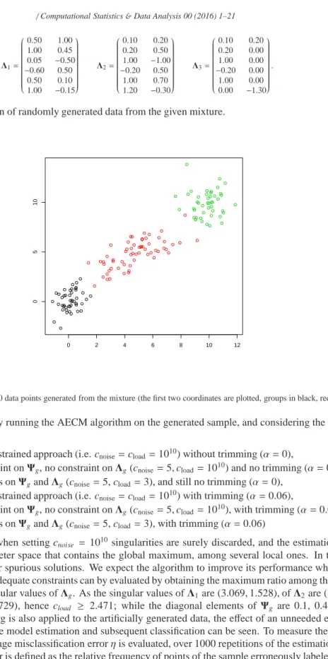
Λ1= 0.50 1.00 1.00 0.45 0.05 −0.50 −0.60 0.50
0.50 0.10 1.00 −0.15
Λ2=
0.10 0.20 0.20 0.50 1.00 −1.00 −0.20 0.50
1.00 0.70 1.20 −0.30
Λ3=
0.10 0.20 0.20 0.00 1.00 0.00 −0.20 0.00 1.00 0.00 0.00 −1.30
.
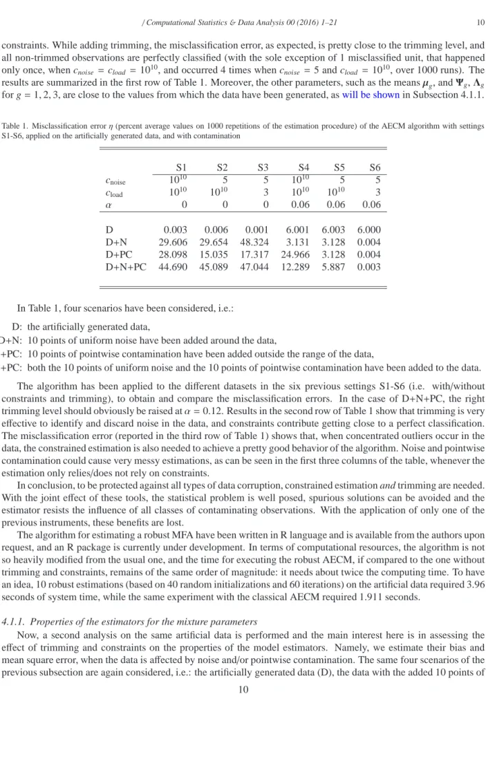
Figure 1 shows a specimen of randomly generated data from the given mixture.
0 2 4 6 8 10 12
0
5
10
Figure 1. A specimen of 150 data points generated from the mixture (the first two coordinates are plotted, groups in black, red and green) Our analysis begins by running the AECM algorithm on the generated sample, and considering the following six settings, namely:
S1. a ”virtually” unconstrained approach (i.e. cnoise=cload=1010) without trimming (α=0),
S2. an adequate constraint onΨg, no constraint onΛg(cnoise=5,cload=1010) and no trimming (α=0), S3. adequate constraints onΨgandΛg(cnoise=5, cload=3), and still no trimming (α=0),
S4. a ”virtually” unconstrained approach (i.e. cnoise=cload=1010) with trimming (α=0.06),
S5. an adequate constraint onΨg, no constraint onΛg(cnoise=5,cload=1010), with trimming (α=0.06), S6. adequate constraints onΨgandΛg(cnoise=5, cload=3), with trimming (α=0.06)
It is worth noticing that when setting cnoise =1010 singularities are surely discarded, and the estimation is allowed to move in a wide parameter space that contains the global maximum, among several local ones. In this situation, the estimation could incur spurious solutions. We expect the algorithm to improve its performance when giving the ”right” constraints. The adequate constraints can by evaluated by obtaining the maximum ratio among the eigenvalues ofΨgand among the singular values ofΛg. As the singular values ofΛ1are (3.069,1.528), ofΛ2are (3.777, 1.873) and of Λ3 are (2.091, 1.729), hence cload ≥ 2.471; while the diagonal elements of Ψg are 0.1, 0.4, and 0.2, so
constraints. While adding trimming, the misclassification error, as expected, is pretty close to the trimming level, and all non-trimmed observations are perfectly classified (with the sole exception of 1 misclassified unit, that happened only once, when cnoise =cload =1010, and occurred 4 times when cnoise=5 and cload =1010, over 1000 runs). The results are summarized in the first row of Table 1. Moreover, the other parameters, such as the meansµg, andΨg,Λg
for g=1,2,3, are close to the values from which the data have been generated, aswill be shownin Subsection 4.1.1.
Table 1. Misclassification errorη(percent average values on 1000 repetitions of the estimation procedure) of the AECM algorithm with settings S1-S6, applied on the artificially generated data, and with contamination
S1 S2 S3 S4 S5 S6
cnoise 1010 5 5 1010 5 5
cload 1010 1010 3 1010 1010 3
α 0 0 0 0.06 0.06 0.06
D 0.003 0.006 0.001 6.001 6.003 6.000 D+N 29.606 29.654 48.324 3.131 3.128 0.004 D+PC 28.098 15.035 17.317 24.966 3.128 0.004 D+N+PC 44.690 45.089 47.044 12.289 5.887 0.003
In Table 1, four scenarios have been considered, i.e.:
D: the artificially generated data,
D+N: 10 points of uniform noise have been added around the data,
D+PC: 10 points of pointwise contamination have been added outside the range of the data,
D+N+PC: both the 10 points of uniform noise and the 10 points of pointwise contamination have been added to the data.
The algorithm has been applied to the different datasets in the six previous settings S1-S6 (i.e. with/without constraints and trimming), to obtain and compare the misclassification errors. In the case of D+N+PC, the right trimming level should obviously be raised atα=0.12. Results in the second row of Table 1 show that trimming is very effective to identify and discard noise in the data, and constraints contribute getting close to a perfect classification. The misclassification error (reported in the third row of Table 1) shows that, when concentrated outliers occur in the data, the constrained estimation is also needed to achieve a pretty good behavior of the algorithm. Noise and pointwise contamination could cause very messy estimations, as can be seen in the first three columns of the table, whenever the estimation only relies/does not rely on constraints.
In conclusion, to be protected against all types of data corruption, constrained estimation and trimming are needed. With the joint effect of these tools, the statistical problem is well posed, spurious solutions can be avoided and the estimator resists the influence of all classes of contaminating observations. With the application of only one of the previous instruments, these benefits are lost.
The algorithm for estimating a robust MFA have been written in R language and is available from the authors upon request, and an R package is currently under development. In terms of computational resources, the algorithm is not so heavily modified from the usual one, and the time for executing the robust AECM, if compared to the one without trimming and constraints, remains of the same order of magnitude: it needs about twice the computing time. To have an idea, 10 robust estimations (based on 40 random initializations and 60 iterations) on the artificial data required 3.96 seconds of system time, while the same experiment with the classical AECM required 1.911 seconds.
4.1.1. Properties of the estimators for the mixture parameters
uniform noise (D+N), the data with the added 10 points of pointwise contamination (D+PC), and finally the data with both uniform noise and the pointwise contamination (D+N+PC).
We apply the algorithm for estimating a trimmed MFA model in all the four scenarios, exploring the six settings on
cnoise, cloadandαthat have been shown in Table 1. The benchmark of all simulations is given by the results obtained on artificial data drawn from a given MFA without outliers. In each experiment, a sample of size n=150 has been drawn 1000 times from the mixture described at the beginning of this Section, and the model parameters for the trimmed MFA have been estimated using the algorithm presented in the previous Section 3.2, by setting cnoise=cload=1010 (a virtually unconstrained solution) or cnoise =5,cload =3 for a constrained one, andα =0 for no trimming, while
α=0.06 orα=0.12 when adopting adequate trimming.
Notice that the considered estimators in each component are vectors (apart fromπg which are scalar quantities, for g=1, . . . ,G). We are interested in providing synthetic measures of their properties, such as bias and mean square
error (MSE). As usual, let ˆT be an estimator for the scalar parameter t, then the bias of ˆT is given by bias( ˆT )=E( ˆT )−t,
i.e. it is the signed absolute deviation of the expected valueE( ˆT ) from t. Therefore, we would have 6 biases for each
component of the meanµg, 6 for diag(Ψg) and 12 forΛg. On the other hand, MSE is defined as a scalar quantity, namelyE(|Tˆ −t|2) = trace(Var( ˆT ))+bias( ˆT )2, also for vector estimators. Hence, a synthesis of each parameter’s biases is adopted by considering the mean of their absolute values on each component. Below the bias, in Tables 2 and 3, the MSE is provided in parenthesis.
The results on bias and mean square error for the case of estimating the trimmed MFA with trimming but without constraints or viceversa, show the harmful effects of distorted inference. The only exception comes from D+N, where trimming is pretty able to cope with the contamination. On the other hand, when reasonable constraints cnoise =5,
/
C
o
m
p
u
ta
tio
n
a
l
S
ta
tis
tic
s
&
D
a
ta
A
n
a
ly
si
s
0
0
(2
0
1
6
)
1
–
2
1
1
data “D”, and for the artificial data plus noise “D+N”; labels from S1 to S6 denote the estimation settings
D D+N
S1 S2 S3 S4 S5 S6 S1 S2 S3 S4 S5 S6
π1 0 0 0 0.0154 0.0166 0.0167 -0.037 -0.1636 -0.2206 1e-04 0 0
(0) (0) (0) (2e-04) (3e-04) (3e-04) (0.0017) (0.0283) (0.0502) (0) (0) (0)
π2 0 0 0 -0.0227 -0.0229 -0.0238 -0.2835 0.065 0.4077 -1e-04 0 0
(0) (0) (0) (5e-04) (5e-04) (6e-04) (0.0807) (0.0058) (0.1677) (0) (0) (0)
π3 0 0 0 0.0073 0.0064 0.0071 0.3205 0.0985 -0.1871 0 0 0
(0) (0) (0) (1e-04) (0) (1e-04) (0.1031) (0.0113) (0.0365) (0) (0) (0)
µ1 0.001 0.001 0.003 0.003 0.004 0.006 0.215 2.289 5.468 0.002 0.003 0.002 (0.113) (0.117) (0.112) (0.124) (0.114) (0.12) (9.211) (99.165) (122.462) (0.118) (0.116) (0.11)
µ2 0.003 0.003 0.002 0.005 0.002 0.003 4.89 2.191 0.694 0.002 0.004 0.006
(0.132) (0.133) (0.131) (0.173) (0.179) (0.185) (74.119) (69.868) (34.888) (0.143) (0.126) (0.139)
µ3 0.006 0.003 0.001 0.003 0.004 0.003 1.492 1.026 10.338 0.004 0.004 0.002
(0.112) (0.11) (0.111) (0.122) (0.125) (0.123) (87.415) (91.361) (471.833) (0.109) (0.108) (0.115)
Ψ1 0.007 0.002 0.002 0.009 0.005 0.005 0.311 1.132 0.795 0.007 0.003 0.002
(0.009) (0.003) (0.003) (0.009) (0.004) (0.004) (58.795) (11.2) (6.278) (0.008) (0.003) (0.003)
Ψ2 0.029 0.045 0.045 0.074 0.1 0.1 9.194 0.445 0.355 0.033 0.047 0.047
(0.142) (0.05) (0.053) (0.169) (0.104) (0.106) (1837.338) (2.547) (2.248) (0.136) (0.053) (0.055)
Ψ3 0.168 0.04 0.04 0.174 0.048 0.047 0.422 0.316 0.928 0.166 0.041 0.041 (1.018) (0.053) (0.055) (0.952) (0.048) (0.048) (2.613) (1.375) (7.718) (0.989) (0.055) (0.054)
Λ1 0.526 0.529 0.533 0.523 0.526 0.551 0.558 0.537 0.525 0.523 0.527 0.517 (9.031) (9.127) (9.158) (9.064) (9.07) (9.547) (37.297) (296.817) (52.772) (9.064) (9.11) (8.954)
Λ2 0.585 0.576 0.56 0.573 0.566 0.575 0.668 0.633 0.553 0.573 0.574 0.58 (11.495) (11.369) (11.011) (11.326) (10.335) (10.634) (585.002) (205.661) (49.041) (11.326) (11.319) (11.569)
Λ3 0.333 0.332 0.341 0.34 0.342 0.337 0.346 0.363 0.346 0.34 0.341 0.337
(6.786) (7.448) (7.444) (6.888) (7.284) (7.224) (26.408) (22.941) (119.003) (6.888) (7.408) (7.503)
1
/
C
o
m
p
u
ta
tio
n
a
l
S
ta
tis
tic
s
&
D
a
ta
A
n
a
ly
si
s
0
0
(2
0
1
6
)
1
–
2
1
1
Table 3. Bias and MSE (in parentheses) of ˆπi, and bias as the sum of absolute deviations, followed by MSE (in parentheses) of the parameter estimators ˆµi,Ψi,Λi, for i=1,2,3 for the artificial
data plus pointwise contamination “D+PC”, and for the artificial data plus noise and pointwise contamination “D+N+PC”; labels from S1 to S6 denote the estimation settings
D+PC D+N+PC
S1 S2 S3 S4 S5 S6 S1 S2 S3 S4 S5 S6
π1 -0.0304 -0.0276 -0.0374 -0.0664 0 0 -0.218 -0.2116 -0.2163 -0.0534 1e-04 0
(0.001) (0.001) (0.0018) (0.0051) (0) (0) (0.0482) (0.0449) (0.0468) (0.003) (0) (0)
π2 -0.3076 -0.0868 -0.1376 -0.1742 0 0 0.4025 0.4418 0.4822 0.0316 -1e-04 0
(0.0947) (0.0077) (0.0193) (0.031) (0) (0) (0.1627) (0.1953) (0.2325) (0.0011) (0) (0)
π3 0.338 0.1144 0.175 0.2406 0 0 -0.1845 -0.2302 -0.2659 0.0218 0 0
(0.1143) (0.0133) (0.031) (0.0586) (0) (0) (0.0347) (0.0531) (0.0707) (6e-04) (0) (0)
µ1 0.346 0.931 1.365 1.918 0.002 0.003 21.143 18.651 20.535 5.233 0.006 0.001
(16.538) (30.237) (47.55) (75.165) (0.116) (0.112) (1416.987) (985.875) (881.201) (735.9) (0.114) (0.117)
µ2 8.59 2.682 4.489 6.005 0.005 0.004 1.146 0.534 0.001 2.208 0.007 0.003
(150.803) (102.543) (152.814) (147.795) (0.129) (0.135) (110.599) (49.885) (0.044) (344.79) (0.13) (0.132)
µ3 0.912 0.818 0.61 0.854 0.003 0.002 6.59 9.178 11.134 0.422 0.002 0.004 (3.31) (7.14) (5.662) (5.55) (0.111) (0.113) (383.624) (640.891) (381.857) (24.125) (0.11) (0.115)
Ψ1 0.012 0.052 0.07 0.032 0.003 0.003 0.069 0.509 0.636 0.028 0.003 0.002
(0.011) (0.072) (0.108) (0.027) (0.003) (0.003) (17.255) (3.089) (4.316) (0.021) (0.004) (0.003)
Ψ2 0.363 0.098 0.132 0.302 0.045 0.046 0.9 0.239 0.246 0.054 0.046 0.044 (0.969) (0.22) (0.285) (0.747) (0.052) (0.052) (101.563) (0.942) (0.788) (0.306) (0.051) (0.05)
Ψ3 0.692 0.12 0.186 0.241 0.041 0.04 8.865 1.006 1.176 0.124 0.042 0.042
(3.528) (0.332) (0.499) (0.747) (0.054) (0.054) (2101.106) (8.218) (10.605) (0.772) (0.053) (0.054)
Λ1 0.539 0.549 0.544 0.566 0.529 0.511 0.433 0.5 0.613 0.47 0.53 0.526
(9.581) (26.694) (18.72) (57.769) (9.111) (8.76) (470.528) (594.275) (257.523) (555.065) (9.126) (9.072)
Λ2 0.559 0.562 0.565 0.596 0.57 0.572 0.568 0.598 0.596 0.599 0.594 0.57
(10.083) (42.216) (27.648) (102.541) (11.248) (11.36) (151.272) (96.445) (38.347) (182.497) (11.736) (11.175)
Λ3 0.334 0.369 0.344 0.348 0.331 0.342 0.335 0.363 0.356 0.342 0.337 0.349 (11.31) (34.879) (15.699) (18.004) (7.337) (7.488) (470.156) (376.344) (193.749) (28.224) (7.468) (7.587)
1
The distributions of the estimators for the model parameters can be represented by box plots, and some of them are shown in Figure 2, namely with reference to ˆπ1 (upper panel), ˆµ1[1,1] (second panel), ˆΨ1[1,1] (third panel) and ˆΛ1[1,1] (bottom panel). In a direct comparison, the small efficiency reduction of the estimator when applying trimming and constraints on the true data (cases D/ S2-S6) can be seen, the effect of using only trimming when uniform noise has been added to data (case D+N/S4) is apparent; finally, the joint usage of trimming and constraints onΨgis shown to be effective to protect against all types of contamination.
4.2. Real data: the AIS data set
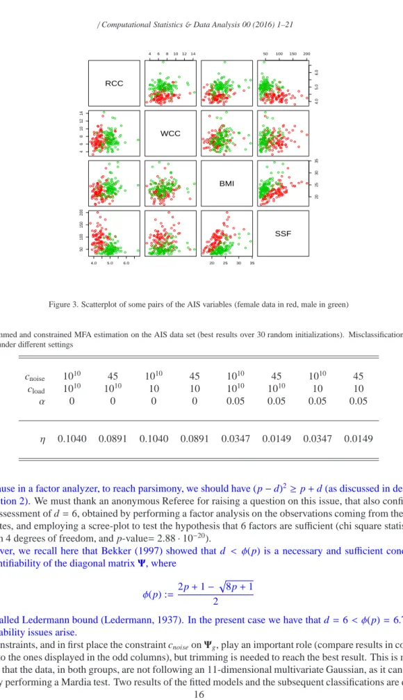
As an illustration, we apply the proposed technique to the Australian Institute of Sports (AIS) data, which is a famous benchmark dataset in the multivariate literature, originally reported by Cook and Weisberg (1994) and sub-sequently analyzed by Azzalini and Dalla Valle (1996), among many other authors. The dataset consists of p=11 physical and hematological measurements on 202 athletes (100 females and 102 males) in different sports, and is avail-able within the R package sn (Azzalini, A., 2011). The observed variavail-ables are: red cell count (RCC), white cell count (WCC), Hematocrit (Hc), Hemoglobin (Hg), plasma ferritin concentration (Fe), body mass index, weight/height2 (BMI), sum of skin folds (SSF), body fat percentage (Bfat), lean body mass (LBM), height, cm (Ht), weight, kg (Wt), apart from gender and kind of Sport. A partial scatterplot of the AIS dataset is given in Figure 3.
Our purpose is to provide a model for the entire dataset, and since the group labels (athlete’s gender) are provided in advance, the aim is to classify athletes by this feature.
Let us begin our analysis by fitting a mixture of multivariate Gaussian distributions, using the Mclust package in R. The routine mclustBIC, after fitting a set of normal mixture models, considering from 1 to 9 components in the mixture and different patterns for the covariance matrices, selects the best EEV model (ellipsoidal scatters, with equal volume and shape, different orientation of the component scatters) with G=2 components, providing the highest BIC value, i.e. BIC=−10251.6. Now, using this model to classify AIS data, 18 misclassified units are obtained, i.e., a misclassification error equal to 18/202=9.4%. The classification results are shown in Figure 4 (left panel).
To improve the classification, we may exploit the conjecture that a strong correlation exists between the hemato-logical and physical measurements. Therefore, a mixture of factor analyzers may be estimated, assuming the existence of some underlying unknown factors (like nutritional status, hematological composition, overweight status indices, and so on) which jointly explain the observed measurements. Through the factors, the aim is to find a perspective on data which disentangles the overlapping components. To avoid variables having a greater impact in the model (which is not affine equivariant) due to different scales, before performing the estimation, the variables have been divided by their interquartile range. We begin by adopting the pGmm package from R, that fits mixtures of factor analyzers with patterned covariances. Parsimonious Gaussian mixtures are obtained by constraining the loadingsΛgand the errors
Ψgto be equal or not among the components. We employed the routine pGmmEM, considering from 1 to 9 compo-nents, and number of underlying factors d ranging from 1 to 6, with 30 different random initializations, to provide the best iteration (in terms of BIC) for each case. The best model is a CUU mixture model with d=4 factors and G=3 components, with BIC=−3127.424. CUU means “Constrained” loading matricesΛg= Λand “Unconstrained” error matricesΨg =ωg∆g, where∆gare normalized diagonal matrices andωg is a real value varying across components. Using this model to classify athletes, we got 109 misclassified units and we discarded it.
As a second attempt using pGmm, a UUU model has been estimated by setting G =2 components, and d =6. The acronym UUU means that the estimation of loadingsΛgand errorsΨg is unconstrained. Based on 30 random starts, the best UUU model has BIC=−3330.306, and the consequent classification of the AIS dataset produces 72 misclassified units (misclassification error=35.6%, see the right panel in Figure 4).
Finally, we want to show the performance of our trimmed and constrained estimation for MFA on the AIS data. All the results are generated by the procedure described in Section 3.2, based on 30 random initializations and returning the best obtained solution of the parameters, in terms of the highest value of the final likelihood. We see that the best solution, with only 3 misclassified points, has been obtained by combining trimming (α=0.05) and the constrained estimation ofΨg(cnoise=45) andΛg(cload=10), with d=6.
Notice that the choice of G=2 and d=6 could be motivated by estimating all models within a range of values for
G and d, and choosing the pair of values providing the best BIC. A trimmed version of the BIC=2Ltrim(x; ˆθ)−k log n∗
/ C o m p u ta tio n a l S ta tis tic s & D a ta A n a ly si s 0 0 (2 0 1 6 ) 1 – 2 1 1
0.0 0.2 0.4 0.6 0.8 1.0
−80 −60 −40 −20
0
0 1 2 3 4
D / S1 D / S2 D / S3 D / S4 D / S5 D / S6
D+N / S1 D+N / S2 D+N / S3 D+N / S4 D+N / S5 D+N / S6
D+PC / S1 D+PC / S2 D+PC / S3 D+PC / S4 D+PC / S5 D+PC / S6
D+N+PC / S1 D+N+PC / S2 D+N+PC / S3 D+N+PC / S4 D+N+PC / S5 D+N+PC / S6
−30 −20 −10
0
10 20 30
RCC
4 6 8 1012 14 50 100 150 200
4.0
5.0
6.0
4
6
8
10
12
14
WCC
BMI
20
25
30
35
4.0 5.0 6.0
50
100
150
200
20 25 30 35
SSF
Figure 3. Scatterplot of some pairs of the AIS variables (female data in red, male in green)
Table 4. Trimmed and constrained MFA estimation on the AIS data set (best results over 30 random initializations). Misclassification errorη(in percentage) under different settings
cnoise 1010 45 1010 45 1010 45 1010 45
cload 1010 1010 10 10 1010 1010 10 10
α 0 0 0 0 0.05 0.05 0.05 0.05
η 0.1040 0.0891 0.1040 0.0891 0.0347 0.0149 0.0347 0.0149
d=6 because in a factor analyzer, to reach parsimony, we should have (p−d)2≥p+d (as discussed in detail at the
end of Section 2).We must thank an anonymous Referee for raising a question on this issue, that also confirmed our
previous assessment of d=6, obtained by performing a factor analysis on the observations coming from the group of male athletes, and employing a scree-plot to test the hypothesis that 6 factors are sufficient (chi square statistic equal to 97.81 on 4 degrees of freedom, and p-value=2.88·10−20).
Moreover, we recall here that Bekker (1997) showed that d < φ(p) is a necessary and sufficient condition for
global identifiability of the diagonal matrixΨ, where
φ(p) :=2p+1−
p
8p+1
2
is the so-called Ledermann bound (Ledermann, 1937). In the present case we have that d=6 < φ(p)=6.78, hence
no identifiability issues arise.
RCC
4 6 810 12 14 50 100 150 200
4.0
5.0
6.0
4
6
8
10
12
14
WCC
BMI
20
25
30
35
4.0 5.0 6.0
50
100
150
200
20 25 30 35 SSF
RCC
4 6 810 12 14 50 100 150 200
4.0
5.0
6.0
4
6
8
10
12
14
WCC
BMI
20
25
30
35
4.0 5.0 6.0
50
100
150
200
20 25 30 35 SSF
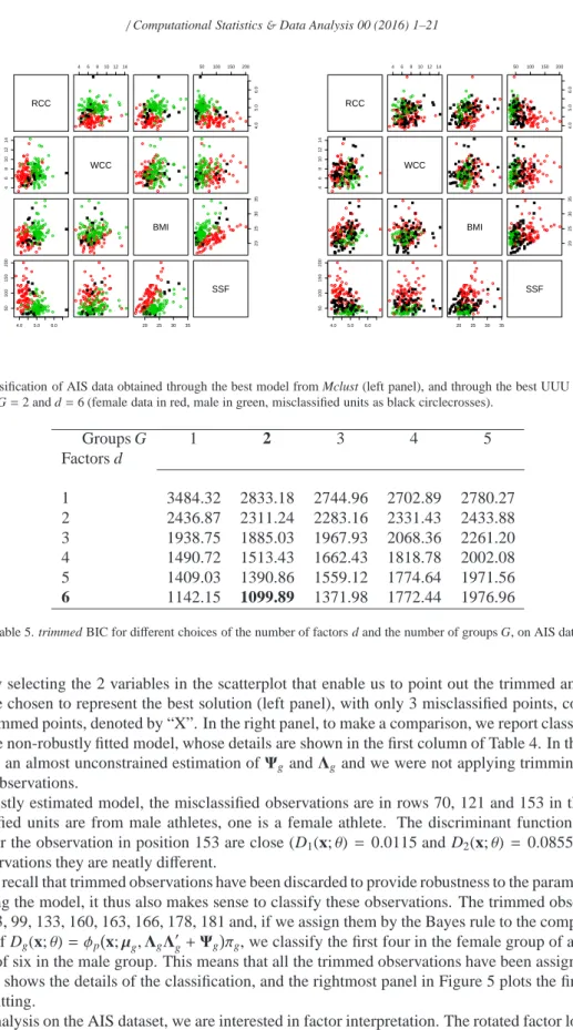
Figure 4. The classification of AIS data obtained through the best model from Mclust (left panel), and through the best UUU model from pGmm (right panel) with G=2 and d=6 (female data in red, male in green, misclassified units as black circlecrosses).
Groups G 1 2 3 4 5
Factors d
1 3484.32 2833.18 2744.96 2702.89 2780.27 2 2436.87 2311.24 2283.16 2331.43 2433.88 3 1938.75 1885.03 1967.93 2068.36 2261.20 4 1490.72 1513.43 1662.43 1818.78 2002.08 5 1409.03 1390.86 1559.12 1774.64 1971.56 6 1142.15 1099.89 1371.98 1772.44 1976.96
Table 5. trimmed BIC for different choices of the number of factors d and the number of groups G, on AIS data.
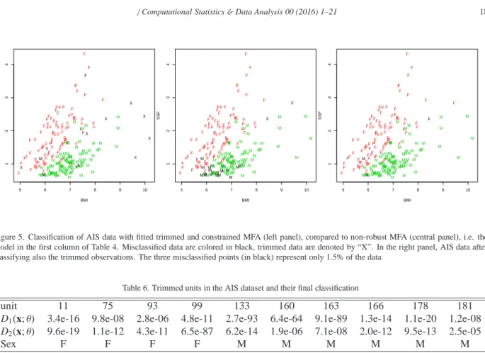
in Figure 5, by selecting the 2 variables in the scatterplot that enable us to point out the trimmed and misclassified units. We have chosen to represent the best solution (left panel), with only 3 misclassified points, colored in black, and with 10 trimmed points, denoted by “X”. In the right panel, to make a comparison, we report classification results obtained by the non-robustly fitted model, whose details are shown in the first column of Table 4. In this second case, we were doing an almost unconstrained estimation ofΨgandΛg and we were not applying trimming, obtaining 21 misclassified observations.
In the robustly estimated model, the misclassified observations are in rows 70, 121 and 153 in the AIS dataset. Two misclassified units are from male athletes, one is a female athlete. The discriminant function of the mixture components for the observation in position 153 are close (D1(x;θ)= 0.0115 and D2(x;θ) =0.0855), while for the other two observations they are neatly different.
Finally, we recall that trimmed observations have been discarded to provide robustness to the parameter estimation. After estimating the model, it thus also makes sense to classify these observations. The trimmed observations are in rows 11, 75, 93, 99, 133, 160, 163, 166, 178, 181 and, if we assign them by the Bayes rule to the component g having greater value of Dg(x;θ)=φp x;µg,ΛgΛ′g+Ψgπg, we classify the first four in the female group of athletes, and the second group of six in the male group. This means that all the trimmed observations have been assigned to their true group. Table 6 shows the details of the classification, and the rightmost panel in Figure 5 plots the final result of the robust model fitting.
F F F F F F F F F F X F F F F F F F F F F F F F F F F F F F F F F F F F F F F F F F F F F F F F F F F F F F F F F F F F F F F F F F F F F F F F F F X F FF F F F F F F F F
F FF
F F F X F F FF F X F M M M M M M M M M M M M M M M M M M M M M M M M M M M M M M M M X M M M M M M M M MM M M M M M M MM MM M
M M M M
M X M M X M MX M M M M M M M M M M M X M M X M M M M M M M M M M M M M M M M M M M M M
5 6 7 8 9 10
1 2 3 4 BMI SSF F F F F F F F F F F F F F F F F F F F F F F F F F F F F F F F F F F F F F F F F F F F F F F F F F F F F F F F F F F F F F F F F F F F F F F F F F F F F F F F F F F F F F F
F FF
F F F F F F FF F F F M M M M M M M M M M M M M M M M M M M M M M M M M M M M M M M M M M M M M M M M M MM M M M M M M MM MM M
M M M M
M M M M M M MM M M M M M M M M M M M M M M M M M M M M M M M M M M M M M M M M M M M M
5 6 7 8 9 10
1 2 3 4 BMI SSF F F F F F F F F F F F F F F F F F F F F F F F F F F F F F F F F F F F F F F F F F F F F F F F F F F F F F F F F F F F F F F F F F F F F F F F F F F F F FF F F F F F F F F
F FF
F F F F F F FF F F F M M M M M M M M M M M M M M M M M M M M M M M M M M M M M M M M M M M M M M M M M MM M M M M M M MM MM M
M M M M
M M M M M M MM M M M M M M M M M M M M M M M M M M M M M M M M M M M M M M M M M M M M
5 6 7 8 9 10
1 2 3 4 BMI SSF
Figure 5. Classification of AIS data with fitted trimmed and constrained MFA (left panel), compared to non-robust MFA (central panel), i.e. the model in the first column of Table 4. Misclassified data are colored in black, trimmed data are denoted by “X”. In the right panel, AIS data after classifying also the trimmed observations. The three misclassified points (in black) represent only 1.5% of the data
Table 6. Trimmed units in the AIS dataset and their final classification
unit 11 75 93 99 133 160 163 166 178 181
D1(x;θ) 3.4e-16 9.8e-08 2.8e-06 4.8e-11 2.7e-93 6.4e-64 9.1e-89 1.3e-14 1.1e-20 1.2e-08
D2(x;θ) 9.6e-19 1.1e-12 4.3e-11 6.5e-87 6.2e-14 1.9e-06 7.1e-08 2.0e-12 9.5e-13 2.5e-05
Sex F F F F M M M M M M
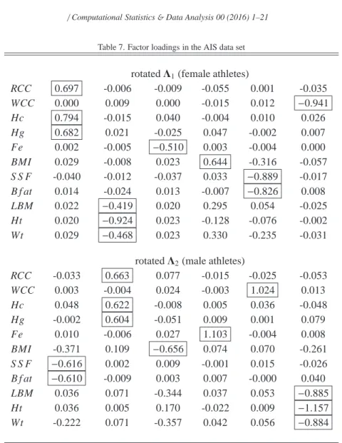
in Table 7. We observe that the two groups highlight the same factors, while in a slightly different order of importance. The first factor for the group of observations for female athletes, may be labelled as a hematological factor, with a very high loading on Hc, followed by RCC and Hg. The second factor, loading heavily on Ht, and in a lesser extent on Wt and LBM, may be denoted as a general nutritional status. The third and fourth factors are related only to Fe and BMI, respectively. The fifth factor can be viewed as an overweight assessment index, since S S F and B f at load highly on it. The sixth factor is related only to WCC. Noticing that WCC is not joined to the hematological factor, we observe that the specific role of lymphocytes, cells of the immune system that are involved in defending the body against both infectious disease and foreign invaders, seems to be pointed out. Analogous comments may be done on the factor loadings for the group of male athletes.
We would like to add a final remark on this data analysis. When approaching the AIS dataset, we run a Mardia test on both groups and measured asymmetry and kurtosis, finding that both are significantly different from the Gaussian case. Hence one may argue that a mixture of two skew distributions, as in Lin et al. (2014a), is more suited for this dataset. Unfortunately, the obtained misclassification error, comparing different skew components, ranges from 4.5% to 5.9%. We want to show here that trimming is a convenient and competitive tool to be adopted, when one tail (skewness) or both tails (kurtosis) are contaminated in the data. As a general principle, trimming enables robust estimation of the location and scatter, and may offer an effective alternative to the adoption of more parameterized skew models. Our results show that we estimated the core of the data through a Gaussian density, obtaining such a good classification. We therefore argue that the flexibility obtained by the robust approach may provide a pretty good fit, even in the presence of some asymmetry in data tails.
5. Concluding remarks
We propose a robust estimation for the mixture of Gaussian factor model by adopting trimming and constrained
Table 7. Factor loadings in the AIS data set rotatedΛ1(female athletes)
RCC 0.697 -0.006 -0.009 -0.055 0.001 -0.035
WCC 0.000 0.009 0.000 -0.015 0.012 −0.941
Hc 0.794 -0.015 0.040 -0.004 0.010 0.026
Hg 0.682 0.021 -0.025 0.047 -0.002 0.007
Fe 0.002 -0.005 −0.510 0.003 -0.004 0.000
BMI 0.029 -0.008 0.023 0.644 -0.316 -0.057
S S F -0.040 -0.012 -0.037 0.033 −0.889 -0.017
B f at 0.014 -0.024 0.013 -0.007 −0.826 0.008
LBM 0.022 −0.419 0.020 0.295 0.054 -0.025
Ht 0.020 −0.924 0.023 -0.128 -0.076 -0.002
Wt 0.029 −0.468 0.023 0.330 -0.235 -0.031
rotatedΛ2(male athletes)
RCC -0.033 0.663 0.077 -0.015 -0.025 -0.053
WCC 0.003 -0.004 0.024 -0.003 1.024 0.013
Hc 0.048 0.622 -0.008 0.005 0.036 -0.048
Hg -0.002 0.604 -0.051 0.009 0.001 0.079
Fe 0.010 -0.006 0.027 1.103 -0.004 0.008
BMI -0.371 0.109 −0.656 0.074 0.070 -0.261
S S F −0.616 0.002 0.009 -0.001 0.015 -0.026
B f at −0.610 -0.009 0.003 0.007 -0.000 0.040
LBM 0.036 0.071 -0.344 0.037 0.053 −0.885
Ht 0.036 0.005 0.170 -0.022 0.009 −1.157
Wt -0.222 0.071 -0.357 0.042 0.056 −0.884
a trimming procedure in the iterations of the EM algorithm. The key idea is that a small portion of observations, which are highly unlikely to occur under the current fitted model assumption, are discarded from contributing to the parameter estimates. Furthermore, to reduce spurious solutions and avoid singularities of the likelihood, a constrained ML estimation for the component covariances has been implemented. Results from the Monte Carlo experiments show that the bias and MSE of the estimators, in several cases of contaminated data, are comparable to results obtained on data without noise. Finally, the analysis on a real dataset illustrates that robust estimation leads to better classification and provides direct interpretation of the factor loadings.
Moreover, larger values of the constraints could lead to higher values of G, since new components with few, almost collinear observations may arise. With respect to the choice of the specific values for the constraints, our experience tells us that a moderate interval of values for cloadand cnoiseproduces almost the same estimation and exactly the same classification. Also, from an interpretative point of view, this corresponds to the fact that, generally, the user has some intuition (or rough knowledge) about the order of magnitude of these constraints, and this partial information can be incorporated into the estimation. The encouraging results obtained here suggest that a deeper discussion of these implementation details could be developed as a future work.
As a final remark, following the suggestions for further investigation we received from an unknown referee, the proposed method can also be extended to accommodate missing values, as in Wang (2015); and much faster convergence to the EM-based algorithm could be improved along the lines of Zhao and Yu (2008).
Acknowledgements
The authors would like to thank two anonymous referees for many interesting and helpful comments that led to a clearer presentation of the material. This research is partially supported by the Spanish Ministerio de Ciencia e Innovaci´on, grant MTM2014-56235-C2-1-P, by Consejer´ıa de Educaci´on de la Junta de Castilla y Le´on, grant VA212U13, by grant FAR 2015 from the University of Milano-Bicocca and by a grant FIR 2014 from the University of Catania.
References
Azzalini A., R package sn: The skew-normal and skew-t distributions (version 0.4-17), URL http://azzalini. stat. unipd. it/SN, (2011).
Azzalini A., Dalla Valle A., The multivariate skew-normal distribution, Biometrika, 83 (4), 715–726, (1996).
Baek J., McLachlan G., Flack L., Mixtures of Factor Analyzers with Common Factor Loadings: Applications to the Clustering and Visualization of High-Dimensional Data, IEEE Transactions on Pattern Analysis and Machine Intelligence, 32 (7), 1298 –1309, (2010).
Baek J., McLachlan G., Mixtures of common t-factor analyzers for clustering high-dimensional microarray data, Bioinformatics, 27 (9), 1269– 1276, (2011).
Bernaards C. A., Jennrich R. I. , Gradient projection algorithms and software for arbitrary rotation criteria in factor analysis, Educational and
Psychological Measurement, 65 (5), 676–696, (2005).
Bekker P. A., ten Berge J. M. F. , Generic global identification in factor analysis, Linear Algebra and its Applications, 264, 255–263, (1997). Bickel D.R., Robust cluster analysis of microarray gene expression data with the number of clusters determined biologically, Bioinformatics, 19 (7),
818–824, (2003).
Bishop C. M., Tipping M. E., A Hierarchical Latent Variable Model for Data Visualization, IEEE Transactions on Pattern analysis and Machine
Intelligence , 20, 281–293, (1998).
Browne M. W., An overview of analytic rotation in exploratory factor analysis, Multivariate Behavioral Research, 36 (1), 111–150, (2001). Campbell J., Fraley C., Murtagh F., Raftery A., Linear flaw detection in woven textiles using model-based clustering, Pattern Recognition Letters,
18 (14), 1539 – 1548, (1997).
Cook R. D., Weisberg S., An introduction to regression graphics, vol. 405, John Wiley & Sons, 1994.
Coretto P., Hennig C., Maximum likelihood estimation of heterogeneous mixtures of Gaussian and uniform distributions, Journal of Statistical
Planning and Inference, 141 (1) 462–473, (2011) .
Fokou´e E., Titterington D., Mixtures of factor analysers. Bayesian estimation and inference by stochastic simulation, Machine Learning, 50 (1-2), 73–94, (2003).
Fraley C., Raftery A. E., How Many Clusters? Which Clustering Method? Answers Via Model-Based Cluster Analysis, Computer Journal, 41 (8), 578–588, (1998).
Fritz H., Garc´ıa-Escudero L., Mayo-Iscar A., A fast algorithm for robust constrained clustering, Computational Statistics&Data Analysis, (61),
124–136, (2013).
Gallegos M., Ritter G., Trimmed ML estimation of contaminated mixtures, Sankhya (Ser. A), (71), 164–220, (2009).
Garc´ıa-Escudero L. A., Gordaliza A., Matr´an C., Mayo-Iscar A., A General Trimming Approach to Robust Cluster Analysis, The Annals of
Statistics, 36 (3) 1324–1345 (2008).
Garc´ıa-Escudero L. A., Gordaliza A., Matr´an C., Mayo-Iscar A., Exploring the Number of Groups in Robust Model-Based Clustering, Statistics
and Computing, 21 (4), 585–599, (2011).
Garc´ıa-Escudero L., Gordaliza A., Mayo-Iscar A., A constrained robust proposal for mixture modeling avoiding spurious solutions, Advances in
Data Analysis and Classification, 8 (1), 27–43, (2014).
Ghahramani Z., Hilton G., The EM algorithm for mixture of factor analyzers, Techical Report CRG-TR-96-1, (1997).
Greselin F., Ingrassia S., Maximum likelihood estimation in constrained parameter spaces for mixtures of factor analyzers, Statistics and
Comput-ing, 25, 215–226, (2015).
Hathaway R., A constrained formulation of maximum-likelihood estimation for normal mixture distributions, The Annals of Statistics, 13 (2), 795–800, (1985).
Ingrassia S., A likelihood-based constrained algorithm for multivariate normal mixture models, Statistical Methods&Applications, 13, 151–166,
(2004).
Ingrassia S., Rocci R., Constrained monotone EM algorithms for finite mixture of multivariate Gaussians, Computational Statistics&Data Analysis,
51, 5339–5351, (2007).
Ledermann, W., On the rank of the reduced correlational matrix in multiple-factor analysis, Psychometrika, 2 (2), 85-93, (1937).
Lin T.-I., Ho H. J., Lee C. R., Flexible mixture modelling using the multivariate skew-t-normal distribution, Statistics and Computing, 24 (4), 531-546, (2014).
Lin T.-I., McNicholas P. D., Ho H. J., Capturing patterns via parsimonious t mixture models, Statistics&Probability Letters, 88, 80–87, (2014).
Maitra R., Clustering Massive Datasets With Application in Software Metrics and Tomography, Technometrics, 43 (3), 336–346, (2001). Maitra R., Initializing partition-optimization algorithms, IEEE/ACM Transactions on Computational Biology and Bioinformatics 6 (1) 144–157,
(2009).
McLachlan G. J., Bean R. W., Maximum likelihood estimation of mixtures of t factor analyzers, Technical Report, University of Queensland, (2005).
McLachlan G., Peel D., Robust mixture modelling using the t distribution, Statistics and Computing, 10 (4) 335–344, (2000).
McLachlan G., Peel D., Mixtures of factor analyzers, in: Proceedings of the Seventeenth International Conference on Machine Learning, P. Langley (Ed.)., San Francisco: Morgan Kaufmann, 599–606, (2000a).
McLachlan G. J., Peel D., Finite Mixture Models, John Wiley & Sons, New York, (2000b).
McNicholas P., Murphy T., Parsimonious Gaussian mixture models, Statistics and Computing, 18 (3), 285–296, (2008).
Neykov N., Filzmoser P., Dimova R., Neytchev P., Robust Fitting of Mixtures Using the Trimmed Likelihood Estimator, Computational Statistics
&Data Analysis, 52 (1), 299–308, (2007).
R. D. C. Team, R: A Language and Environment for Statistical Computing, R Foundation for Statistical Computing, Vienna, Austria, URL
http://www.R-project.org, (2013).
Rousseeuw P. J., Van Driessen K., A Fast Algorithm for the Minimum Covariance Determinant Estimator, Technometrics, 41, 212–223, (1999). Steane M. A., McNicholas P. D., R. Y. Yada, Model-based classification via mixtures of multivariate t-factor analyzers, Communications in
Statistics-Simulation and Computation, 41 (4), 510–523, (2012).
Stewart C. V., Robust parameter estimation in computer vision, SIAM review, 41 (3), 513–537, (1999).
Tipping M. E., Bishop C. M., Mixtures of probabilistic principal component analyzers, Neural computation, 11 (2), 443–482, (1999).
Wang, W. L., Mixtures of common t-factor analyzers for modeling high-dimensional data with missing values, Computational Statistics&Data Analysis, 83, 223–235, (2015).