i
UNIVERSIDAD DE VALLADOLID
ESCUELA DE INGENIERIAS INDUSTRIALES
Grado en Ingeniería Mecánica
Simulación del efecto de la temperatura en un
aparato de Respuesta por Frecuencia
Autor:
Tomillo Álvarez, Ignacio
Rey Martínez, Francisco Javier
ii
Valladolid, mes y año.
TFG REALIZADO EN PROGRAMA DE INTERCAMBIOTÍTULO: Simulation of temperature effect in a Frequency Response apparatus
ALUMNO: Ignacio Tomillo Álvarez
FECHA: 25 Febrero 2016
CENTRO: Facultad de Ingeniería Mecánica
iii
Abstract
El objetivo principal de este proyecto es determinar el efecto que la temperatura tendrá en un aparato de Respuesta por Frecuencia. En dicho aparato se encuentra un material poroso que actúa como catalizador, del cual se pretenden obtener las constantes de difusión y adsorción para optimizar sus propiedades.
El funcionamiento de este sistema consiste en comprimir y expandir un gas (nitrógeno en este caso) de forma que el catalizador entre en funcionamiento. El cambio de presión, así como las fuerzas viscosas podrían hacer que la temperatura del sistema aumente afectando el funcionamiento del catalizador.
Para esto se utiliza el programa COMSOL Multiphysics, el cual permite modelar y poner en marcha el aparato comprobando, por medio de diferentes campos científicos (transferencia de calor, flujo laminar y movimiento del mallado), el cambio de temperatura que sufre el sistema. Teniendo en cuenta las especificaciones del material poroso se llega a la conclusión de que dicha variación no afecta al funcionamiento de éste.
Keywords
iv
Kek
Simulation of temperature effect in a
Frequency Response apparatus
Ignacio Tomillo Álvarez
Betreuender Hochschullehrer: Prof. Dr. Cornelia Breitkopf
Bearbeitungszeitraum: 10.2015 – 02.2016
Fakultät Maschinenwesen. Institut für Energietechnik, Professur für Thermodynamik
i
Table of contents
1 Introduction ... 1
2 Objectives ... 2
3 Theoretical contents ... 3
3.1 Isentropic compression ... 4
3.2 Heat generation and conservation of energy... 6
3.2.1 Heat generation due to pressure changes within the fluid ... 6
3.2.2 Heat generation due to the fluid viscosity ... 7
3.3 Frequency Response and diffusion and adsorption processes ... 7
4 Experimental setup... 10
5 Computational setup ... 13
5.1 Represented components in COMSOL Multiphysics ... 13
5.2 Simulation of the FR system ... 14
6 Simulations and interface settings ... 18
6.1 Geometry ... 18
6.2 Materials ... 21
6.3 Description of the interfaces ... 22
6.3.1 Moving mesh ... 23
6.3.2 Laminar flow 1 ... 26
6.3.3 Laminar flow 2 ... 30
6.3.4 Heat Transfer ... 31
6.4 Mesh ... 33
6.5 Study ... 39
7 Results and problems faced ... 43
7.1 Obtained results and commentaries ... 43
7.1.1 Checking of pressure and temperature values in the model ... 44
7.1.2 Pressure variation in different points of the setup ... 46
7.1.3 Temperature comparison between volume-modulation unit and reactor... 48
7.1.4 Maximum temperature of the system ... 49
7.2 Problems faced ... 50
8. Final conclusions ... 53
ii
iii
Table of figures
Figure 1: Pressure variation in presence of a porous material ... 8
Figure 2: Complete experimental setup ... 10
Figure 3: Setup components that will be analysed in the model ... 11
Figure 4: Main parameters of the function that describes the movement ... 15
Figure 5: Displacement function of the bellows, wave (x) ... 16
Figure 6: Velocity function of the bellows, velocity(x) ... 16
Figure 7: Cross section of the setup required for this model ... 18
Figure 8: First geometry of the model ... 19
Figure 9: Complete geometry of the model including the air domains ... 20
Figure 10: Diagram of the materials used for the model ... 22
Figure 11: “Add physics” menu ... 23
Figure 12: Boundary displacement that generates the movement ... 24
Figure 13: Axis is set to zero horizontal movement ... 25
Figure 14: Outer and lower parts of the moving mesh remain still ... 25
Figure 15: Example of the linear extrusion function ... 28
Figure 16: Selection of velocity for the wall node ... 29
Figure 17: Open boundary characteristics and selected boundaries ... 30
Figure 18: Geometry before and after the domain division ... 33
Figure 19: Mesh calibration according to the physics ... 34
Figure 20: Predefined mesh sizes from the finest to the largest ... 34
Figure 21: Values of size parameters for Mesh 1 ... 35
Figure 22: Boundary layer parameters ... 36
Figure 23: Boundary layers in both sides of the bellow boundaries ... 37
Figure 24: Velocity results for the comparison of the different types of mesh ... 38
Figure 25: Initial and maximum step new values ... 41
Figure 26: Features of Segregated Step used for “Laminar Flow” variables ... 42
Figure 27: Average absolute pressure in the system ... 44
Figure 28: Average temperature in the system ... 45
Figure 29: Comparison between different pressure functions ... 46
Figure 30: Average temperature at the volume-modulation unit and at the reactor ... 48
Figure 31: Maximum temperatures reached in the system ... 49
Figure 32: Temperature variation distribution at points 1 and 2, respectively, from Fig. 31 ... 50
Figure 33: Pressure variation during the compression process ... 51
iv
List of tables
Table 1: List of parameters inserted in Comsol Multiphysics ... 13
Table 2: Density variables used in the model ... 26
Table 3: Simulation time for every mesh type ... 39
Table 4: Volume variation of the nitrogen during the compression ... 43
Table 5: Pressure values for the upper domain ... 47
Table 6: Pressure values for the pipe domain ... 47
1
1 Introduction
The environmental pollution affects our health directly and it is more notable every day, as our population keeps growing. There are natural ways of contamination such as volcanic eruptions or decomposition of living beings, but it is the human polluting factors which really concern us. Some artificial polluting processes are automobile emissions, chemical odours and factory smokes and some examples of gases that are expelled to the atmosphere are carbon monoxide (CO), carbon dioxide (CO2), hydrocarbon, oxides of sulphur (SOx) and oxides of nitrogen (NOx) [1].
In some cases, like vehicle emissions, one way of avoiding these emissions is by using catalysts. A catalyst is a substance that increases the rate of reaction without being consumed or changed [2]. Catalysts can be divided in homogeneous - they have the same phase as reactants and products - and heterogeneous – they are present in different phase, usually solid, which helps with the catalyst separation from the product and makes the reaction more tolerant to extreme operating conditions. One type of heterogeneous catalyst is a zeolite. A zeolite is a porous solid with pores of molecular dimensions size – 0.3-2.0 nm – which are delineated by their crystal structure [3].
Zeolites must be characterized to optimize their performance. The experiment that inspires this work has been built in order to make a microkinetic analysis, in which catalytic reactions are studied to learn about diffusion and adsorption conditions [4]. There are several methods which permit us to achieve this. In this case, a Frequency Response (FR) apparatus is used. It changes the volume of the system by compressing and expanding the gas that is inside, favouring both diffusion and sorption processes [5], as the porous material lies at the bottom of the reactor.
When gases are compressed their temperature rise. Convection will appear because of the velocity that is added to the fluid and conduction too. Temperature changes must be measured and it must be decided, whether they are important or not, so that they can be taken into account for future experiments.
In order to measure this temperature exchange in the real experiment, very specific methods would be needed, as it is a difficult process. Therefore, computer simulations are preferable for approaching our objectives. The conditions of the lab and the experiment itself can be described quite exactly, as well as the geometry and materials of every part that is being used. Additionally, some parts can be optimized and it is possible to change the fluids or the geometry and repeat the experiment. The modelling tool used here is COMSOL Multiphysics 4.4.
2
2 Objectives
The main aim of the experimental investigation is to obtain the adsorption and diffusion coefficients of the gas interacting with the catalyst in the reactor, as it was mentioned before. In order to achieve this, several elements and conditions which affect it directly must be checked. One of them is the temperature exchange with its surroundings.
Up to now the experiment was considered to be adiabatic. When working under ideal conditions, there is no heat exchange between the gas and its surroundings, so the variation of heat in the system is zero [7].
From now on, the conditions are no longer adiabatic. When the fluid is compressed the total volume decreases and the pressure increases. This makes the temperature of the inner fluid (N2) rise. As the system is not adiabatic, convection and conduction will appear, and there will be a heat exchange between the system and its surroundings.
The creation of a new model is necessary in order to analyse the heat exchange – new variable – correctly. The temperature may affect the final result by heating the solid elements that are part of the experiment or affecting the characteristics of the porous material.
3
3 Theoretical contents
The part of the experiment that concerns us consists of a closed system where a gas (nitrogen in this case) is compressed and expanded periodically. The first assumption to be made is that N2 has ideal gas properties. This means that the ideal gas equation will be used,
(Eq.1)
where p is the gas pressure in Pa, V is the volume in m3, R is the gas constant in J/Kg·K, m is the mass in kg and T is temperature in K.
By applying the First Law of Thermodynamics,
̇ ̇ ∑ ̇ ∑ ̇ (Eq.2)
where dE/dt is the energy variation, W is the power due to external work, Q is the heat power within the system and the last two terms are the inlet and outlet of power due to enthalpy, fluid velocity and gravity, respectively. But as the system is closed, there is no inlet or outlet. The latter equation (Eq.2) then is:
̇ ̇ (Eq.3)
The Second Law of Thermodynamics states that [4],
̇ ̇ ∑ ̇ ∑ ̇
(Eq.4)
4
̇ ̇
(Eq.5)
3.1 Isentropic compression
In order to obtain some characteristic values and results previous to doing the simulation, a series of assumptions can be made so that the previous equations can be simplified.
Assuming that the system is adiabatic once the nitrogen is introduced, the last term in (Eq.3) cancels out. The resulting equation is:
̇
(Eq.6)
This means that the variation of internal energy depends just on the external work that affects the system, in this case, the movement of the bellows.
If the process is reversible the last two terms of (Eq.5) are equal to zero. The resulting equation is:
(Eq.7)
There is no entropy variation in this process so the experiment will work on isentropic conditions. Therefore we know that the internal energy variation and the external work expressions are, respectively [8]:
∫ (Eq.8)
∫ (Eq.9)
5 ∫ ∫
∫ ∫
(Eq.10)
( ) ( ) (Eq.11)
In order to group the exponents, the heat capacity ratio, k, and the relation between R and cv will be used according to our adiabatic system and ideal gas conditions, respectively [7]:
(Eq.12)
(Eq.13)
Consequently, equation (Eq.9) changes to:
( )
(Eq.14)
To obtain the relation between temperatures and pressures, the volume-temperature relation (Eq.12) along with the ideal gas equation (Eq.1) can be related:
( )
(Eq.15)
6
3.2 Heat generation and conservation of energy
In this experiment there are no external heat sources that affect the fluid from the start of the process and no temperature difference between the inside of the experiment and the surroundings. This means that the heat in its entirety is generated by the fluid interaction movement.
The equation which represents this heat exchange is the conservation of energy:
[
⃗⃗⃗⃗ ]
(Eq.16)
By using the ideal gas equation (Eq.1) and the relation between enthalpy and temperature – which can also be used because nitrogen is considered an ideal gas – the latter equation can be simplified so that the temperature will be the only unknown variable [9].
(Eq.17)
[
]
(Eq.18)
The term Qi represents the external heat sources which are cero. The last two terms are explained next.
3.2.1 Heat generation due to pressure changes within the fluid
Pressure variations affect the temperature in the fluid and the term Wprefers to this variations. It is defined as:
( ) (
)
7
If the fluid has a low Mach number the last term can be neglected as the velocity will be rather low [10].
3.2.2 Heat generation due to the fluid viscosity
The name of this process is viscous heating and it plays an important role in fluid dynamics because of the coupling between the energy and momentum equations. It depends highly on the velocity of the fluid and produces a local temperature increase with a consequent decrease of the viscosity. This change in viscosity may affect temperature and velocity values. These processes are controlled by the flow rate, thermal boundary conditions, Nahme number and Peclét number [11].
The term ϕ, in the simplified energy equation [Eq.14], refers to the viscous heating, and is represented in its vectorial form as:
( ) (Eq.20)
It can also be written as ϕ = τ·S, where τ is the viscous stress tensor and S is the strain-rate tensor [10].
3.3 Frequency Response and diffusion and adsorption processes
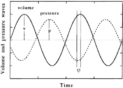
FR mechanism consists on periodical changes in a closed system, by lightly varying its volume. Due to the volume variation a pressure function will be obtained. When the system is empty, these functions have the meeting point in the x-axis and their maximum and minimum peaks occur at the same time [12].
8
Figure 1: Pressure variation in presence of a porous material
In this figure both the volume function and the pressure function that is obtained with the porous material are represented. The main variables that must be measured are the lag (or phase variation, φ) and the amplitude variation (attenuation) between the initial pressure fucntion and the one in figure 1 [13].
The phase varies depending on the time that the diffusion and sorption processes take and the amplitude changes in relation to the amount of solid particles that take place in these processes. The main objective of managing these variables is to obtain diffusion and adsorption-desorption constants.
In order to achieve this, Transfer Functions are used, which characterize pressure response of the system [14].
There are two options during this process, either to have diffusion and adsorption independently, or to have them coupled. A summary of each process’s working is explained next:
- Adsorption: Firstly, adsorption-desorption processes are analysed on uniform surfaces. For this process the Langmuir Isotherm is applied. It starts with a mass m of catalyst particles enclosed in an equilibrium volume Ve. The equilibrium volume is the volume of the system minus the volume of the particles (Ve = V – m/ρs), where ρs is the catalyst particles’ density.
9
- Diffusion: Whenever the adsorptive process does not occur, Fick’s equation solves the diffusional transport of a gas in the porous material’s volume.
- Coupled processes: In this case, both processes occur at the same time so that they affect two different zones of the porous material: Diffusion invades the pore voids and adsorption invades the solid surface. The studying of this process depends on both the fluid and the solid porous material. Depending on the pores and the particles dimension, diffusion and adsorption rates will be comparable or not.
When they are comparable, pores are large in relation to molecular sizes but small enough to provide a big adsorbing area and the constants can be calculated. But when dimensions of cavities are similar to those of diffusing molecules the distinction between gas and adsorbed species cannot be made because the molecules are influenced by the confining surfaces.
10
4 Experimental setup
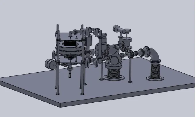
The actual experiment consists on gaskets, connecting pipes, joints, screws, nuts, several types of valves (like bellow valves), fasteners, a vacuum pump, a pressure measuring unit for vacuum, a differential pressure-measuring head, a glass reactor, a volume-modulation unit and two electromagnets.
Figure 2: Complete experimental setup
From the entire set, two parts will be described and analysed in this project. These are: Glass reactor and volume-modulation unit. They are connected by metal pipes through which the fluid flows.
The reactor is made of glass, which has a much smaller conductivity than steel. It is isolated so that the temperature maintains constant.
11
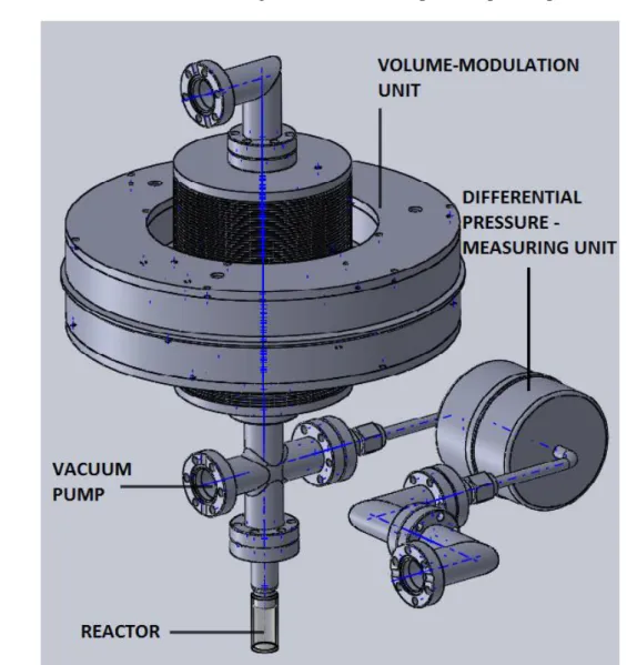
Some other parts are not included in this model, but they are very important on the experiment, and some decisions will be taken depending on their characteristics:
The differential pressure-measuring unit is a device which measures the gauge pressure inside the experiment. It requires a very exact measurement because changes in pressure are relatively small. It also must have a high measuring frequency, as the movement of the bellows is rather fast. Before the experiment starts both sides are equalized so that each measuring consists on a comparison between the new pressure of the system and the initial one.
The vacuum pump is used to evacuate the container and to clean the reactor and the catalyst before inserting again the nitrogen.
The vacuum tubes and blocking valves are used to protect specific parts.
12
13
5 Computational setup
The experiment requires the analysis of the behavior of fluids, when compression-expansion processes occur, and of the heat exchange between these fluids and their surroundings. It also involves he measurement of several variables, as temperature, velocity, pressure or density.
In order to imitate the real volume variation that the FR apparatus generates a vertical movement must be applied to the model.
These problems can be solved using a software called COMSOL Multiphysics (4.4), which is a tool that can describe quite accurately the processes mentioned previously. Three main interfaces will be used: “Moving mesh”, “Laminar Flow” and “Heat Transfer”. These will be customized to represent as precisely as possible the experiment’s main characteristics and constraints.
5.1 Represented components in COMSOL Multiphysics
One of the main benefits of working with this software is that the model’s working variables can be changed at any time, without modifying the entire model. This can be achieved by parameterizing these variables. Every measurement that was taken from SolidWorks will be parameterized as well as the initial fluid conditions and the function parameters.
As it was said before, the two main parts of the entire experiment that will appear in this study will be the volume-modulation unit and the reactor, along with several joining parts such as pipes and rings. This table shows the parameters that have been used to describe each component.
Table 1: List of parameters inserted in COMSOLl Multiphysics
Parameter Value Description
w_glass 1 mm Wall width of glass reactor
d_in1 11 mm Internal diameter of reactor
d_in2 10.4 mm Internal diameter of first pipe and ring
w_pipe1 1.3 mm Wall width first pipe
len1 30 mm Length of glass reactor
len2 24.1 mm Length of first pipe
hei_ring 7.6 mm Height of every ring
w_ring1 11.8 mm Wall width of ring 1
d_in3 16 mm Internal diameter of ring 2
w_ring2 9 mm Wall width of ring 2
w_balg1 36 mm Wall width of top part of bellow
balg_in 46 mm Internal diameter bellow
14
len5 8 mm Length joining part of bellow
d_in_balg 16 mm Internal diameter starting point of
bellow
len3 60.8 mm Length of bigger pipe
num_fin 27 Number of fins per bellow
len_balg_tot 99 mm Maximum length of bellow
len_comp 3 mm Length of compression
w_pipe2 1.5 mm Wall width of bigger pipe
len6 2 mm Length of the joining plate
len_balg 40.5 mm Height of each balg
len_fin 21 mm Length of each fin
w_joiner 46 mm Width of joining plate
max_mov 3 mm Maximum movement of the bellow
freq 10 Hz Frequency of square waves
t_step (0.01/freq) s Step time
P_amb 101325 Pa Pressure of the surroundings
T_amb 298.15 K Temperature of the surroundings
P_N2 133 Pa Pressure nitrogen
5.2 Simulation of the FR system
The FR system is in charge of the movement of the fluid and, consequently, of the heat exchange that will appear in the experiment. Therefore, it is important to represent closely how does it work.
To achieve this, a periodical function is created. There are two preferable options for this purpose: Sinusoidal and square functions.
The choosing criterion will be based on the similarities with the real experiment and the quality of the results. According to this, the sinusoidal function is better managed by the software due to the slow growth of its velocity, but the square function is more easily created, it represents better the actual bellow movement and when it is used, the system has got better long term reliability (f). Hence a square function will describe the FR apparatus movement.
The steps to create this function in COMSOL are: Component 1Definitions (right click)
15 Figure 4: Main parameters of the function that describes the movement
The angular frequency ω of the wave will be 2πfreq, where freq is, as shown on the parameters list, 10Hz. The frequency range of the experiment varies from 0.001 to 10Hz and the latter value is selected because it implies the shortest simulation time with acceptable results.
The phase has a value of π/2 so that the system has its maximum volume at t=0. Both compression and expansion have a duration of 0.01s. Compression starts at t=0.02s and expansion at t=0.07s.
The amplitude is defined as the distance between the middle point of the function and the further point (lowest or highest point). As max_mov is the total displacement of the bellow, the amplitude will be half of its value.
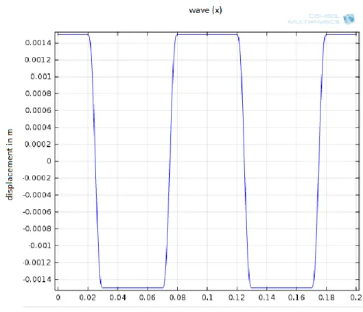
A transition zone is needed so that the square function does not lead to infinite values. Its value will be 10*t_step. The parameter t_step depends on the frequency according to the expression t_step = 0.01/freq (s). This means that if the frequency changes its value, the time step and the transition zone will also vary.
16
Figure 5: Displacement function of the bellows, wave (x)
17
In the velocity graphic it can be seen that a relatively high velocity is reached in a short time and the program takes a long time to solve this. One procedure to avoid this is to increase the transition zone so that the velocity peak is not as sharp, so instead of 10*t_step, 20*t_step and
18
6 Simulations and interface settings
6.1 Geometry
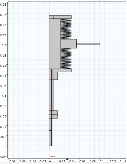
The model is axisymmetric so the geometry is created in a 2D layout, and just the right half of the section is drawn, with the axis on the left-hand side.
All the parts are already modelled in SolidWorks, but as they cannot be imported directly they must be drawn directly in COMSOL. Hence, for each component in SolidWorks, as well as for the entire setup, a section is done so that the measures can be written down. Next figure shows the setup’s section as it appears in SolidWorks.
19
For the model in COMSOL the cross joint is obviated because it just involves the pressure-measuring unit, and it does not affect the results of the experiment. The reactor and the lower pipe have the same diameter as well as every ring that is used for connecting and sealing pipes. The top part, involving two rings and the vacuum pump pipe are not included in the model either. There is a green silhouette around the section that appears in the model.
The geometry is started by drawing rectangles for every domain that the model contains. Click right-button on “Geometry” and “Rectangle” is selected. The domains below the volume-modulation unit are also divided into several rectangles so that no rectangle vertexes appear inside the geometry. This process is done for meshing purposes: It avoids convergence problems and a more regular mesh is achieved.
Afterwards the two bellows are drawn. The chosen option is to use “Polygon”, in which at least three coordinates must be inserted. Just the coordinates of the first fin are typed in. Later, the option “Array” is chosen. It creates a series of copies of the selected geometry. The number of copies the array type (linear or rectangular) and the total displacement can be selected. The total number of fins per bellow is 27. The same procedure is repeated on the upper bellow.
20
In order to measure the change in temperature in this experiment an interface called “Heat transfer” must be used. It only works if there is an outer fluid the experiment is in contact with. Therefore, an air domain must be added to the right of the model.
This air domain has a thickness of approximately 1 cm – it is just an auxiliary domain so its size is not important as long as there is enough space for the fluid properties to develop – and it is set all around the experiment’s outer boundaries.
It is divided in two parts: The lower part that remains still and the upper part which is in contact with the moving part of the setup (volume-modulation unit). By doing it this way it is easier to mesh the domains according to their characteristics.
21
Finally, the option “Form Union” must be chosen in the geometry menu. It joins together all the parts that have been created, facilitating the interface working.
6.2 Materials
In this section the different materials that take part in the experiment will be described and added. In order for the software to operate and calculate the different variables that take place in the process, each domain must be correctly defined by adding a material to it, along with its properties. There are four different materials:
The fluid which flows inside the experiment is nitrogen. In order to choose it, click right-button on “Materials” tab and choose Add Material Liquids and gases Gases Nitrogen. Its main properties are already included, such as density or heat capacity. Although N2 was finally set as main working fluid, CO2 could also be chosen to develop this experiment. As we are working with COMSOL, it is easy to change from one material to the other one if needed.
Next added material is the steel. For the solid parts of the experiment such as pipes and rings, steel AISI 4340 is used. If, in the future, any other kind of steel such as stainless steel is needed, it can be created by clicking “New material” instead of “Add material”. It can be renamed and every property can be added by writing its value/function.
The reactor wall is made of glass, so it will be added to the material list: Add Material Liquids and gases Build-In Glass (quartz).
Lastly, the external fluid is added. The outer domain is simulating the surroundings, this is, the lab. So air is chosen: Add Material Liquids and gases Gases Air.
22
Figure 10: Diagram of the materials used for the model
6.3 Description of the interfaces
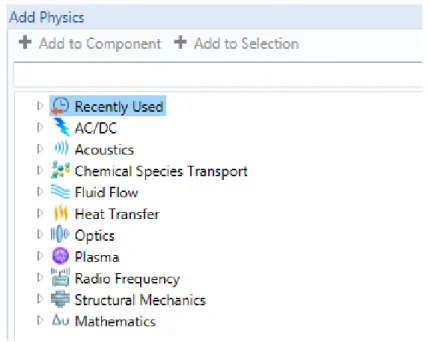
23
All these interfaces can be found by clicking on “Add Physics”. They are divided in different sections according to each science field. The next figure shows this menu and every available field.
Figure 11: “Add physics” menu
This model requires three different interfaces that are described next.
6.3.1 Moving mesh
Moving mesh (ale) is located in the mathematics section and is in charge of the movement of the model. For adding it to the model: Add physics Mathematics Deformed Mesh Moving Mesh (ale). The other interfaces depend on the moving mesh and the movement that it develops to work properly. The function that was created in the computational setup section is used in this interface.
Once the interface is open, the moving part must be selected. This consists on the volume-modulation unit – inner space, bellows, and solid parts – and the upper air domain. The rest of the set will remain still, but the fluid will also be affected by the movement in those parts.
By default just a “Fixed Mesh” and a “Prescribed Mesh Displacement” nodes appear. By right-clicking the ale interface a “Free Deformation” node needs to be opened. The moving domains must be selected here, in order to let the program know that these are the parts that move.
24
wall is 3 mm, the term -0.0015 is added to the function so that the function varies between 0 and -3mm.
Figure 12: Boundary displacement that generates the movement
25 Figure 13: Axis is set to zero horizontal movement
26
“Deformed geometry” is another interface that also works with mesh deformation and that was rejected from this project at the beginning. While “Moving Mesh” implies a deformation of the spatial frame in relation to the material frame, “Deformed Geometry” implies that the material frame is displaced relative to the geometry frame. This makes that in the latter interface the program interprets a volume change that it does not interpret in the former one.
This is another reason for adding the air domain in the geometry section: The “Moving Mesh” interface maintains the entire volume constant, but it allows a volume variation in each separate part.
This interface works with the spatial frame, as it has been said, and its coordinates are z and r. This means that the displacement is measured following these coordinates, and the velocity will be their first derivate, which is zt and rt, according to the software internal language. These velocity terms are the connection that is needed between interfaces.
6.3.2 Laminar flow 1
This interface (spf) is in charge of the management of fluids, the interactions with their surroundings and the calculation of their properties. It can be reached by: Add physics Fluid Flow Single-Phase Flow Laminar Flow (spf). This interface computes pressure and velocity for the single-phase fluid and supports both incompressible and compressible flows at low Mach numbers, as well as non-Newtonian fluids. The equations that the interface uses are the Navier-Stokes equations for the conservation of the momentum and the continuity equation for the mass conservation [10]:
[ ] (Eq.21) (Eq.22)
Both fluids will have different starting densities, so a list of variables is created in order to have a shortcut.
Table 2: Density values used in the model
Variable Expression Description
rho_ref1 mat2.def.rho(P_N2[1/Pa],T_amb[1/K])[kg/m3] Ref. density nitrogen
27
As there are two different fluids and each one has different properties, two different “Laminar Flow” interfaces must be used. The interface that involves and contains the nitrogen is described next.
The default nodes that appear are “Fluid Properties”, “Wall”, “Axial Symmetry” and “Initial Values”. In “Fluid Properties” temperature, pressure, density and dynamic viscosity are selected. In the temperature field, “ht” is set, which matches the fluid interface with the heat transfer interface. The absolute pressure is set as the pressure that corresponds to nitrogen and the reference pressure at 1 atmosphere.
In the node “Initial Values” a velocity field and a pressure are required. The velocity is zero but the pressure does not remain constant because of gravity. The initial pressure inside the cell is 133 Pa, so the entire expression is “P_N2 - P_amb - g_const * (rho_ref1) * z”, where
P_N2 and P_amb are the pressures of the nitrogen and the surroundings, respectively, g_const
is the gravity constant and z is the vertical coordinate. This field requires a gauge pressure.
28
Figure 15: Example of the linear extrusion function
29 Figure 16: Selection of velocity for the wall node
This process is repeated for every boundary which is in contact with the nitrogen and belongs to the area affected by the “Moving Mesh”, so the fluid velocity is as exact as possible.
Next step is to apply the gravity conditions to the experiment. There are three kinds of nodes in every physics tab: Boundary nodes – like those used for adding velocity to the walls –, domain nodes, which are applied to a surface and point nodes. The addition of gravity requires a domain constraint. So by right-clicking on “Laminar Fluid”, a node called “Volume Force” is selected. The unit is N/m3because the programs itself gets the total volume, so the expression written in the “z” field is “-g_const*(spf.rho)”, where spf.rho is the name of the variable the program uses for the nitrogen’s density.
A “Pressure Point Constraint” is added at the bottom right vertex of the nitrogen domain. Its value, also in gauge pressure, is P_N2-P_amb. This process is commonly done in models that use fluid interfaces in order to get a first value that helps the solver getting a solution faster and more efficiently.
30
6.3.3 Laminar flow 2
This interface involves the air domain that simulates the surroundings of the experiment. The default nodes are the same as in “Laminar Flow 1”. The temperature is connected to the heat transfer interface and the pressure is set as the air pressure, with a reference pressure of 1 atm.
In the node “Initial Values” the pressure is set as “–g_const*(rho.ref2)*z”.
In this case, the surroundings pressure does not appear because, as this field requires relative pressure, it is sufficient to write down the pressure variation due to the gravity force.
The external walls of the air domain should simulate the lab conditions. For this purpose a node called “Open Boundary” is selected by right-clicking the “Fluid Flow” node. It is a boundary constraint used for boundaries in contact with large volumes of fluid. The outer walls are selected, except the bottom left boundary, which belongs to the glass reactor and is isolated. The imposed boundary constraint is Normal stress and the value remains at 0 N/m2. Next figure shows this:
31
For the connection between “Moving Mesh” and “Fluid Flow 2”, the same process is repeated, even adding “Wall” to the boundaries that belong to both fluids and to which the velocity has already been established. This is required because they are two different interfaces and they work separately.
After bonding velocities, the gravity is set in the outer domain. Another “Volume Force” node is selected in which the expression now is “–g_const*(spf2.rho)”, where spf2.rho is the air’s
density.
Finally, a “Pressure Point Constraint” is added for converging purposes and to help the solver with the resolution. It is set at the top right part of the air domain and its value is 0 Pa, (the node requires gauge pressure) because the surroundings are at atmospheric pressure.
The “Laminar Flow” part of the study is the most complex one. It involves several fluid properties, and the calculations need a high computational cost. As there are two different interfaces, one for each fluid, the simulation time will increase notably. Also, the bellows have a dense and complex geometry and represent the most likely area for heat transfer.
6.3.4 Heat Transfer
The interface “Heat Transfer in Solids” (ht) is used to model the heat exchange by conduction, convection and radiation although just the two first processes will occur in this model. It uses the differential form of Fourier’s Law, where the temperature is the variable that is needed to be found by using the fluid’s properties and the results from previous interfaces. This equation has been used in section 3 (Eq.18, view page 6) [10].
For this interface the entire geometry is selected, as this process occurs in every component. Both solids and fluids can be analysed by using this interface.
The nodes that are set by default are “Heat Transfer in Solids”, “Thermal Insulation” and “Initial Values”. For the “Heat Transfer in Solids” node, the steel and glass components are selected and the absolute pressure is set to 1atm. For the properties regarding the solids, from material is selected in every term so that the program select the correct properties from each solid.
32
Up to this moment just the solid parts have been selected. In order to include the fluids in our studies, another node called “Heat Transfer in Fluids” must be added. As there are two fluids, two nodes are required. In each one, each fluid’s domains, velocity and pressure must be selected. This node is important for matching both fluid and heat transfer interfaces.
The last two terms of Equation 18 are the viscous heating and the pressure work. Both of these processes are found in this interface, by right-clicking on “Heat Transfer in Fluids”. For the “Viscous Heating” node the pressure and dynamic viscosity of each fluid is selected. The equation that it uses is Equation 20 (view page 7).
The “Pressure Work” node affects the same domains that “Viscous Heating” and represents the heat which is generated from the compression of the fluid and its velocity. It uses Equation 19 (view page 6).
It must be decided whether or not to use the full formulation or the low Mach number formulation – which deletes the last term, which depends on the fluid velocity. As the Mach number – relation between the fluid velocity and velocity of sound in the same medium – cannot be known at this stage, the full formulation is used. Nevertheless, the full equation will always provide more complete information.
The geometry of the bellows makes that both fluids are in contact because they do not have a wall or width. This representation is not correct according to the real experiment. Therefore, another node named “Thin Thermally Layer” is used to define the thickness and thermal conductivity of the resistive material that stands between both fluids. This material is defined by its thermal resistance:
These two material properties must be inserted. The layer thickness, ds, is 0.2mm and the thermal conductivity, ks, 16W/(m·K) [15].
The heat flux is calculated in this interface by the following formulae:
(Eq.24)
(Eq.25)
The subscripts “u” and “d” mean, respectively, up- and downside of the layer.
33
By assigning these nodes to the “Heat Transfer in Solids” interface, the matching is completed and the temperature and heat fluxes can be calculated from the fluid properties.
6.4 Mesh
Meshing is necessary in every model, because it enables the division of the geometry into small units of simple shapes, which are called mesh elements. This discretization enables the program to analyse the model with detail and is in charge of obtaining a certain continuity in the final results [10].
This model is in 2D so the main shapes that can be used are triangular and quadrilateral mesh elements. The “Mesh” module establishes that no mesh vertex can end at a mesh boundary. This is the reason why the initial geometry was divided into numerous rectangles in section 7.1. Next figure shows the division of the lower domains.
Figure 18: Geometry before and after the domain division
34
Once the geometry is decided it is time to build a consistent mesh. As this geometry is complex for a rectangular mesh – which is quite consistent – a triangular one will be used in most domains.
The non-moving part of the air domain will not suffer a big change, because the majority of the heat and the velocity and pressure variations occur in the upper zone. Therefore, the mesh here is set as “Free Quad”. By right-clicking the “Mesh” module a “Free Quad” can be selected and domain 16 is set. Several options can be selected in each mesh type. The node “Size” lets us modify the element size and calibrate it according to the physics that is been used.
Figure 19: Mesh calibration according to the physics
The option General physics is used for the “Free Quad” because, in this case, a rather large mesh is wanted. The size can be predefined or customized by the user.
35 Extremely coarse is chosen in this subgroup, for the same reason.
Afterwards, the rest of the geometry is meshed. A “Free Triangular” mesh is selected for every domain apart from 16. The mesh type and size must be chosen, in order to optimize the results, which will highly depend on the meshing. Four different triangular mesh settings are tried. Their characteristics and results are shown next.
1. The mesh size is customized to obtain a discretization that adjusts to the model. The new values of the element size parameters are:
Figure 21: Values of size parameters for Mesh 1
The maximum and minimum sizes are the absolute size, in meters, that the mesh elements can have. The maximum element growth rate indicates how larger can an element be in relation to its neighbours. In this case, an element’s size can be twice as large as the previous one. By setting this value the elements can grow faster in bigger areas so that the simulation takes a shorter time. The curvature factor is not selected because there are no curved boundaries. The resolution of narrow regions is set to a scalar number less than 1 (0.5) so that the mesh elements in those regions are not too small and the surrounding elements can grow relatively rapid.
36
finer mesh than before because the resolution of narrow regions has a higher value and there is a more notable variation between the maximum and minimum element sizes.
3. The next mesh that is tried is very similar to the second option, but a new feature is added. By right-clicking in the “Mesh” module the option “Boundary Layers” can be selected. It consists on adding several layers of elements – long, quadrilateral divisions – next to the borders of the selected domains. This node is very useful for models that contain fluids because there can be changes in their properties in a slight space and because near the walls, fluids have specific boundary constraints that must be analysed. The number of layers is set to 4 and the rest of parameters remain as they are by default.
Figure 22: Boundary layer parameters
The inner fluid walls are selected (except from the bellow boundaries) for the boundary layers to be added.
37
same as in options 2 and 3, which implies a finer mesh. This has been done because the results of the air domain were not clearly defined in the graphics.
Also, more boundary layers are added in the bellows – in both sides of the boundary – and in the air walls in contact with the setup. Their parameters are identical as those in option 3. With this process a more detailed interaction between fluids will be achieved. This is shown in next figure.
Figure 23: Boundary layers in both sides of the bellow boundaries
38
Figure 24: Velocity results for the comparison of the different types of mesh
39
The simulation time is also taken into account. The next table shows the length of each simulation until the compression was finished.
Table 3: Simulation time for every mesh type
Option Simulation Time
Mesh 1 34min 30s
Mesh 2 2h 31min 18s
Mesh 3 2h 59min 15s
Mesh 4 4h 5min 30s
The first open is the shortest simulation but the results are not descriptive enough. Option 4 is chosen because the time difference in relation to the previous option is admissible.
When the final mesh is decided the model is complete. The last step to follow is the description of the study.
6.5 Study
This module is used to adjust the settings of the simulation in order to obtain the right results. In other words, the way in which the system works and operates is decided in the study.
The study is divided in two parts: “Stationary study” and “Time-dependent” study.
The stationary study is used when variables do not change over time. It is used for compute the steady flow and pressure fields in “Fluid Flow” and to compute the temperature field at thermal equilibrium in “Heat Transfer”. In this model, variables do change over time. So the main goal of using a “Stationary study” node is to get initial values for the variables that are going to be analysed and calculated. After the stationary solver comes the time-dependant solver. It works with the initial values from the previous solver in order to get faster results and more consistent and reliable values [10].
The “Stationary Study” cannot contain any time-dependant variables. Hence, the “Wall” nodes that belong to the “Fluid Flow” interface need to be disabled from the stationary solver, as they contain variables as rt or zt, which depend on time. To achieve this: Stationary Physics and Variables Selection, select the Modify physics tree and variables for study step
40
The “Time-dependent Study” is in charge of the calculating and storing of the results. In the “Time Dependent” tab several characteristics must be modified. The range of time in which the system will be evaluated can be set in Study settings. In this simulation the range will be (0, 0.002, 0.2), which means that 2 cycles will be analysed and 50 time frames will be saved for each cycle.
In Results while solving a graphic can be activated, which represents a variable while the converging process is carried out. The user can select any variable established in the “Results” node. The most interesting variable in this simulation is temperature, so a 3D Temperature graphic – which appears by default in “Results” – is selected.
In Physics and Variables Selection the “Pressure Point Constraint” in the inner fluid must be disabled. Otherwise one point of the nitrogen fluid would be forced to remain constant during the entire experiment and the real conditions would not be reproduced.
The next characteristics tab, Values of Dependent Variables, is in charge of the connection between studies. In order for this study to be adequately correlated with the “Stationary Study” the Initial Values of variables solved for box is selected and the solution of Study 2, Stationary is chosen.
After adjusting the settings in each study, the “Solver Configurations” must be changed. There is one Solver, which involves both studies. This section manages the computing methods that the program uses to operate with the incoming data and to calculate the variables’ values. For the Stationary Study no variation has to be made, but for the Time-Dependent Study the Time-Stepping needs to be modified. Time stepping is the option that decides how often the program stores data and the initial and maximum step can be changed. If the maximum step is too big the results may not be stored completely or correctly. This happens because the function that has been selected is periodically developed. When the system detects two consecutive points with the same value (for example y=0) it interprets that they are the same point and jumps to the last point. If this happens, the displacement function is no longer periodical for the system and the movement is not correct.
41 Figure 25: Initial and maximum step new values
At this point, the system reads the velocity function taken into account every relevant point and storing the correct data.
As several variables must be analysed, it is easier for the program to evaluate them separately. The method that is set by default is a “Direct” method, which assembles every equation and resolves them together. This is changed to a “Segregated” method, in which variables can be studied separately by using “Segregated Steps”. Each interface’s variables are stored in one step. By default just one “Segregated step” but by right-clicking on “Segregated” more can be added.
42
Figure 26: Features of Segregated Step used for “Laminar Flow” variables
43
7 Results and problems faced
7.1 Obtained results and commentaries
While the simulation is running the main graphic shows how the temperature changes with time. This is useful because if there is any unexpected behaviour, it can be easily spotted and the simulation can be stopped so that time is saved.
An approximated value of the results can be manually calculated. Afterwards they can be compared to those obtained in COMSOL. To do this, equations Eq.14 and Eq.15 are used. If they are equalized the resulting equation is:
( )
( )
The property that is known a priori is the volume variation. In order to obtain it a “Surface Integration” can be selected by clicking Results Derived Values and right-clicking on this node. In the expression box the value 2πr must be inserted because the model is in 2D and it is axisymmetric. As the compression is produced in the range [0.002-0.003] the volume will be analysed from the beginning till t=0.003s.
Table 4: Volume variation of the nitrogen during the compression
Time (s) Volume (m3)
0 3.49627e-4
0.005 3.49627e-4
0.01 3.49627e-4
0.015 3.49627e-4
0.02 3.49622e-4
0.025 3.45254e-4
0.003 3.40882e-4
0.035 3.40882e-4
The temperature and the pressure at the initial state of the setup are known (T1=298,15 K and P1 = 133 Pa) and the heat capacity radio of nitrogen is k=1.4 so their final values can be calculated:
( )
44
( )
( )
The obtained results are T2 = 301.186 K and P2 = 137,8 Pa. These results are just an approximation, as these equations were obtained by a series of assumptions in section 3.1.
The most important region where the properties must be controlled is the glass reactor, the bottom part where the porous material will be placed. Therefore, a comparison is going to be made between the volume-modulation unit and the reactor, as well as other relevant points throughout the setup.
7.1.1 Checking of pressure and temperature values in the model
The average pressure of the nitrogen is obtained and a “Table Graphic” is used to represent the result.
45
It can be observed that the maximum average value is 136.56 Pa and the minimum is 132.86 Pa.The pressure result obtained theoretically was 137.8 Pa which is 1 Pa bigger than this.
The system average temperature variation is obtained during two cycles:
Figure 28: Average temperature in the system
After the compression the temperature decreases gradually but it does not reach the initial value, for which it would need more time. Consequently the expansion starts with a temperature offset and does not reach the same (negative) temperature. When the expansion ends, the temperature does not reach the initial temperature either so the next cycle will be at a lower temperature.
The maximum average temperature variation reached is 0.6538 K in the positive part of the graphic and 0.6316 K in the negative. These results differ from the (301.186 – 298.15 =) 3.036 K that were expected.
46
The pressure graphic obtained with COMSOL is now compared to the isothermal and isentropic cases:
Figure 29: Comparison between different pressure functions
The isentropic pressure is represented in green, and it reaches 137,8 Pa, a value which was calculated before. The isothermal pressure corresponds to the red line and it is a good approximation of the simulation pressure. The main difference can be appreciated at the last part of the compression, where the simulation pressure is slightly higher.
7.1.2 Pressure variation in different points of the setup
Pressure values are obtained as a surface average in three different domains:
1- The volume-modulation main domain.
2- The pipe domain in which the pressure-measuring unit is placed in the actual experiment.
3- The bottom part of the reactor.
47 Table 5: Pressure values for the upper domain
Time (s) Pressure 1st cycle (Pa) Time (s) Pressure 2nd cycle
(Pa)
0 132.99704 0.1 132.98771
0.03 136.55716 0.13 136.55407
0.05 136.42569 0.15 136.42423
0.07 136.41816 0.17 136.41706
0.08 132.86223 0.18 132.86111
0.2 132.9873
Table 6: Pressure values for the pipe domain
Time (s) Pressure 1st cycle (Pa) Time (s) Pressure 2nd cycle
(Pa)
0 132.99853 0.1 132.98914
0.03 136.56687 0.13 136.56355
0.05 136.42726 0.15 136.4258
0.07 136.41968 0.17 136.41858
0.08 132.85574 0.18 132.85479
0.2 132.98873
Table 7: Pressure values for the reactor domain
Time (s) Pressure 1st cycle (Pa) Time (s) Pressure 2nd cycle
(Pa)
0 133 0.1 132.99053
0.03 136.57639 0.13 136.57308
0.07 136.42121 0.17 136.42011
0.08 132.84958 0.18 132.84839
0.2 132.99012
These time values have been selected because they are relevant in our study: At t=0.03, 0.13 the compression has just finished, at t=0.07, 0.17 the expansion is beginning, at t=0.08, 0.18 the expansion has finished and t=0, 0.1, 0.2 correspond to the beginning of a cycle.
48
The proximity to the moving wall affects the pressure in the system, but this variation is neglectable due to the dimensions of the model and the properties of the fluid that is being used.
7.1.3 Temperature comparison between volume-modulation unit and reactor
The temperature variation depending on time, during two cycles, is measured in the reactor domain and the volume-modulation domain. The following graphics show this:
Figure 30: Average temperature at the volume-modulation unit and at the reactor
49
7.1.4 Maximum temperature of the system
The maximum temperatures that system reaches in each cycle are 2.01035 and 1.99742 K and it happens at t=0.028 and t=0.128 in first and second cycle, respectively. Next graphic shows the highest temperatures in the system in relation to the time.
Figure 31: Maximum temperatures reached in the system
The effects of irreversibility can be seen here as well. The highest point of the second cycle has decreased its value in relation to the first one.
50
Figure 32: Temperature variation distribution at points 1 and 2, respectively, from Fig. 31
7.2
Problems faced
- A finer mesh was not possible to develop because the moving mesh makes the geometry vary a lot. Hence, the mesh deforms too much and some mesh elements suffer a great displacement so their shape is modified. If this happens, the simulation is forced to an end. An optimization is needed then, so that the model converges with finer mesh and the results can have more reliability.
52
Figure 34 Variation of pressure in the highest elements of the bellows
53
8. Final conclusions
The pressure results show that this property behaves uniformly in the system, as the slight variations are due to the gravity force. The average pressure is, then, an accurate procedure to describe the system.
The isothermal model is very similar to the actual pressure function, except for the small variation at the end of the compression. Therefore, this model can be used in the future for estimated results.
Temperature can affect the system in two ways: Directly on pressure and indirectly, by influencing the adsorption and desorption processes which have an effect on pressure as well. The variation of temperature due to compression-expansion processes play an important role in the bellow, but not in the reactor, where the variation is low enough to say that it does not affect these sorption processes.
54
9 Bibliography
[1] J. Hao, G. Li, Vol. I Air Pollution Caused by Undustries, Department of Environmental Sciences and Engineering, Tsinghua University, Beijing, China.
[2] M. E. Davis, R. J. Davis, Fundamental of Chemical Reaction Engineering, California Institute of Technology & University of Virginia, USA, 2003.
[3] E. M. Flanigen, R. W. Broach, S. T. Wilson, Zeolites in Industrial Separation and Catalysis, 2010, Chapter 1.
[4] P. K. Kundu, I. M. Cohen, D. R. Dowling, Fluid Mechanics, 5th Edition, 2012.
[5] M. I. Hossain, Volume Swing Frequency Response Method for Determining Mass Transfer Mechanisms in Microporous Adsorbents, University of South Carolina, Columbia, USA, 2014.
[6] D. Pérez, Simulation of pressure behavior in a Frequency Response apparatus to determine diffusion and adsorption in porous materials.
[7] E. Poisson, Statistical Physics I (PHY*3240), Lecture notes, Department of Physics, University of Guelph, Canada, 2000.
[8] T. Al-Shemmeri, Engineering Thermodynamics, Department of Renewable Energy Technology, University of Staffordshire, UK, 2010.
[9] C. Sert, Finite Element Analysis in Thermofluids, Department of Mechanical Engineering, Middle East Technical University, Turkey, 2014.
[10] COMSOL Multihyscs Reference Manual.
[11] A. Costa, G. Macedonio, Viscous heating in fluids with temperature-dependent viscosity: implications for magma flows, University of Natural Sciences of Pisa, Italy, 2003.
[12] S. C. Reyes, E. Iglesia, Frequency Modulation Methods for Diffusion and Adsorption Measurement in Porous Solids, The Journal of Physical Chemistry B, pp 614-622, University of California, California, USA, 1997.
[13] P. F. Deisler Jr., R. H. Wilhelm, Diffusion in Beds of Porous Solids Measurement by Frequency Response Techniques, Princeston University, New Jersey, USA, 1953.
[14] Y. Li, D. Willcox, R. D. González, Determination of Rate Constants by the Frequency Response Method: CO on Pt/SiO, Department of Chemical Engineering, University of Illnois, Chicago, USA, 1989.
55
10. APPENDIX – Symbols
cv Specific heat of nitrogen for constant volume [743 J/kg·K]
cp Specific heat of nitrogen for constant pressure [1040 J/kg·K]
ds Resistive layer thickness [m]
E Total energy [J]
F Volumetric forces in fluid flow [N/m3]
g Gravity constant [9,806 m/s2]
hi Enthalpy for the species i [J/kg]
I Unitary matrix
ks Thermal conductivity of bellows [W/(m·K)]
k Heat capacity ratio of nitrogen [1.4]
ksteel Conductivity of the steel [44.5 W/(m·K)]
m Mass [kg]
ṁi Mass flow rate of the species i [kg/s]
Pn Pressure at the n state of the process [Pa]
P Pressure of gas [Pa]
pA Absolute pressure of gas [Pa]
External heat sources [J]
Total heat [J]
̇ Heat power [W]
R Ideal gas constant for nitrogen [296,8 J/kg·K]
Rs Thermal resistance [m2·K/W]
S Total entropy [J/K]
Ṡq Entropy variation due to heat conduction [J/K·s]
Ṡirr Entropy variation due to irreversibility [J/K·s]
56
T Temperature of fluid [K]
Tn Temperature at the n state of the process [m3]
t Time [s]
U Internal energy [J]
ui Fluid velocity [m/s]
V Volume [m3]
Ve Equilibrium volume in adsorption processes [m3]
Vn Volume at the n state of the process [m3]
W Work [J]
Ẇ Work power [W]
Wp Pressure work [J]
zi Height [m]
µ Dynamic viscosity [Pa·s]
ρ Gas density [kg/m3]
ρs Density of adsorptive particles [kg/m3]
φ Phase lag [rad]
Φ Viscous heating term [J]