Abstract
Commercial laminated glass is usually composed of two glass layers and an interlayer of PVB. The viscoelastic behaviour of the PVB layer has to be taken into account when dealing with dynamic loads. This paper shows different Finite Element (FE) models developed to characterize laminated glass. Results are contrasted with data from different reference test cases. First, a quasi-static test is reproduced with a 2d model through a transient analysis. In addition, flexural modes of vibration in a free-free test configuration have been analysed using 2d as well as 3d FE models. Apart from using transient analysis in order to simulate the dynamic behaviour of laminated glass, an iterative procedure has been employed which permits to identify the correct value of the shear modulus of the PVB layer for each mode in an eigenvalue analysis.
Keywords: laminated glass, viscoelasticity, temperature dependency, frequency dependency, simplified numerical models, iterative modal identification, PVB.
1 Introduction
As a result of its increasing importance, many improvements have been made since laminated glass was invented. Its increasing popularity comes from its multiple uses as it can be applied for many safety and security needs, varying only its thickness. Commercial samples are usually composed of two or more glass layers with a thickness of either 2.9 mm or 3.8 mm and an interlayer of polyvynil butiral (PVB from now on) 0.38 mm thick, but more layers can be added to produce stronger glass. While commercial thicknesses can be sufficient for many applications such as curtain walls or windshields, additional layers of PVB and glass are used to obtain the increased strength needed for bulletproof products.
Thus, it turns out to be necessary to model this composite material with such interesting characteristics for human safety and security for design purposes [1].
Paper
253
Comparison of Different Finite Element Models for the
Transient Dynamic Analysis of
Laminated Glass for Structural Applications
J. Barredo1, M. Soriano2, L. Hermanns2, A. Fraile2 M. López3 and M.S. Gómez2 1 Centre for Modelling in Mechanical Engineering (CEMIM-F2I2)
2 Department of Structural Mechanics and Industrial Constructions
Polytechnical University of Madrid, Spain
3 University of Oviedo, Gijón, Spain
©Civil-Comp Press, 2010
While the static behaviour is well understood and several design codes like [2] are available, the dynamic response of laminated glass is an important research topic due to its complex nature. In the context of dynamic analysis glass can be considered as a linear elastic material while PVB is considered to behave viscoelastically. The time dependent viscoelastic properties imply transient dynamic analyses in order to represent stress relaxation and creep. The PVB layer is generally almost ten times thinner than the glass layers leading to finer meshes so as to obtain well-shaped elements. Hence, models become more intricate and calculation times increase notoriously.
2 Objective
The computer time needed to run 3D models is very large and consequently their use is normally limited to benchmark studies. For this reason these models are impractical for parametric studies even though they return reliable results that agree with those from different reference test cases.
Therefore, the paper’s main objective is to represent the mechanical behaviour of laminated glass subjected to dynamic loads with simplified models that return results of reasonable accuracy but requiring shorter simulation times. A comparison will be made throughout the paper between the different models proposed.
3 Material characterisation
3.1 Glass characterisation
Even though there are many different types of glass, it may be considered a homogeneous, isotropic and linear elastic material within the range of time scales and temperatures considered throughout this paper. The most important properties of the particular type of plane glass used in the benchmark cases are listed in Table 1.
Young’s modulus Poisson’s ratio Density E=72 GPa ν=0.22 ρ=2500 kg/m3
Table 1: Glass properties
3.2 PVB characterisation
PVB is both time and temperature dependent; thus, it is considered as a linear viscoelastic material. The time-dependent response is characterised by separated volumetric and deviatory terms, being the first characterised by the bulk modulus K
( )
(
)
( )
2(
)
( )
t t
d
d d
t K t d G t d
d d
ν τ τ
σ τ τ τ τ
τ τ
−∞ −∞
=
∫
− ε +∫
− ε (1)The bulk modulus of PVB is considered to be constant throughout this study. The shear modulus can be represented by a Prony series as shown in equation (2).
( )
01
G G
i
n
G G
i i
G G e
τ τ
τ α∞ α −
=
⎡ ⎤
= ⎢ + ⎥
⎢ ⎥
⎣
∑
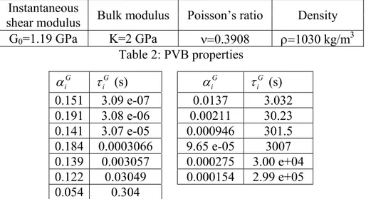
⎦ (2)More information about the modelling of viscoelastic material behaviour can be found in standard text books like [3],[4],[5],[6] and [7]. Parameters of the Prony series have been obtained by means of testing PVB material. Since the bulk modulus is considered constant, the test has been carried out to determine the Prony series parameters of Young’s modulus E and making the necessary transformations to determine the corresponding values of the shear modulus. The tests have been carried out at the reference temperature of 20ºC. Results are shown in Table 2 and 3.
Instantaneous
shear modulus Bulk modulus Poisson’s ratio Density G0=1.19 GPa K=2 GPa ν=0.3908 ρ=1030 kg/m3
Table 2: PVB properties
G i
α G
i
τ (s) αiG
G i τ (s) 0.151 3.09 e-07 0.0137 3.032 0.191 3.08 e-06 0.00211 30.23 0.141 3.07 e-05 0.000946 301.5 0.184 0.0003066 9.65 e-05 3007 0.139 0.003057 0.000275 3.00 e+04 0.122 0.03049 0.000154 2.99 e+05 0.054 0.304
Table 3: Prony series parameters at a reference temperature of 20ºC
Temperature dependence has been characterised using one of the most commonly used shift functions: the Williams-Landel-Ferry shift function (WLF from now on), which is shown in Equation (3) [3]. WLF constants are given in Table 4.
( )
1(
)
10
2
log ref
ref
C T T A T
C T T
− ⎡ ⎤ = −
⎣ ⎦ + − (3)
WLF constants
C1 C2 Tref
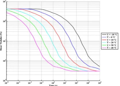
Time and frequency dependency of the shear modulus is represented in Figures 1 and 2, respectively.
Figure 1: Shear modulus vs. time at different temperatures
Figure 2: Shear modulus vs. frequency at different temperatures
4 Quasi-static analysis
prepared and the behaviour of the PVB and the glass has been compared with the test results.
In what follows, the tests and the model are described in detail.
4.1 Test description
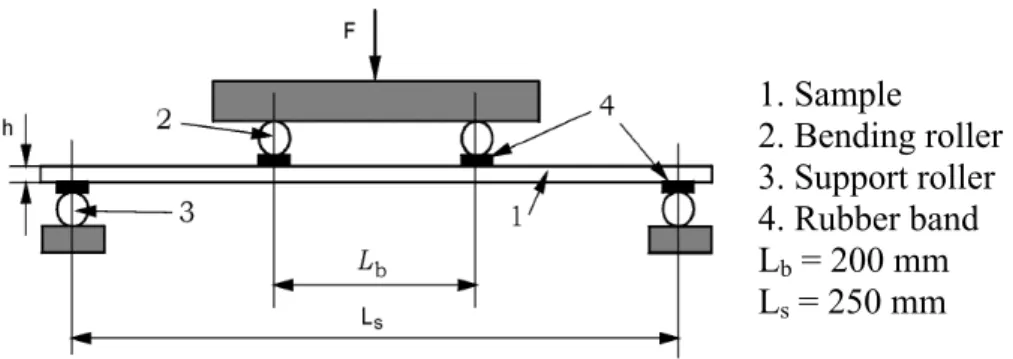
A four point bending test has been carried out on a 8mm thick laminated safety glass sample with a 0.76mm PVB layer, 100mm wide and 300mm long. A similar test setup as the one proposed by European Standard EN 1288-1:2000 [7] was used nevertheless this Standard refers to plane monolithic glass. On Figures 3 and 4 the way in which the sample has been placed for testing is shown.
1. Sample
2. Bending roller 3. Support roller 4. Rubber band Lb = 200 mm Ls = 250 mm
Figure 3: Four point bending test description
Figure 4: Real test setup
4.2
A p per dim has hei bet 0.6 to sho The lab at a
2 Descrip
plane strain rmits both mensional 8s been used ight of the tween the sa 6 for the fric
avoid conv ows a detail
e calculatio boratory. In a rate of 0.0
Fi
ption of th
n model ha very fine m 8-node plan d. Symmetr plate have ample and t ction coeffic vergence pro
l of the mesh
F on has been
this case, th 016 mm/sec
igure 5: Pos
he plane F
s been emp meshes and ne element ry condition
been chose the support cient has be oblems, the h near the c
igure 6: De n carried ou
he temperat ond.
sition of the
Finite Ele
ployed to si d reduced c
that exhibi ns have bee en using thr t rollers has een employe e mesh is f contact poin
etail of the c ut taken int ture was 22
e strain gaug
ement mo
imulate the calculation t
ts quadratic en applied. ree element s been taken ed according finer near th nts.
contact regio to account 2ºC and the
ges
odel
e test. This times. A h c displacem
Nine elem ts for each n into accou g to the liter he contact z
on
the test con displaceme
type of mo igh-order tw ment behavi ments along
layer. Con unt. A value
rature. In or zone. Figur
nditions in ent was app
4.3
The mo cal the An num dis Co Res com The lay at t Str ain ( μ m/ m ) Str ain ( μ m/ m )3 Results
e load-disp odel is compibration pro e numerical
n initial pre merical mod
placement c mparison in sults obtain mpared.
e stress dist yers behave their respec
s compar
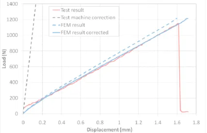
placement c pared in Fig ocess. The a results befo
Fi eload was del since th curve. n terms of l ned from t
tribution in almost like ctive tops an
ison
curve obtain gure 7. The additional d ore compari
igure 7: Loa imposed in he main obje load vs stra the test and
Figure 8: the centre e two separa nd under tra
ned from t stiffness of displacemen ing experim
ad vs. displa n the test. ective consi ain avoids in
d the nume
Strain vs. lo section of t ated plates. action at the
St ra in ( μ m/ m ) St ra in ( μ m/ m )
the test ma f the test m nts during th mental and n
acement cur This effec ists in match ntroducing t
erical mode
oad curves the sample
Both of the eir bottoms.
achine and machine is de he test have numerical re
rve
ct is not re hing the slo the test mac els may th
reveals tha em are unde . The stress
the numer etermined b e been added esults.
eflected in ope of the lo chine stiffn hus be dire
the lay app
Sin sati mo
5
5.1
For spe wit
Ch
e PVB layer yers i.e. its
preciated in
Figu nce the mo isfactory, th ore sophistic
Moda
1 Test de
r the moda ecimen was th a pen in t
aracteristics
r is determi top is und Figure 9.
ure 9: Stress odel behave he next step cated test.
al identif
escription
al identifica s supported time, space
Fi s of the sam
ned by the der traction
s distributio es quite we p taken con
fication
n
ation, a free by means and intensit
igure 10: Fr mple are deta
boundary v n while the
n along the ell and the
sists in usin
e-free test of two stri ty. Figure 1
ree-free test ailed in Tab
values at the e bottom is
height of th e agreement ng this simp
case has b ings and ha
0 illustrates
configurati ble 5.
e interfaces s compress
he test spec t with the plified mod
een carried as been ran s the tested
ion
s with the g ed as may
imen test results del to analyz
d out. The ndomly exc configurati
lass y be
s is ze a
Length (mm) Width (mm) Thickness (mm) Accelerometers
500 100 3+0.38+3 6
Table 5: Sample characteristics
The six accelerometers have been equidistantly spaced along the centre line of the test specimen, thus allowing only identification of bending modes.
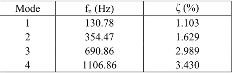
Mean results from several tests employing the stochastic subspace identification method (SSI) are condensed in Table 6.
Mode fn (Hz) ζ (%)
1 130.78 1.103 2 354.47 1.629 3 690.86 2.989 4 1106.86 3.430 Table 6: Results obtained with the SSI method
5.2 Iterative modal identification
As a first approach for modal identification, an iterative procedure has been applied taking into account the frequency dependency of PVB’s shear modulus. The value of the shear modulus is chosen for each target modal frequency. Afterwards, a finite element modal analysis is done and the corresponding modal frequency of interest is compared to the one for which the shear modulus had been chosen. If the absolute difference between both of them is greater than 10-3 Hz, the shear modulus is readjusted. The process is then repeated for each mode and sample. The flow chart on Figure 11 will clarify the process.
Figure 11: Iterative modal identification flow chart
Consequent to the process, simulation times need to be small enough to make the iterative modal identification feasible. As a result, a three-dimensional solid model with a coarse mesh has been employed.
A high order three-dimensional 20-node solid element that exhibits quadratic displacement behaviour is chosen. Each node has three degrees of freedom: translations in the nodal directions x, y and z.
In order to model the two strings that support the sample, a uniaxial tension-only three-dimensional spar element is selected. With the tension-only option, the stiffness is removed during transient dynamic analyses if the element goes into compression. To represent the influence of the accelerometers, structural masses are used. The geometry and imposed boundary conditions are illustrated in Figure 12.
Figure 12: Geometry and boundary conditions of the 3d solid model
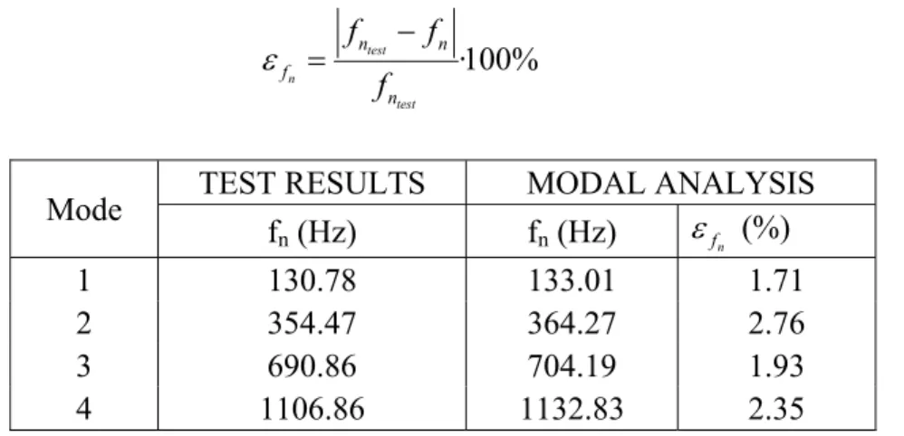
Results comparison in terms of natural frequencies is shown in Table 7. The relative difference εfn between experimental and numerical results regarding the natural frequency is defined in Equation (4).
·100%
test n
test
n n
f
n
f f
f
ε = − (4)
Mode TEST RESULTS MODAL ANALYSIS
fn (Hz) fn (Hz) εfn (%)
1 130.78 133.01 1.71
2 354.47 364.27 2.76
3 690.86 704.19 1.93
4 1106.86 1132.83 2.35
Table 7: Comparison of test and modal analysis results
5.3
5.3 Du bee mo The of pla nod To The An res In rea par con To Res sam3 Transi
3.1 Plane m
ue to the goo en used to s odelled and
e model ha each glass ane element de has two d
represent t e geometry
Figu n impulsive
pond enoug order to de ally necessa rametric st nsideration: • Numbe • Numbe frequen
limit the co sults from t me identific
ient dynam
model
od results ob simulate the a soft sprin s been mesh
layer and 3 t that exhib
degrees of f the influenc and impose
ure 13: Geom force has gh time so th etermine wh ary to corr tudy has
er of points
er of cycles ncy. omputationa this paramet ation algori
mic analy
btained for e modal tes g has been hed with 10 3 for the PV bits quadratifreedom: tra ce of the ac
ed boundary
metry and b been applie hat both dam hat does en rectly ident been reali
necessary t
n=
s during the
m=
al effort onl tric study ar ithm as in th
ysis
the quasi-st st. As the s
added. 00 elements VB layer. A ic displacem anslations in
celerometer y conditions
boundary co ed and then mping and n nough time
tify both d ised. Two
to describe t 1 · max t f = Δ e simulation · min max f t =
ly the first m re gathered he test case
tatic simula trings are p s along the A high order
ment behav n the nodal rs, structura s are illustra
onditions of n the samp natural freq exactly me damping an variables the highest n correspon
mode is con on Figures (SSI).
ations, the pl perpendicul
length, 5 al r two-dimen viour has be
directions x al masses h
ated in Figu
f the plane m le has been quencies can ean and wh nd natural have bee
natural freq
ding to the
nsidered in w 14 and 15,
lane model ar to the pl long the hei nsional 8-n een used. E x and y.
ave been us ure 13.
model n left to fre n be identifi hat time step
frequencies en taken i
In o lea sho val Use hig and cho
Figur
Fig
order to obt ast 30 point ould be used lue is signif
er Manual o ghest mode d natural fr osen as indi
re 14: Param
gure 15: Par
tain results ts. Taking a d when dam ficantly high of Ansys! A frequency requencies icated in Eq
metric study
rametric stud
of reasonab a look at F mping ratios her than the According to
should be the maximu quations (7)
t
Δ =
y for the firs
dy for the fi
ble accuracy Figure 15 it have to be e lower limi
o [9] at leas used. Thus um time st
and (8). 1 30·fmax
=
st mode – N
first mode –
y one cycle t can be se determined t that is stat st 20 discret , to identify tep and min
Natural frequ
Damping r
should be s en that eve d with high ted as rule o
te points pe fy correctly
nimal durat uency
ratio
ampled wit en more po precision. T of thumb in er period of
both damp tion should
th at oints This the f the ping d be
100
max min
t f
= (8)
5.3.2 3d solid model
A more sophisticated model is required in order to validate the simplified one. As has been shown before, the plane model estimates quite correctly the first natural frequency using transient dynamic analysis and with the simplified iterative modal analysis the resulting frequencies of the first four bending modes have been determined with relative differences of less than 3%. While the frequencies may be determined to within acceptable errors, the differences between the obtained damping values are very large. Therefore, a 3d solid model has been employed in order to confirm the damping ratios obtained with the plane model.
The calculation has been focused on the first natural frequency in order to limit computer time. For the same reason the recommended number of cycles has been slightly relaxed to 80 instead of 100. On the other hand the number of time steps per cycle has been chosen to be 60 in order to increase the precision of the identified damping values.
As the study has been focused on the first natural frequency, a symmetric model that considers half of the test specimen is sufficient for the identification.
The model has been meshed with 25 elements along the length and 10 along its width. Three elements have been used along the thickness of each glass layer and one for the PVB layer.
The influence of the accelerometers has been accounted for by including structural masses.
5.4 Results comparison
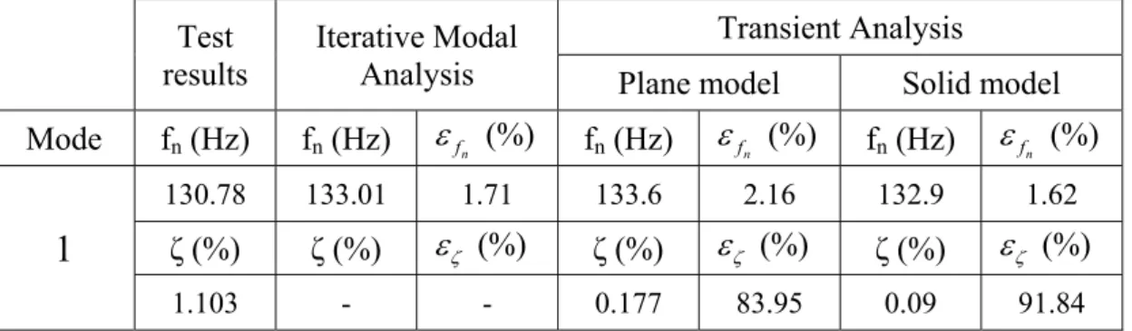
Results obtained from the 2d as well as 3d models for the first mode are presented together with the test results in Table 8.
The relative difference εζ between experimental and numerical results regarding the damping ratio is defined in Equation (9).
·100%
test
test ζ
ζ ζ
ε
ζ
−
Test
results Iterative Modal Analysis
Transient Analysis
Plane model Solid model Mode fn (Hz) fn (Hz) εfn (%) fn (Hz) εfn (%) fn (Hz) εfn (%)
1
130.78 133.01 1.71 133.6 2.16 132.9 1.62
ζ (%) ζ (%) εζ (%) ζ (%) εζ (%) ζ (%) εζ (%)
1.103 - - 0.177 83.95 0.09 91.84
Table 8: Damping ratios identified employing SSI algorithm
The results obtained from the 3d solid model confirm those obtained with the 2d models demonstrating that the simplified models behave in a correct way.
The three methods employed to determine the natural frequencies return acceptable results being the relative difference between experimentally and numerically obtained values always below 3%. However, the damping ratio shows similar differences for both 2d and 3d models with regard to the test results. Therefore, it seems that these models do not reflect adequately the damping mechanisms present during the tests.
Further investigations are being carried out in order to clarify this issue. On one hand, it may be possible that the damping of the glass layers has to be taken into account. On the other hand, it’s also thought that the accelerometer cables introduce some amount of damping which may be important considering the generally low damping ratios. To check this, more tests are going to be carried out eliminating the cables and measuring displacements by means of a laser device.
6 Conclusions
The results obtained show that the 2d models may be used for the identification of bending modes or the simulation of the four point bending test. This is particular interesting when using iterative procedures or performing parametric studies as computer time is crucial in these cases. An iterative procedure has been presented to estimate the natural frequencies taking into account the frequency dependence of the shear modulus of the PVB layer.
To identify damping ratios a free-free test configuration has been used. The test specimen has been excited randomly by a pen and the acceleration time histories have been analysed with the SSI method. The test has been simulated with 2d and 3d models and with both types of models the natural frequencies could be identified with reasonable accuracy. However, a quite big difference exists between experimentally and numerically obtained damping ratios. It is thought that the FE models do not include all the dissipative mechanisms that worked during the tests like for instance the damping of the glass layers or the accelerometer cables. Further studies are necessary to clarify this issue.
Acknowledgements
This work has been made under the sponsorship of the University State Secretary, belonging to Spanish Ministry of Science and Innovation, in its contract BIA2008-06816-C02-02. The presented results have been obtained in cooperation with Universidad de Oviedo.
References
[1] M. A. García Prieto, “Dimensionamiento probabilístico y análisis experimental de vidrios en rotura”. Doctoral thesis, 2001.
[2] ASTM E1300 - 09a Standard Practice for Determining Load Resistance of Glass in Buildings
[3] R.S. Lakes, “Viscoelastic materials”, Cambridge University Press, New York, USA, 2009
[4] R.M. Christensen, “Theory of viscoelasticity”, Dover Publications Inc, New York, USA, 1982.
[5] D.I.G. Jones, “Handbook of viscoelastic vibration damping”, John Wiley & Sons Ltd, West Sussex, England, 2001.
[6] W.N. Findley, J.S. Lai, K. Onaran, “Creep and relaxation of nonlinear viscoelastic materials”, Dover Publications Inc, New York, USA, 1989.
[7] W. Flügge, “Viscoelasticity”, Blaisdell Publishing Company, Waltham, Massachusetts, USA, 1967.
[8] UNE- EN 1288-3:2000 Vidrio para la edificación - Determinación de la resistencia a flexión del vidrio -Parte 3: Ensayos con probetas soportadas en dos puntos (flexión 4 puntos).