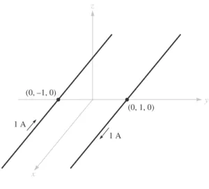
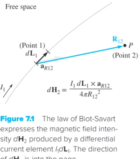
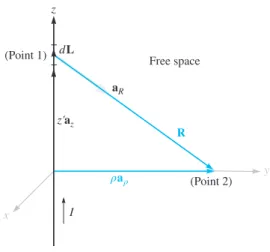
The direction of the magnetic field intensity is perpendicular to the plane containing the differential filament and the line drawn from the filament to the point P. It follows that only the integral form of the Biot–Savart law can be verified experimentally. . We illustrate an application of the Biot-Savart law by considering an infinitely long, straight filament.
One useful result is the field of the finite-length current element, shown in Figure 7.5. The simplest surface is therefore that part of the plane surrounded by the road.

CURL
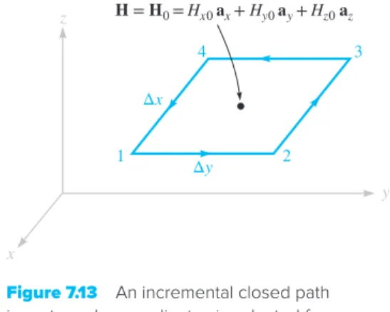
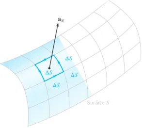
The curl of any vector is a vector, and any component of the curl is given by the limit of the quotient of the closed line integral of the vector around a small path in a plane perpendicular to the desired component and the enclosed region that the path shrinks to zero. The N subscript indicates that the component of the curl is the component normal to the surface enclosed by the closed path. Equation (24) is even more concise and leads to (22) using the definitions of the cross product and vector operator.
Although we have described the curl as a line integral per unit area, this does not provide everyone with a satisfactory physical picture of the nature of the curl operation, because the closed line integral itself requires physical interpretation. No twist means no curl; larger angular velocities mean larger curl values; a reversal in the direction of rotation means a reversal in the sign of the curls. To find the direction of the vector curl and not simply to determine the presence of any particular component, we need to place our paddle wheel in the field and find the orientation that produces the greatest torque.
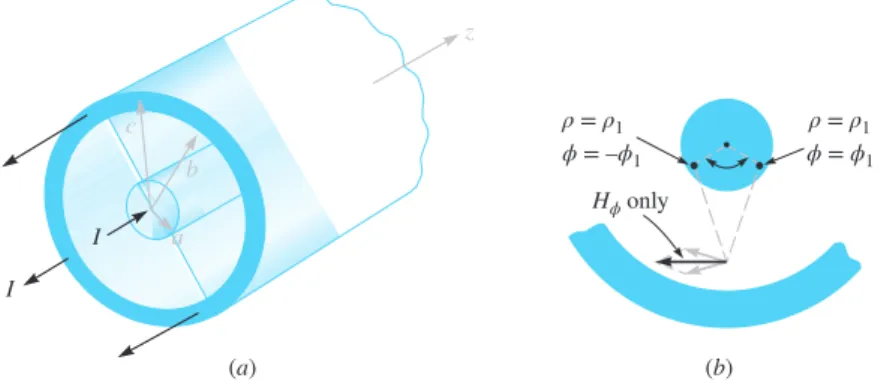
The direction of the curl is then along the axis of the impeller, as indicated by the right-hand rule. Figure 7.14b shows the magnetic field intensity current lines around an infinitely long wire-like conductor. It seems possible that if the curvature of the streamlines is correct and also if the variation of the field strength is just right, the net torque on the impeller can be zero.
Returning now to complete our original investigation of the application of Ampère's circuit law to a differential-magnitude path, we can combine and (24), .
STOKES’ THEOREM
We are given the field H = 6r sin ϕar + 18r sin θ cos ϕaϕ and asked to evaluate each side of Stokes' theorem. The differential path element dL is the vector sum of the three differential lengths of the spherical coordinate system first discussed in Section 1.9. The integral of the current density across the surface S is the total current I passing through the surface, and so.
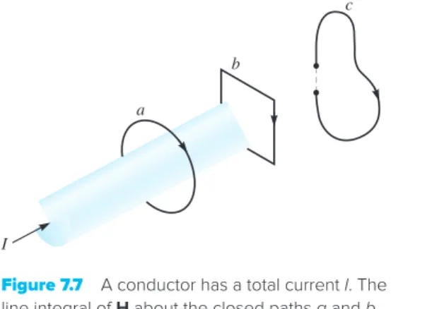
This brief derivation clearly shows that the current I, described as being "closed by the closed path," is also the current passing through any of the infinite number of surfaces that have the closed path as a circumference. The left-hand side is the surface integral of the curl of A over the closed surface surrounding the volume v. Stokes' theorem relates the surface integral of the curl of A over the open surface enclosed by a given closed path.
If we think of the path as the opening of a laundry bag and the open surface as the surface of the bag itself, we see that as we gradually approach a closed surface by pulling on the drawstrings, the closed path becomes smaller and smaller and eventually disappear as the surface closes. Hence, applying Stokes' theorem to a closed surface yields a zero result, and we have. Thus, the results verify Stokes' theorem, and we note in passing that a current of 22.2 A flows upward through this portion of a spherical hood.
We now see that Stokes' theorem enables us to obtain the integral form of Ampère's circuit law from the point form.
MAGNETIC FLUX AND MAGNETIC FLUX DENSITY
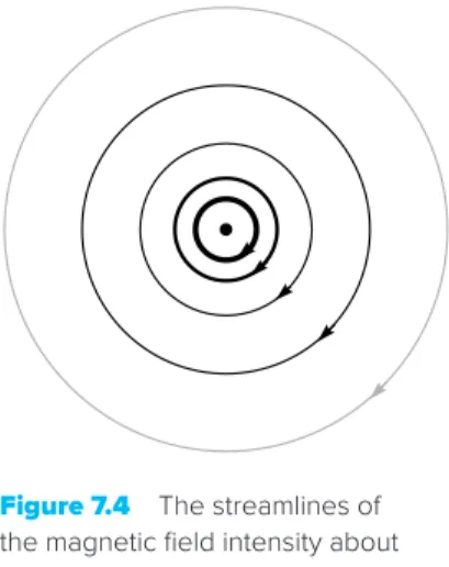
In the example of the infinitely long straight filament carrying a direct current I, the H field formed concentric circles around the filament. The magnetic flux lines are closed and do not terminate on a "magnetic charge". For this reason, Gauss's law for the magnetic field. Equation (36) is the last of Maxwell's four equations as it applies to static electric fields and steady magnetic fields.
To these equations we can add the two expressions relating D to E and B to H in free space. In addition, we extended our coverage of electric fields to include conducting and dielectric materials, and introduced polarization P. Returning to (37), it can be noted that these four equations specify the divergence and curl of an electric and a magnetic field .
Our study of electric and magnetic fields would be much simpler if we could start with one or the other equation (37) or (41). With a good knowledge of vector analysis, as you should now have, either set can be easily obtained from the other using the divergence theorem or Stokes' theorem. As an example of the use of flux and flux density in magnetic fields, find the flux between the conductors of the coaxial line in Figure 7.8a.
The magnetic flux between conductors of length d is the flux that crosses any radial plane that runs from ρ = a to ρ = b and from, say, z = 0 to z = d.
THE SCALAR AND VECTOR MAGNETIC POTENTIALS
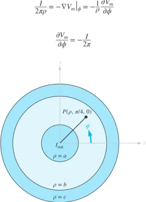
Each time we make another complete circuit around the current, the result of the integration increases by I. This is another facet of the analogy between electric and magnetic fields about which we will have more to say in Chapter 8. Then a vector identity that we proved in section 7.4 shows that the divergence of the curl of each vector field is zero.
The convolution of the vector field is not equal to zero and is given by a rather complicated expression,9 which we do not now need to know in general form. The meaning of the terms in (47) is the same as in the Biot-Savart law; a direct current I flows along a filamentary conductor whose any differential length d L is at a distance R from the point where A is. Since we have defined A only by specifying its coil, the gradient of any scalar field can be added to (47), without changing B or H, since the convolution of the gradient is identical to zero.
The magnitude of the vector magnetic potential varies inversely with the distance to the current element, and is strongest in the vicinity of the current and gradually falls to zero at distant points. Skilling10 describes the vector magnetic potential field as "like the current distribution but blurred around the edges, or like a picture of the current out of focus." Since the size of the filamentary element is constant, we have chosen the form that allows us to remove one quantity from the integral.
Analogous expressions for A will be derived in the next section, and the example calculation of the vector magnetic potential field will be completed.
DERIVATION OF THE STEADY-MAGNETIC- FIELD LAWS
Consequently, it can be factored out of the curl function like any other constant, leaving out. The second term of this integrand is zero because ∇2 × J1 denotes the partial derivatives of a function x1, y1 and z1, taken with respect to the variables x2, y2 and z2; the first set of variables is not a function of the second set, and all partial derivatives are zero. The first term of the integrand can be determined by expressing R12 in terms of coordinate values, .
To find the Laplacian of the vector A, let us compare the x-component of (51) with the similar expression for electrostatic potential. However, we have obtained some additional information about the electrostatic potential that we do not need to repeat now for the x-component of the vector magnetic potential. Finally, let us return to (64) and make use of this formidable second-order vector partial differential equation to find the vector magnetic potential in one simple example.
We select the field between the conductors of a coaxial cable, with rays a and b as usual, and current I in the a-z direction in the inner conductor. We have already been told (and Problem 7.44 gives us the opportunity to check the results ourselves) that the Laplace vector can be expanded as the vector sum of the scalar Laplaceians of the three components in rectangular coordinates. However, it is not difficult to show for cylindrical coordinates that the z-component of the Laplacian vector is the scalar Laplacian of the z-component of A, or.
Equation (66) is obviously also applicable to the exterior of any conductor with a circular cross-section, along which a current I flows in the direction az in free space.

PROBLEMS
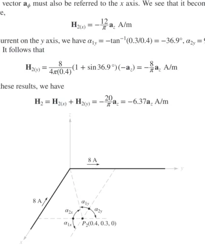
Now consider two conductors, each of radius 1 cm, parallel to the z-axis with their axes lying in the plane x = 0. A surface charge of uniform density ρs lies on the disk, which rotates about the z-axis with angular velocity Ω rad/ s. Apply the Biot-Savart law and find H anywhere on the z-axis; (b) repeat part (a), but with the copper foil occupying the entire plane (Hint: express aϕ in terms of ax and ay.
Is is the current in a circular band of length dz on the coil; the solenoid consists of these bands of current along its entire length. At the origin it connects to a conducting sheet forming the xy plane. a) Find K in the conduction sheet. The current flows as a surface current radially inward on the plane to the vertex of the cone, and then flows radially outward through the cross-section of the conical conductor.
The wire carries a non-uniform current along its length density J = bρ az A/m2 where b is a constant. a) What total current flows in the wire. A solid conductor is in the form of a circular cylinder with its axis along the z-axis. A square filamentary differential current loop, dL on a side, is centered at the origin in the z = 0 plane in free space.
The current I generally flows in the aϕ direction. a) Assuming r ≫ dL, and following a method similar to that in Section 4.7, show.