This helps with the discussion of statistical properties in Chapter 3 as well as the new Chapter 4. This chapter on inference covers confidence intervals and statistical tests of hypotheses, two of the most important concepts in statistical inference.
Introduction
Sometimes called the probability that the outcome of the random experiment is inC; sometimes called the probability of the eventC; and is sometimes called the probability measure of C. One of the most logically satisfying theories of probability is that based on the concepts of sets and set functions.
Set Theory
Note that the number zero is not in this array because it is not in one of the arrays C1, C2, C3,. Many functions used in calculus and in this book are functions that map real numbers to real numbers.
The Probability Set Function
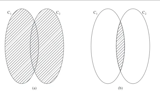
Then consider the probability of the event E2 getting exactly three of a kind, (the other two cards being different and of different kinds). If the probability set function P assigns a probability of 16 to each of the elements of C, computes P(C1),P(C2),P(C1∩C2) and P(C1∪C2).
Conditional Probability and Independence
We want to calculate the probability that the first draw results in a red chip (C1) and that the second draw results in a blue chip (C2). The probability that the third spade appears in the sixth draw is calculated as follows.
Random Variables
On the other hand, if the identity of the random variable is clear, then we often suppress the signatures. The pmf of a discrete random variable and the pdf of a continuous random variable are quite different entities.
Discrete Random Variables
Transformations
Continue to draw chips from the bowl, one at a time and randomly and without replacement, until the red chip is drawn. a) Find the pmf ofX, the number of trials required to draw the red chip. Roll a die a number of independent times until a six appears on the face of the die. a) Find pmfp(x) of X, the number of rolls required to obtain the first six.
Continuous Random Variables
Transformations
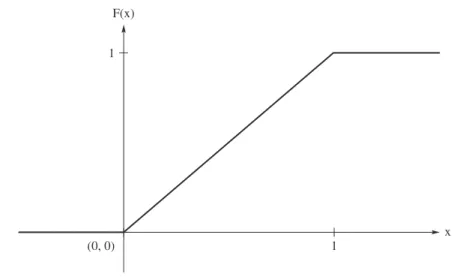
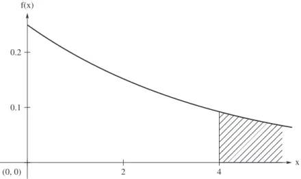
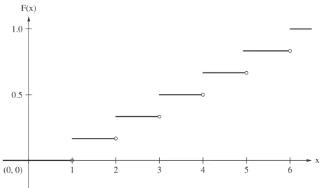
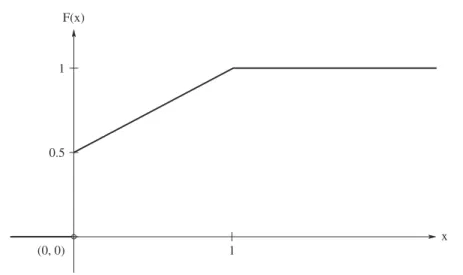
A mode of the distribution of a random variable X is a value of x that maximizes the pdf or pmf. For each of the following cdfsF(x), find pdff(x) [pmf in part(d)], the 25th percentile, and the 60th percentile.
Expectation of a Random Variable
This means, in general, the expected value of an output is not equal to the product of the expected values. Let the random variable X be the number of chips, out of two to be selected, that are marked $1.
Some Special Expectations
Find the mean and variance, if any, of each of the following distributions. Let a random variable X of continuous type have a pdf f(x) whose graph is symmetric with respect to tox=c. Show that the moment generating function of a random variable X having pdf f(x) =13, −1< x <2 is zero elsewhere.
If is a positive integer, show that R(m)(0) is equal to the moment of the distribution about the point b.
Important Inequalities
Since the numerator of the right-hand member of the previous inequality is σ2, the inequality can be written. In the following example, this upper bound and the exact probability value are compared in individual cases. In each of the cases in Example 1.10.1, the probability P(|X−µ| ≥kσ) and its upper bound 1/k2 differ significantly.
Because the last term on the right-hand side of the above equation is non-negative, we have
Distributions of Two Random Variables
Expectation
Note that the proof we gave of this theorem involves the discrete case, and Exercise 2.1.11 shows its extension to the vector case. The existence of the expected value of k1Y1+k2Y2 follows directly from the inequality and linearity of the triangle of integrals;. As in the univariate case, if it exists, the mgf of a random vector uniquely determines the distribution of the random vector.
These moment generating functions are, of course, marginal probability density functions.
Transformations: Bivariate Random Variables
Accordingly, the marginal pdf fY1(y1) of Y1 can be obtained from the joint pdf fY1,Y2(y1, y2) in the usual way by integrating over y2. We provide two illustrations that demonstrate the power of this technique by revisiting Examples 2.2.1 and 2.2.4. Here X1 and X2 have a common pmf. where µ1 and µ2 are fixed positive real numbers. Therefore pmf must be Y due to the uniqueness of mgfs. which is the same pmf as obtained in Example 2.2.1. Here X1 and X2 have a common pdf.
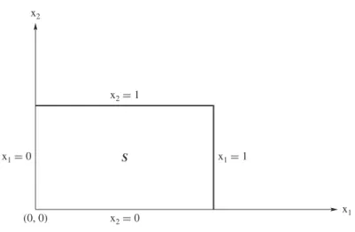
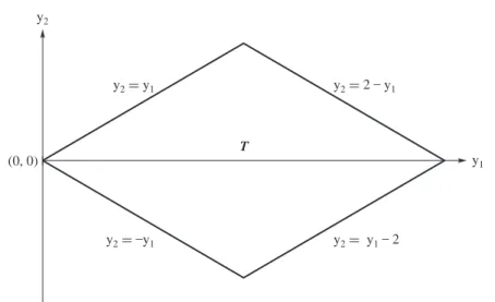
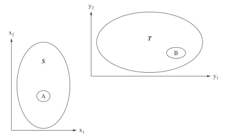
Hint: Use the inequalities 0< y1y2 < y2 <1 in considering the mapping fromS ontoT. Suppose X1 and X2 have the joint pdf. a) Show that the pdf of W is
Conditional Distributions and Expectations
It is called the conditional pdf of the continuous type of the random variable X2, given that the continuous type of the random variable X1 has the value x1. When fX2(x2)>0, the conditional pdf of the continuous random variableX1, given that the continuous type of the random variableX2 has the value x2, is defined by. If we did not know µ2, we could use one of two random variables to guess the unknown µ2.
Determine the conditional mean and variance of X2 if X1=x1, for x1= 1 or 2. Let X1 and X2 be two random variables such that there are conditional distributions and means. a) Calculate the marginal pdf of X and the conditional pdf of Y given X = x.
The Correlation Coefficient
For certain kinds of distributions of two random variables, say X and Y, the correlation coefficient ρ turns out to be a very useful property of the distribution. If ρ= 0, the variance of each conditional distribution of Y, given X =x, is σ22, the variance of the marginal distribution of Y. It is quite clear that the results of equations (2.4.7) hold if X and Y are random variables of the discrete type.
The correlation coefficients can therefore be calculated using the mgf of the joint distribution if that function is readily available.
Independent Random Variables
Conversely, condition (2.5.2) implies that the total cdf of (X1, X2) factors into the product of the marginal cdfs, which then implies, by Theorem 2.5.2, that X1 and X2 are independent. Thus, the independence of X1 and X2 means that the mgf of the joint distribution factors into the product of the functions that generate the moments of the two marginal distributions. The uniqueness of mgf means that the two probability distributions described by f1(x1)f2(x2) and f(x1, x2) are the same.
With random variables of the discrete type, the proof is made using summation instead of integration.
Extension to Several Random Variables
As in the bivariate case, the expected value of the random variable exists if it is then a complex integral. All previous definitions can be directly generalized to the case of n variables as follows. As in the one-variable and two-variable cases, this mgf is unique and uniquely determines the joint distribution of the n variables (and thus all marginal distributions).
E(Xn))′, that is, the expectation of a random vector is just the vector of the expectations of its components.
Transformations for Several Random Variables
The appropriate notational changes in Section 2.2 (to denote n-space as opposed to 2-space) are all that are needed to show that the joint pdf of the random variables Y1 = u1(X1, X2,. Considering the probability of the union of k mutually exclusive events and applying the change of variable technique to the probability of each of these events, it can be seen that the joint pdf of Y1 =u1(X1, X2,. It is easy to see that the absolute the value of each of the four Jacobians is equal to 1/42.
Y1 and Y2 are thus independent random variables according to theorem 2.5.1. Xn) is a function of the random variables, then mgf ofY is given by
Linear Combinations of Random Variables
Xn are independent and identically distributed (iid), we often say that these random variables constitute a random sample of size n from the joint distribution. Let X1 and X2 be two independent random variables such that the variances of X1 and X2 are respectively σ12 = k and σ22 = 2. Assuming that the three random variables involved are independent and uniformly distributed, calculate the mean and variance of the amount to be received.
Find the variance of the sum of 10 random variables if each variable has variance 5 and if each pair has a correlation coefficient 0.5.
The Binomial and Related Distributions
Then, by the rule of multiplication of probabilities, P(Y =y) =g(y) is equal to the product of the probabilities. Let be the number of successes of independent repetitions of a random experiment with probability of success= 23. Let be the number of successes during all independent repetitions of a random experiment with probability of success p= 14.
Show that the moment generating function of the negative binomial distribution is M(t) = pr[1−(1−p)et]−r.
The Poisson Distribution
Thus, the probability g(0, w+h) of zero changes in the interval of length w+his, according to postulate 3, is equal to the product of the probability g(0, w) of zero changes in the interval of length w and the probability [1−λh−o(h) ] of zero changes in a non-overlapping interval of length h. On the other hand, if X has a Poisson distribution with parameter m = µ, then the R command dpois(k,m) returns the value P(X = k). Xn are independent random variables and assume that Xi has a Poisson distribution with parameter mi.
By the last theorem, because the collaterals are independent of each other, Y has a Poisson distribution with parameter3.
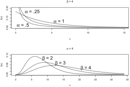
Let us now consider a special case of the gamma distribution in which α=r/2, where r is a positive integer and β = 2. For no apparent reason, we call the parameter the number of degrees of freedom of the distribution chi-square (or chi-square pdf). Find the uniform continuous distribution on the interval (b, c) that has the same mean and the same variance as a chi-square distribution with 8 degrees of freedom.
Show that the graph of the β pdf is symmetric about the vertical line through x= 12 ifα=β.
The Normal Distribution
Contaminated Normals
Suppose we observe a random variable that follows a standard normal distribution most of the time, but sometimes follows a normal distribution with a larger variance. Let Y have rounded distribution with pdfg(y) =φ(y)/[Φ(b)−Φ(a)], for a < y < b, zero elsewhere, whereφ(x) and Φ(x) are respectively the pdf and distribution function of a standard normal distribution. If a computer is available, examine the probabilities of an "outlier" for a contaminated normal random variable and a normal random variable.
Assuming a computer is available, plot the PDFs of the random variables defined in parts (a)–(d) of the last exercise.
The Multivariate Normal Distribution
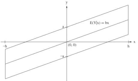
Although the mean of the conditional distribution of Y, given X =x, depends onx(unlessρ= 0), the varianceσ22(1−ρ2) is the same for all real values ofx. In this sense, most of the probability for the distribution of X and Y lies in the band. We say the total variation, (TV), of a random vector is the sum of the variances of its components.
Assuming a bivariate normal distribution, what is the best guess for the height of a woman whose husband is 6 feet tall.
The t-distribution