Wireless Networks

In the second part, a new RT-based scheduling system within the evolving cloud radio access network (C-RAN) architecture is proposed. My sincere gratitude goes to my sister Yasmin for always being my strong support and for the immense love she has given me throughout my life.

Introduction

Background and Motivation

The LTE/LTE-A system [5, 9] is the last introduced stage of the advanced series of telecommunication systems. The PHY layer information comprises the strength of the received signal, which fluctuates randomly due to noise and fading caused by the wireless channel.

State-of-the-Art and Thesis Outline

In Chapter 4, a fairly comprehensive study is introduced for the application of the RT model in the design of QoS-aware energy-efficient predictive scheduler in the LTE networks. After presenting these jitter models, the study showed a new trade-off between user equipment (UE) energy efficiency (EE) optimization and delay jitter performance for VoIP traffic services over LTE networks (ie, recently portrayed as VoLTE).

Contributions of the Thesis

Contributions of Chapter 2

A multi-objective optimization problem for EE UE and delay jitter subject to delay constraints for VoLTE services is formulated. The obtained results showed a new compromise between UE EE and packet delay jitter.

Introduction

The ray tracing (RT) propagation model is a deterministic approach which provides accurate modeling for predicting propagation effects in wireless communication channels based on information provided by a geographic information systems (GIS) database. . In Section 2.4, some of the reported ray tracing acceleration techniques used to improve the computational efficiency (in terms of processing time and energy consumption) of the ray tracing algorithm will be discussed.

Applications, Motivation and Recent Trends

The rest of this chapter is organized as follows: Section 2.2 presents some possible applications in which the ray tracing model is of particular interest, in addition to the motivation and recent trends in the technique. This chapter provides insight into how to implement a complete ray tracing solution using MATLAB.

Ray Tracing Algorithms

Shooting and Bouncing Rays Method
Image Method
Electric Field Evaluation

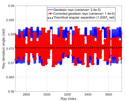
This technique, namely distributed wavefronts, assigns a weighting factor to each of the rays in the vicinity of the receiver. In the case of SBR, the accuracy is dependent on the angular separation of the launched beams.

Figure 2.1: Three-dimensional scene rendered using real-time FPGA ray tracer [2]

Ray Tracing Acceleration Techniques

Binary Space Partitioning
Space Volumetric Partitioning
Angular Z-Buffer

Facets in both half-spaces are labeled with respect to the facet surface normal vector. Therefore, the number of shading tests performed will be much less than the total number of facets that existed in the environment.

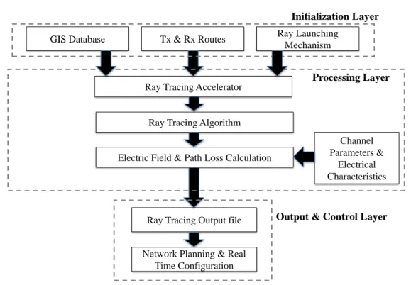
Ray Tracing Engine Architecture

Aspects within the anxel containing the traced ray are then arranged according to their distance from the origin of the ray. For a given observation point, the raypath will be sequentially tested for shading only with the listed facets located in the annex that spans the ray.

Figure 2.7: Ray tracing system architecture

MATLAB Ray Tracer

The developed architecture and its operation can be easily described with the help of the flowchart illustrated in Figure. After the initialization of the ray tracing parameters, the SVP partitioning algorithm takes place to register each facet completely or partially in a voxel, as explained in section 2.4.2.

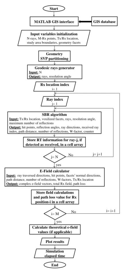
Figure 2.8: Flow chart describing the MATLAB implementation of the ray tracer

MATLAB GIS interface

Numerical Simulations and Verification with Commercial SoftwareCommercial Software

Line-of-Sight Test with Fixed Receiver Distance
Free Space Path Loss Test
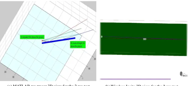
Two Ray Model Test
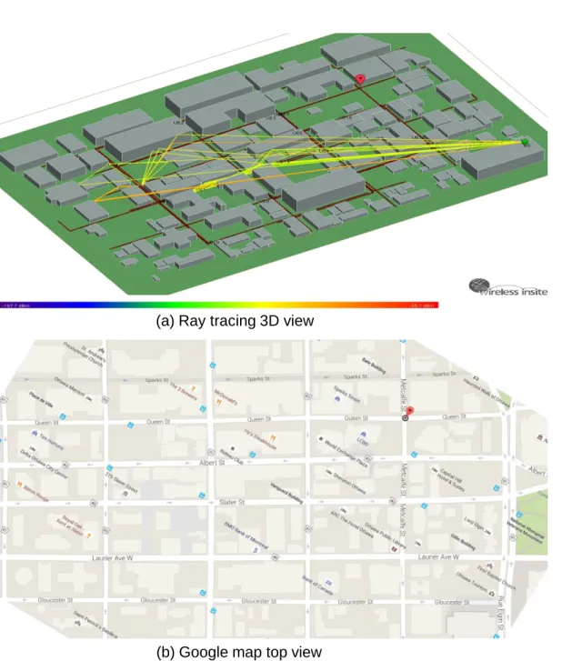
Urban Scenario Propagation Test

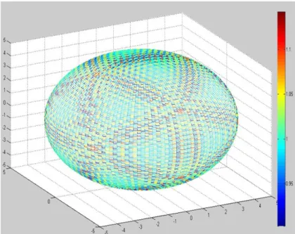
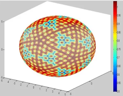
As a result, a uniform spatial distribution of all points on the surface of the sphere is obtained. A three-dimensional view of the test setup used for both the MATLAB and Insite environments is shown in Fig.

Figure 2.10: Snap shot for a sample of geodesic rays vs. corrected rays deviation angle The calculation of the angular separation between rays shows that the geodesic ray launching method does not provide ideal uniform distribution to the rays as explained

Chapter Summary

Introduction

However, more information about the future of the channel could be gained by tracking mobile radio trails in known environments. Section 3.4 shows the difference between the conventional channel-aware scheduler and the proposed scheduler.

Link Adaptation Analysis

Tlim→∞ Pout(T|γo) = P(γo) (3.4) The result of (3.4) represents the probability that the instantaneous SNR falls below the specified value γobtained at the beginning of the matching block when T >> τcoh. Isent(T|γo) = log2(1 +γo)T (3.7), whereas the effective amount of information reliably transmitted is:. 3.6) and (3.11) give us closed-form expressions for the variation of the outcome probability and the average reliable transmission rate, respectively, with respect to the adaptation horizon T.

Ray Tracing Based Prediction

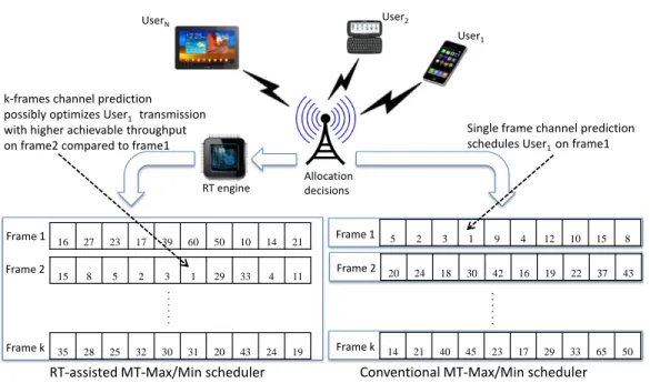
Therefore, the scheduler can obtain the future channel information provided by the RT mechanism for each user to be efficiently assigned to their optimal time slots and frequencies. Based on the widely used assumption in the literature [65] of block channel fading within a single 10 ms radio frame, the RT prediction is error-free for an error of up to 0.138 m in the device location.

Channel-Aware Scheduling

Conventional Channel-Aware Scheduler
The Proposed Optimal RT-Assisted Scheduler
Heuristic RT-Assisted Scheduler

However, solving (3.12) in the case of an RT-based scheduler is more complicated, since the scheduler must simultaneously handle k-frames at each step within a transmission cycle. The most complex sorting operation is performed at the beginning of each new transmission cycle (line 7), where N users are sorted on frames and is equal to O(kNlog(N)) (ie, ReqBuf f er is full of all users ).

Figure 3.2: Proposed RT-assisted vs conventional MT-Max/Min scheduler

Numerical Results

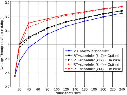
However, when N= 20, k= 4 RT scheduler does not improve the system's throughput performance compared to tok= 2 scheduler, due to the fact that the scheduler will benefit from knowing only the first and second frames of the channel , net ask= 2. This is due to the fact that the first BIP problem is the most complex problem solved by the optimal RT-based scheduler.

Figure 3.3: Throughput performance comparison

Chapter Summary

It is worth noting that the ability of our proposed schedulers to improve system throughput is highly dependent on how fast the channel changes in time (i.e., coherence time) and the chosen value of Using a faster fading channel model than the one used in our simulations and using large values is therefore expected to very positively affect the results of Fig.

Introduction

Related Work
Scope and Contribution

[74] showed that optimizing UE energy consumption inherently requires optimization of the base station (BS) downlink transmit power. In this work, we further expand the solution space of the scheduling problem for optimizing the UEs.

Figure 4.1: Energy efficiency for downlink predictive scheduling

System Description

System Model
UE Circuit Power Consumption
Channel Model

That rate is calculated based on the effective bandwidth theory (i.e. the double concept of effective capacity [75]) and will simultaneously meet all the user's individual connection requirements. This is supported by the assumption that the eNB (i.e. the transmitter in our analysis) is operating at the maximum allowed transmission power.

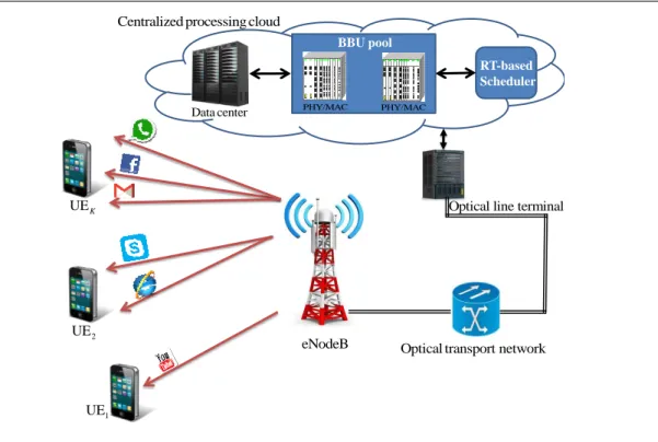
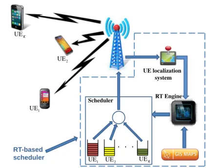
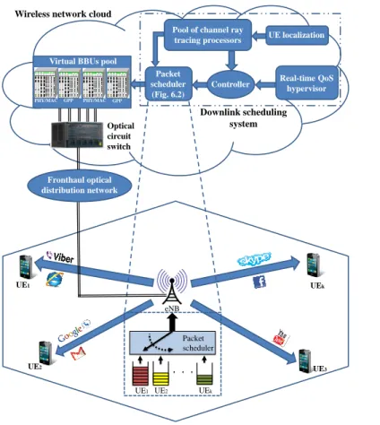
Proposed Predictive Scheduling System

The function of the localization system is to interactively determine the geographic location of each EU within the cell's coverage GIS map. Thus, the RT engine that predicts the CSI for each UE is part of the shared architecture explained in Fig.

Figure 4.4: Ray tracing based downlink scheduler system

Optimal Scheduler

General Formulation
Penalty Method-Based Formulation
Practical ON-OFF Formulation

In (4.10a), it is obvious that the penalty function added to the constrained problem presented in (4.9) is the full term added to Etot. It should also be noted from (4.10d) that the decision variable Ωk is permanently set to 1 to force its expression—which is similar to the total number of bits waiting to be transmitted for each user—to always appear in the cost function v ( 4.10a).

Heuristic Scheduler

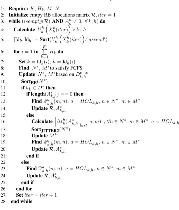
Heuristic Algorithm
Complexity Evaluation

FirstPr(i.e. in (4.5)), each TTI for each user is calculated using a reference channel model (i.e. discussed in detail in the next section). It is clear that the length of each user queue continuously changes over time, based on the number of allocated resources and their respective capacities during each scheduling period.

Figure 4.5: Heuristic algorithm flowchart for the proposed scheduler

Numerical Results

Scenario 1: QSBR Channel
Scenario 2: RT-based Channel

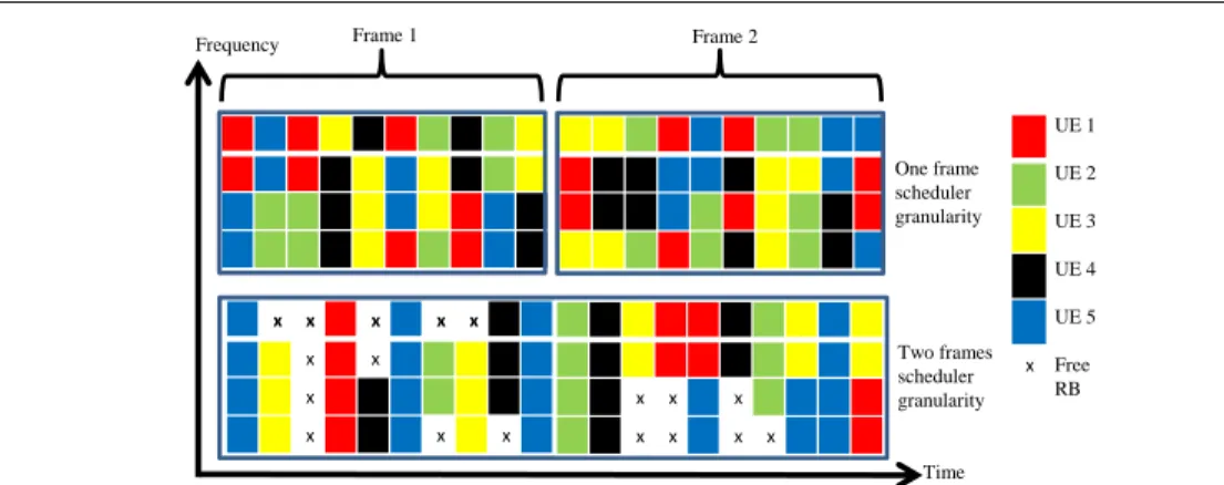
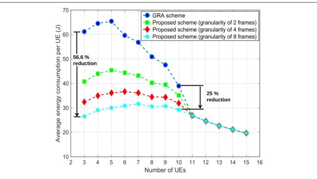
However, that effect is less pronounced in the case of the proposed scheme as the scheduling granularity increases compared to the GRA scheme. 4.12, both the buffers' stability performance and the system's admittance capacity for the proposed scheme showed a slight improvement over the GRA scheme as demonstrated in Fig.

Figure 4.6: 3D ray tracing experiment for part of Ottawa city

Chapter Summary

Thus, although we fail to increase the capacity of the system, our proposed scheme is still able to improve the EE of the UE by increasing the time granularity of the scheduler in the presence of slowly varying channels. On the other hand, despite having no effect on the scheduler's access capacity, in the presence of the slow fading channel the proposed scheme was able to improve the EE of the EU by up to 56.6% compared to the GRA -scheme.

Figure 4.19: Average energy consumption per UE ing the well known, site-specific, ray tracing approach.

Introduction

The rest of this chapter is organized as follows: In Section 5.2, a detailed analytical modeling of delay excitation in various queuing systems is presented. The optimization for VoLTE traffic delay harassment and its effect on the UE's EE in LTE multi-user environment is presented next in Section 5.3.

Analytical Approximation of Packet Delay Jitter in Simple QueuesSimple Queues

Background
Jitter modelling framework
Underutilized queue
Heavy loaded queue
Bridging case
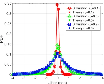
Numerical Simulations
Background
System Model and Problem Formulation
Heuristic Algorithms
Numerical Simulations

Equalization of service time in each channel state (decrease τJ) by channel inversion [97]. On the other hand, increasing the packet service time correlation sharpens the delay jitter distribution around zero (i.e., the delta term in Equation (5.12)).

Figure 5.1: Packet delay jitter evaluation for the M/M/1 queue

Chapter Summary

Introduction

Research Problem
Related Work
Scope and Contribution

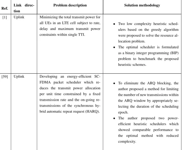
Despite having a similar definition, the application of the MA mode for the UE's EE enhancement in the uplink is different from that in the downlink. A summary of works that have considered UE EE in the downlink is given in Table 6.1.

Table 6.1: Some of the recent EE schedulers reported in literature

System Model

Utility-Based Scheduling
Energy-Efficient Scheduling

The above metric functions provide a quantitative measure of the QoS perceived by the corresponding UE traffic link. Energy-efficient operation for a UE in the downlink, as originally defined in [79], dictates the optimization of the operating time for the UE's receiver circuits subject to a packet delay constraint.

Delay Jitter Background

Moreover, relatively recent works [94, 128] have also addressed the problem of delay jitter within heterogeneous traffic environments. It can be noted that the studies highlighted above have mainly addressed the delay jitter problem at the network layer.

Problem Formulation

The constraint in (6.10b) sets a strict requirement for the scheduling of all packets waiting in the different queues of all UEs. The relaxation implies partial satisfaction of the constraint in (6.10b) for each UE connection based on a certain weighting mechanism.

Heuristic Solutions

SRV-Based Schedulers
PRV-Based Schedulers

Similar inspection for the complexity of the SRV-PO algorithm, in Table 6.3, leads to O(N M)+O(N M log(N M)). The main structure is similar to that of the SRV-based algorithms except for the sliding window loop in line 3.

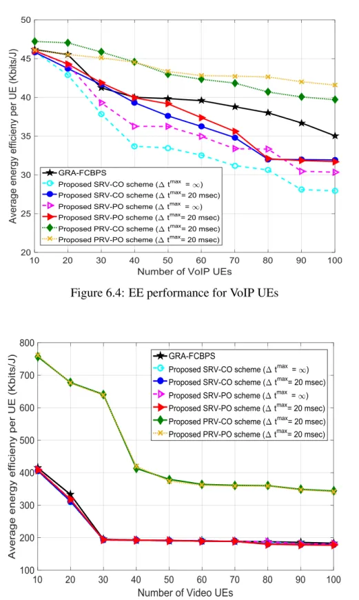
Table 6.3: SRV-PO algorithm 1: Require: K, H k , M , N

Numerical Results

The third conclusion is regarding the relative EE performance of the proposed SRV-CO and SRV-PO schedulers compared to the GRA-FCBPS. From another perspective, the SRV-PO scheme generally shows better performance (i.e., EE/delay-jitter trade-off) compared to the SRV-CO.