Accepted Manuscript

Accepted Manuscript

Deep convolutional neural networks for mobile capture device-based crop dis- ease classification in the wild

Artzai Picon, Aitor Alvarez-Gila, Maximiliam Seitz, Amaia Ortiz-Barredo, Jone Echazarra, Alexander Johannes

PII: S0168-1699(17)31261-9

DOI:

Reference: COMPAG 4242

To appear in:

Received Date: 15 October 2017

Revised Date: 5 March 2018 Accepted Date: 1 April 2018

Please cite this article as: Picon, A., Alvarez-Gila, A., Seitz, M., Ortiz-Barredo, A., Echazarra, J., Johannes, A., Deep convolutional neural networks for mobile capture device-based crop disease classification in the wild,

This is a PDF file of an unedited manuscript that has been accepted for publication. As a service to our customers

we are providing this early version of the manuscript. The manuscript will undergo copyediting, typesetting, and

review of the resulting proof before it is published in its final form. Please note that during the production process

errors may be discovered which could affect the content, and all legal disclaimers that apply to the journal pertain.

Deep convolutional neural networks for mobile capture

device-based crop disease classification in the wild.

Artzai Picon^a, Aitor Alvarez-Gila^a, Maximiliam Seitz^c,d, Amaia Ortiz-Barredo^a, Jone Echazarra^a, Alexander Johannes^d,∗

aComputer Vision, TECNALIA, Parque Tecnolgico de Bizkaia, C/ Geldo. Edificio 700, E-48160 Derio - Bizkaia (Spain)

bNEIKER, Plant health Dp, Arkaute Agrifood Campus, E-01080 Vitoria-Gasteiz, Araba (Spain)

cInstitute of Process Engineering in Plant Production, University of Hohenheim, 70599 Stuttgart

dBASF SE, Speyererstrasse 2, 67117 Limburgerhof (Germany)

Abstract

Fungal infection represents up to 50% of yield losses, making it necessary to ap- ply effective and cost efficient fungicide treatments, whose efficacy depends on infestation type, situation and time. In these cases, a correct and early identifi- cation of the specific infection is mandatory to minimize yield losses and increase the efficacy and efficiency of the treatments. Over the last years, a number of image analysis-based methodologies have been proposed for automatic image disease identification. Among these methods, the use of Deep Convolutional Neural Networks (CNNs) has proven tremendously successful for different vi- sual classification tasks.

In this work we extend previous work by Johannes et al. (2017) with an adapted Deep Residual Neural Network-based algorithm to deal with the de- tection of multiple plant diseases in real acquisition conditions where different adaptions for early disease detection have been proposed. This work analyses the performance of early identification of three relevant European endemic wheat diseases: Septoria (Septoria triciti), Tan Spot (Drechslera triciti-repentis) and Rust (Puccinia striiformis & Puccinia recondita). The analysis was done using

∗Corresponding author

Email address: [email protected](Alexander Johannes)

different mobile devices, and more than 8178 images were captured in two pi- lot sites in Spain and Germany during 2014, 2015 and 2016. Obtained results reveal an overall improvement of the balanced accuracy from 0.78 (Johannes et al. (2017)) up to 0.87 under exhaustive testing, and balanced accuracies greater than 0.96 on a pilot test performed in Germany.

Keywords: convolutional neural network, deep learning, image processing, plant disease, early pest, disease identification, Precision Agriculture, phytopathology

1. Introduction

Besides weeds, most relevant biotic stress factors in winter wheat production are caused by fungal pathogens. In cases of intensive production systems, like in Central Europe, these can cause yield losses up to 50% (Oerke (2006)). Hereby, an effective and cost efficient fungicide treatment adapted on the infestation

5

situation and time (Hanus (2008)) is compulsory. This requires continuous plant stock controls to monitor plant health, which are both time and cost intensive (K¨ubler (1994)). A key factor for an appropriate decision making in crop protection is the detailed knowledge of the occurrence of current pathogen species. The visual identification of fungal disease symptoms even at early

10

infestation stages and the correct assignment to a special pathogen is still a very challenging task due to similar stress symptoms caused byvarious pathogens and abiotic stress symptoms likewise(Oerke et al. (2010), Stafford (2000)). In view of vast agricultural regions where contact to crop protection experts is very limited, it would be a real advantage to provide easily accessible identification support

15

tools to enable effective infestation situation-based crop protection measures (Singh and Misra (2017)). In more advanced countries with well-trained farmers and good advisory structures, where normally very intensive production systems are established, there is the need to hold crop protection measures efficient, due to a constant increasing disease pressure. Here, an early pathogen detection

20

is the basic prerequisite to derivate the most effective crop protection measure

(Martinelli et al. (2015)). This demand gets underlined by the more frequent occurrence of resistant fungi races, which negatively affected the performance of modern fungicides (Brent and Hollomon (1995)).

In the last decades, significant efforts and various concepts in crop science

25

can be observed to ease plant health control by using sensor techniques and simulation models. In this context, thermography, chlorophyll fluorescence and hyperspectral sensors are seen as very promising technologies. Furthermore, it is stated that imaging systems are preferable to non-imaging systems for the purpose of detecting plant diseases Mahlein et al. (2012)). Nevertheless, the dis-

30

tribution of these technologies for decision support in broad agricultural practice is fairly low. Early studies around the year 2000 point out that the reason for the low usage are primarily the high uncertainty upon which the automatically gen- erated identification or prediction results are founded, and the excesively high complexity of the systems (Kuhlmann and Brodersen (2001),McCown (2002)).

35

In a more recent study, the missing of comprehensive techniques for rapid dis- ease detection is still underlined on the example of Fusarium spec. detection (Bauriegel and Herppich (2014)). With regard to developing countries, for sure it can be stated that the maturity of described technologies, will be much too expensive.

40

A recent approach to identify multiple plant diseases is using statistical infer- ence methods to setup picture recognition algorithms. These can be applied by using mobile capture devices, which allows a broad availability for agricultural practice (Johannes et al. (2017)). Within this work it was shown that there is a potential to improve the developed algorithm’s performance on the generation

45

of reliable early disease diagnosis. Deep Convolutional Neural Networks (CNNs) are seen as breakthrough for image classification and seem to be very promising for this purpose.

2. Related work

Classical Computational visual approaches have been extensively used to

50

address automated plant identification. In this sense, pioneering studies from Sannakki et al. (2011) automatically graded diseases present on plant leaves.

Their proposed algorithm employed image processing techniques to analyze the color-specific information on infected plants. A first k-means based clustering was performed for each image pixel to isolate the infected spots and subse-

55

quent grading was performed based on fuzzy logic techniques. Other works like Xie et al. (2016) focused on reducing the computational complexity of the automation algorithm with relative success. In 2016, Siricharoen et al. (2016) developed a technique that combined texture, color and shape to detect the presence of a specific disease on a plant. From 2014 to 2016, Johannes et al.

60

(2017) generated an extensive field database for wheat crop that included Septo- ria (Septoria triciti), Tan Spot (Drechslera triciti-repentis) and Rust (Puccinia striiformis, Puccinia recondita) diseases at different phenological stages over more than 36 wheat plant varieties. The algorithm was validated on real field conditions showing an AuC (Area under the Receiver Operating Characteristic

65

-ROC- Curve) above 0.80 and accuracies around 0.82 for late and medium stage diseases and around 0.76 for early stage diseases. The algorithm was based on a classical machine learning-supported image analysis approach, consisting of a first image preprocessing and normalization stage that included a preliminary filter to detect the candidate regions, and a second stage in which textural and

70

color descriptors from the candidates were coupled with a random forest based classifier. Although results were highly promising, the limited expressive power of the color and textural descriptors kept the model from further generalizing, thus laying on the bias extreme of the bias-variance trade-off. This means that the developed algorithm could not take advantage of a larger number of training

75

pictures.

As an alternative that has proven itself tremendously successful in overcom- ing the expressive power limitation that characterizes traditional workflow-based

computer vision approaches, Deep Convolutional Neural Networks (CNNs) pro- vide a flexible framework that allows for the definition of models that act both

80

as descriptive hierarchical feature extractor and as classifier. CNN network topologies can be extended (e.g. by stacking more convolutional layers) in such a way that their complexity grow to match the expressive power required by any given objective task and data availability. The best known example of this was 2012 ImageNet Large Scale Visual Recognition Competition (ILSVRC2012)

85

Russakovsky et al. (2015), won by almost 10 percent points by the CNN de- scribed in Krizhevsky et al. (2012a), which required the contenders to classify a set of images onto 1000 different classes after being trained on over a million images. The field of Computer Vision experienced a major shake-up that year, and ever since that event, deep learning-based solutions have consistently been

90

beating traditional workflow-based shallow approaches in almost every computer vision task -e.g. image classification, single object classification and object de- tection (Russakovsky et al. (2015)), semantic segmentation (Shelhamer et al.

(2016)), instance segmentation (Li and Malik (2016))), enabling the definition and addressing of new tasks that were not even possible up until the appear-

95

ance of these techniques (e.g. Visual Question Answering (Zhu et al. (2016)) or Dense Captioning (Johnson et al. (2016)), to name a few within the area of supervised learning- and even surpassing human performance at some of them (Russakovsky et al. (2015)).

All such approaches have been also extensively tested in a wide number of

100

applications, ranging from medical diagnosis in dermatological (Esteva et al.

(2017)) or histopathological images (Litjens et al. (2016); Arajo et al. (2017)), among others, to autonomous driving of cars ((Badrinarayanan et al. (2015) and drones (Gandhi et al. (2017))), or quality control in manufacturing industries (Masci et al. (2012)).

105

Agricultural applications are not an exception to this trend, and deep neural nets have been successfully been used to predict land use from remote sensing images (Hu et al. (2015)), plant phenotyping (Pound et al. (2016)) or weed scouting (Di Cicco et al. (2016)). As for plant disease identification, Sladojevic

et al. (2016) applied an AlexNet-like architecture (Krizhevsky et al. (2012a))

110

to model 13 different diseases from an image dataset obtained through inter- net online search. Initiatives such as PlantVillage (Hughes et al. (2015)) have allowed the generation of more than 50,000 expertly curated images of healthy and infected leaves of 14 different crops (apple, blueberry, corn, grape) and a total number of 26 different diseases. This database has served their promoters

115

to develop a disease identification classifier (Mohanty et al. (2016)) based on a pre-trained GoogleNet architecture (Szegedy et al. (2015)), where a transfer learning approach was followed to adequate the model to the plant disease iden- tification use case. Authors report an accuracy of 99.35% on their model on a held-out test set. However, when the algorithm is tested under conditions

120

different to the ones of the training database, the accuracy decreases down to as low as 31.4%. The fact that the database is taken under controlled conditions and the presence of only late stage diseases on the database precludes its use as a real digital farming application where early disease detection on uncontrolled illumination conditions is essential for a correct deployment. Besides that, these

125

algorithms do not consider the case where more than one disease are present in the same plant; therefore, models trained and tested on them will only be able to detect the most visible disease, which is not necessarily the one of most importance for the crop.

In this paper we extend the previous work on early disease detection from

130

Johannes et al. (2017) by presenting and validating in real field conditions a Convolutional Neural Network-based method that is able to cope both with early disease stages and simultaneous diseases.

3. Material & Methods

3.1. Training and validation dataset

135

An extensive dataset was generated to perform the training and validation of the proposed algorithm. For that, we extended the field database from Johannes et al. (2017), which contained a total number of 3637 images of wheat diseases

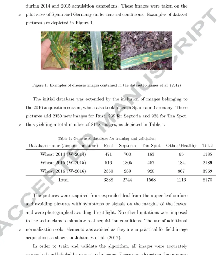
during 2014 and 2015 acquisition campaigns. These images were taken on the pilot sites of Spain and Germany under natural conditions. Examples of dataset

140

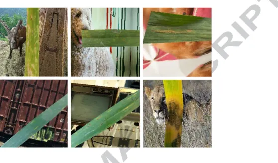
pictures are depicted in Figure 1.

Figure 1: Examples of diseases images contained in the datasetJohannes et al. (2017)

The initial database was extended by the inclusion of images belonging to the 2016 acquisition season, which also took place in Spain and Germany. These pictures add 2350 new images for Rust, 239 for Septoria and 928 for Tan Spot, thus yielding a total number of 8178 images, as depicted in Table 1.

145

Table 1: Generated database for training and validation

Database name (acquisition time) Rust Septoria Tan Spot Other/Healthy Total

Wheat 2014 (W-2014) 471 700 183 65 1385

Wheat 2015 (W-2015) 516 1805 457 184 2189

Wheat 2016 (W-2016) 2350 239 928 867 3969

Total 3338 2744 1568 1116 8178

The pictures were acquired from expanded leaf from the upper leaf surface and avoiding pictures with symptoms or signals on the margins of the leaves, and were photographed avoiding direct light. No other limitations were imposed to the technicians to simulate real acquisition conditions. The use of additional normalization color elements was avoided as they are unpractical for field image

150

acquisition as shown in Johannes et al. (2017).

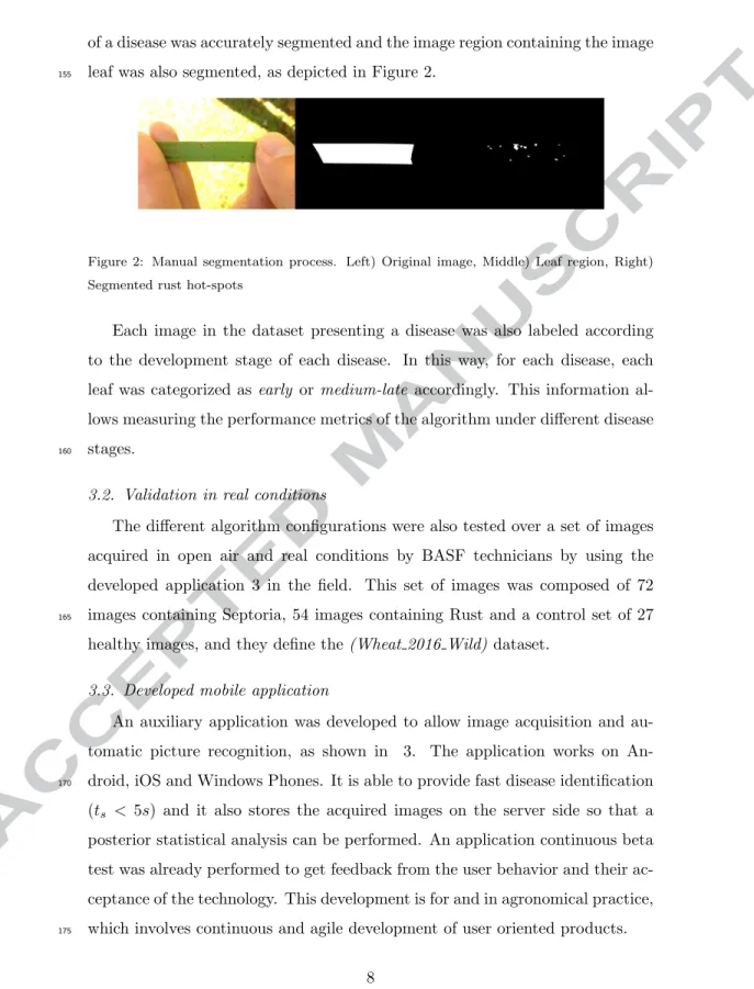
In order to train and validate the algorithm, all images were accurately segmented and labeled by expert technicians. Every spot depicting the presence

of a disease was accurately segmented and the image region containing the image leaf was also segmented, as depicted in Figure 2.

155

Figure 2: Manual segmentation process. Left) Original image, Middle) Leaf region, Right) Segmented rust hot-spots

Each image in the dataset presenting a disease was also labeled according to the development stage of each disease. In this way, for each disease, each leaf was categorized as early or medium-late accordingly. This information al- lows measuring the performance metrics of the algorithm under different disease stages.

160

3.2. Validation in real conditions

The different algorithm configurations were also tested over a set of images acquired in open air and real conditions by BASF technicians by using the developed application 3 in the field. This set of images was composed of 72 images containing Septoria, 54 images containing Rust and a control set of 27

165

healthy images, and they define the(Wheat 2016 Wild)dataset.

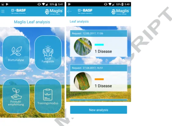
3.3. Developed mobile application

An auxiliary application was developed to allow image acquisition and au- tomatic picture recognition, as shown in 3. The application works on An- droid, iOS and Windows Phones. It is able to provide fast disease identification

170

(t_s < 5s) and it also stores the acquired images on the server side so that a posterior statistical analysis can be performed. An application continuous beta test was already performed to get feedback from the user behavior and their ac- ceptance of the technology. This development is for and in agronomical practice, which involves continuous and agile development of user oriented products.

175

Figure 3: Developed mobile application for disease identification

4. Adapting Deep Convolutional Neural Networks for Early-Stage Disease Detection

Common deep learning-based architectures for image classification have been designed and extensively tested to advantageously cope with tasks where clas- sification of an image involves the presence of an specific object on a significant

180

portion of the image (e.g. Deng et al. (2009)). Moreover, input images are nor- mally resized into the input size of the network (sizes typically not larger than 224 pixels) which, in the case of early disease identification, reduces the already small size of the incipient diseases, making these approaches not appropriate for the detection of subtle early symptoms.

185

Object detection approaches ( Uijlings et al. (2013), Girshick et al. (2014), Girshick (2015), Ren et al. (2015)) have successfully achieved good performance on object detection and they can be an appropriate alternative for the disease

identification problem. However, these networks are especially tailored to the typical object size of the dataset over which they are trained and are also nega-

190

tively affected by datasets where the object size present a large variance whose accuracy drops especially for small objects ( Herranz et al. (2016)). Moreover, Eggert et al. (2017) have recently demonstrated that the R-CNN topology has to be adapted to the targeted object size and that no single topology is able to cope with objects presenting a high size variance. The large variance of both

195

appearance and scale of each of the targeted diseases where the small scattered rust pustules compete with the big continuous clusters of Septoria precluded the use of an object detection approach.

Based on the previous considerations, we propose the adaption of a clas- sification deep neural network architecture family that has proven itself very

200

competitive: Deep Residual neural networks, presented in He et al. (2016a) and He et al. (2016b), which reformulated the transformation performed by regular convolutional network layers as learning a residual that gets added to an iden- tity mapping, thus allowing deeper architectures that ultimately enabled wining theILSVRC 2015 challenge classification task (Russakovsky et al. (2015)).

205

This work adapts the aforementioned network topology to deal with simul- taneous multiple disease detection, and to allow focusing on early diseases even on cases of very small relative coverage areas, and does so by including the enhancements detailed on the next paragraphs:

4.1. Image preprocessing and tile extraction

210

One of the main issues for early-stage disease detection on deep learning architectures is that common architectures downsample the input image into smaller images (e.g. 224×224 in the case of typical Resnets (He et al. (2016a))).

For general purpose image classification tasks, this approach maintains the se- mantic information present in the image while significantly reducing the number

215

of network parameters, thus reducing the number of required training images.

In cases where the early disease is characterized by small and subtle spots (such as inDrechslera triciti-repentisorSeptoria triciti), this approach can reduce or

even make the disease vanish from the image, making it impossible to detect.

To mitigate this effect, three different alternatives are tested to extract the tile

220

candidates that will feed the neural network.

4.1.1. Full image resize

As a baseline alternative, the high resolution image is resized into the net- work input size following common approaches for deep learning architectures such as Krizhevsky et al. (2012a); He et al. (2016a). In this approach, the whole

225

image is downsampled regardless of the size of the leaf within the image.

4.1.2. Leaf mask crop

In this approach, the image is cropped to the bounding rectangle that con- tains the leaf element on the image. The extent of the leaf element is provided by expert annotation at training stage and by the end user at test time, by using

230

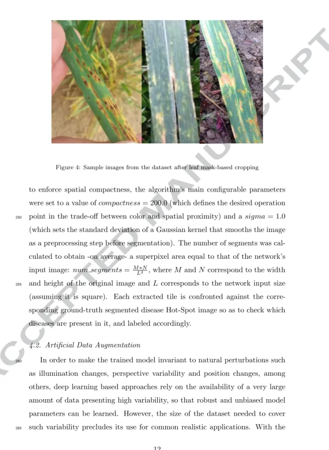
the leaf mask selection approach proposed in Johannes et al. (2017). Semantic segmentation of leaves has also been tested with good results, but it is out of the scope of this work. Intuitively, cropping the image into the leaf bounding rectangle diminishes the detail loss by discarding non-relevant areas of the orig- inal image before downsampling, specially for early-stage diseases. Details can

235

be appreciated in figure 4.

4.1.3. Superpixel based tile extraction

As an alternative, in order to avoid a significant downscaling of the por- tion of the image that might contain potential diseases (i.e. the leaf mask), which could degrade the visual features of the early-stage diseases, we propose

240

to segment the input image in a group of roughly homogeneous regions called superpixels. This segmentation pipeline relies on the Simple Linear Iterative Clustering (SLIC) superpixel extraction algorithm from Achanta et al. (2012).

SLIC adapts ak-means clustering-based approach in the CIELAB color space while keeping a configurable spatial coherence so as to enforce a certain com-

245

pactness. All superpixels not intersecting with the leaf mask are discarded, while the rest are independently resized to the neural network’s input size. In order

Figure 4: Sample images from the dataset after leaf mask-based cropping

to enforce spatial compactness, the algorithm’s main configurable parameters were set to a value ofcompactness= 200.0 (which defines the desired operation point in the trade-off between color and spatial proximity) and asigma= 1.0

250

(which sets the standard deviation of a Gaussian kernel that smooths the image as a preprocessing step before segmentation). The number of segments was cal- culated to obtain -on average- a superpixel area equal to that of the network’s input image: num segments= ^M∗N_L2 , whereM andN correspond to the width and height of the original image and L corresponds to the network input size

255

(assuming it is square). Each extracted tile is confronted against the corre- sponding ground-truth segmented disease Hot-Spot image so as to check which diseases are present in it, and labeled accordingly.

4.2. Artificial Data Augmentation

In order to make the trained model invariant to natural perturbations such

260

as illumination changes, perspective variability and position changes, among others, deep learning based approaches rely on the availability of a very large amount of data presenting high variability, so that robust and unbiased model parameters can be learned. However, the size of the dataset needed to cover such variability precludes its use for common realistic applications. With the

265

Figure 5: Superpixel boundaries extracted over images from the training dataset by applying

SLIC

aim of increasing the training set size and its variability, image augmentation techniques are frequently applied. Although recent models suggest that even realistic illumination color cast variations can be achieved through proper illu- minant estimation techniques (Galdran et al. (2017)), typically just basic ge- ometrical transformations are applied (Simonyan and Zisserman (2014)), such

270

as flipping, translations or rotations, but could include any other kind of affine and non-linear transformations, as long as the ground truth label does not get modified by the change (for the case of semantic segmentation-like annotations, these should also be transformed in parallel). At our algorithm’s training stage, each image is geometrically modified with a random transformation, which as-

275

sures better variability on the training images by acting as a regularizer. In order to avoid class imbalance during training (Japkowicz and Stephen (2002)), each class is also uniformly sampled from the dataset, thus yielding an equal percentage of each disease class during training.

Our preliminary studies showed that, although there was a high variety of

280

image backgrounds on the training dataset, the algorithm failed when elements with similar appearance to that of the disease appeared in the background of the image. In order to minimize this problem, a percentage of the image samples drawn during the training stage were sub-imposed with a random background image by previously extracting the portion of the image corresponding to the

285

leaf mask as depicted in 6. These random images were extracted from the Ima- genet ILSVRC15 dataset (Russakovsky et al. (2015)). This intuitively increases

background variability, helping the model to distinguish among a higher set of backgrounds.

Figure 6: Full resized images with the sub-imposed artificial background

4.3. Network topology

290

A Deep Residual Neural Network with 50 layers and 224×224 input image size was selected for our classification task, given the required trade-off between network capacity-complexity and training set size. The architecture is based on that presented in He et al. (2016a) asResnet-50. Our topology shares with He et al. (2016a) the inclusion of a batch normalization (Ioffe and Szegedy (2015))

295

and a Rectifier Linear Unit (ReLU) layer after each convolution operation. It also preserves the same combination of different kind of building blocks: a first type, namedidentity block, comprises two 1×1 convolutions with a 3×3 convolution in between and a direct skip connection bypassing input and output

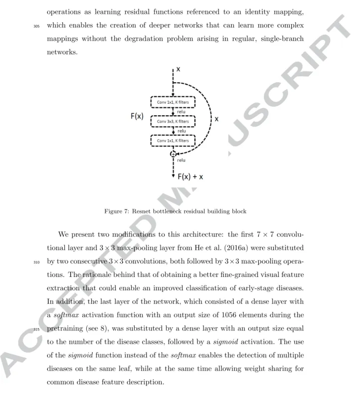
; meanwhile, a second kind named bottleneck residual building block adds a 1×1

300

convolution in the skip connection (converting it into aprojection shortcut) in order to enable a change in dimensions as depicted in 7. As described in He et al.

(2016a,b), the use of skip connections allows for a reformulation of convolutional

operations as learning residual functions referenced to an identity mapping, which enables the creation of deeper networks that can learn more complex

305

mappings without the degradation problem arising in regular, single-branch networks.

Figure 7: Resnet bottleneck residual building block

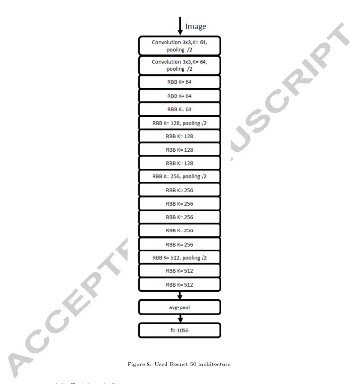
We present two modifications to this architecture: the first 7×7 convolu- tional layer and 3×3 max-pooling layer from He et al. (2016a) were substituted by two consecutive 3×3 convolutions, both followed by 3×3 max-pooling opera-

310

tions. The rationale behind that of obtaining a better fine-grained visual feature extraction that could enable an improved classification of early-stage diseases.

In addition, the last layer of the network, which consisted of a dense layer with a softmax activation function with an output size of 1056 elements during the pretraining (see 8), was substituted by a dense layer with an output size equal

315

to the number of the disease classes, followed by asigmoid activation. The use of thesigmoid function instead of thesoftmax enables the detection of multiple diseases on the same leaf, while at the same time allowing weight sharing for common disease feature description.

Figure 8: Used Resnet 50 architecture

4.4. Training pipeline

320

The training workflow comprises a three-stage learning process. In the first stage (pretraining), we extend the Imagenet dataset (Russakovsky et al. (2015))

by including images of additional plant species classes for a total of 1056 classes, and modify the original Resnet50 architecture accordingly, by substituting the output fully connected layer (originally with 1000 output units and a softmax

325

activation) by one with 1056 output units. This network is then trained from scratch (i.e. initialized with pseudo-random weights) until convergence on the task of 1056 class classification.

The second stage corresponds to a constrained fine-tuning one, in which we replace the aforementioned dense layer of 1056 outputs and softmax activation

330

by a dense layer of three output units (one per disease) and a sigmoid activation.

The predictive task is now the final one, i.e. that of predicting whether each of the diseases is present in the input image, and all the layers, except for the last dense one, are initialized with the weights learned in the first stage and are kept frozen. The last dense layer is randomly initialized, and it is the only one

335

allowed to modify its weights during learning.

The final training stage completes the fine-tuning by starting from the weights resulting from the previous stage and unfreezing all the layers, thus yielding a free, unconstrained training.

During the training stage, each image from the training dataset is prepro-

340

cessed by the tile extraction module by one of the three methods proposed in 4.1.

As a result, a tile (or group of tiles in case of the superpixel-based segmenta- tion) is obtained for each image and the label of each of the tiles is derived from the manually segmented images in the dataset. The process is shown in Fig- ure 9. The obtained tiles are drawn assuring equal distribution among all the

345

disease classes and the healthy plant class. In the case of The fully-convolutional network the obtained tiles

Each drawn tile is geometrically augmented by means of random linear ge- ometric distortions such as zoom, perspective, rotation and displacement, and the previously described artificial background is sub-imposed on a fraction of

350

them to increase background variability. The obtained image, paired with the class memberships, is used to train the convolutional neural network model.

The network was trained using Stochastic Gradient Descent (SGD) opti-

mization with an initial learning rate of 10⁻⁴, a learning rate decay of 10⁻⁶ and a momentum of 0.9. The weights of the last layer of the network were first

355

trained during 100 epochs while keeping the rest frozen, and afterwards the full network was trained.

CNN model train x

RGB Image

Ground-Truth Image

Superpixel based clustering

Tile cropping

Image

augmentation Artificial background

y

Figure 9: Training process pipeline. Each of the three independent flows refer to the one of the methods proposed in 4.1; from top to down:full image resize,leaf mask cropandsuperpixel based tile extraction

4.5. Fully Convolutional Network

Fully convolutional networks (FCN, Lin et al. (2013), Long et al. (2015))

360

have proven successful in reducing the potential overfitting that could arise from the use of fully connected layers in the last steps of traditional network architectures (Krizhevsky et al. (2012b), Simonyan and Zisserman (2014)), with the additional benefit of enabling inference over images of different sizes. The FCN approach substitutes such dense layers by convolutional layers with a 1×1

365

kernel, where the number of filters for the last layer equals the number of classes on the classification task. This allows for the generation of one feature map for each corresponding category on the task directly over the full-size image. For the analyzed classification task, this feature map is merged through a global average pooling layer. In this work we compare our proposed approaches against a fully

370

convolutional Resnet50 network, where the final convolutional layer substitutes the densely connected layer. A final global average pooling layer integrates the responses over the whole image. The proposed network has been trained both patch-wise and image-wise and tested on the fully sized image as proposed by Long et al. (2015).

375

5. Deployment Pipeline

The version of the algorithm deployed on-line is based on a roughly simi- lar but simplified version of the training pipeline. The leaf-mask is estimated by an estimation module from a rough input provided by the user using the method described in Johannes et al. (2017), which relies on Chan and Vese’s

380

active contours-based segmentation algorithm (Chan and Vese (2001)). The es- timated leaf-mask, together with the original RGB image, are used to feed the tile extraction module configured with one of the aforementioned alternatives (see 4.1). The extracted tiles are then passed to the augmentation module, which automatically generates a pre-configured number of augmented images to

385

be analyzed by the network model (trained as described in 4.4), with all of its outcomes being then averaged (see Figure 10). This augmentation and averaging process acts as a regularizer, by somehow mimicking the posterior probability distribution over some of the possible variations that a certain input image may present when being captured. The probability estimations from the different

390

tiles are integrated on a final classifier that takes the average probability from the tiles and returns a final decision and an associated confidence.

P(ci|y,tilei)

P(ci|y,tilej)

y Image augmentation

based sampling CNN model output

P(c_i|y) estimation from samples for

each tile

RGB Image Leaf Mask detection

Leaf level decision

Figure 10: Deployment framework. Left) RGB Image, Middle) Superpixel clustered image, Right) Leaf region tiles augmentation. The test-time augmentation yields a probability density function that is used to obtain a more robust classification estimate, as well as the associated confidence.

6. Results

The different configurations of the algorithm were first validated using the wheat dataset described in Section 3.1. This validation was then confirmed by

395

performing in-situ testing campaign in real field conditions (Section 3.2).

6.1. Validation set results

A training database was created with the images from theW−2014,W−2015 andW−2016 datasets defined in Table 1. In order to avoid bias, the dataset was divided into 80% of the images for training, another 10% for validation and a

400

final 10% for the testing set. The picture acquisition date was used as set division criterion, by not allowing pictures taken on the same day to be selected as part of different sets. The Area under the Receiver Operating Characteristic (ROC)

Curve (AuC) was selected as the most suitable algorithm performance metric, in order to account for the class imbalance present in the dataset (in such cases,

405

the use of accuracy is discouraged). The AuC for a binary classification problem is constructed by first sorting all the samples by the disease presence probability predicted by the model for each of them. The classification threshold value is then moved all the way from 0 to 1, and the result at each threshold value is mapped into the plot representing False Positive (x-axis) vs. True Positive rates

410

(y-axis), and measuring the resulting area (in the [0, 1] range, higher is better) under such curve as explained in Johannes et al. (2017). Computed values of sensitivity, specificity and balanced accuracy (BAC, as defined in eq. 1) for the different diseases are also provided for the threshold value that maximizes the validation set accuracy.

415

BAC= Sensitivity+Specif icity

2 (1)

Table 2 shows the obtained results. They clearly show that the use of the full image for identification performed worse than when using any of the proposed cropping techniques. Both superpixel-based cropping or leaf mask cropping in- creases the obtained AuC and balanced accuracy with respect to not cropping at all. Overall, the superpixel clustering approach works better for small spot

420

diseases, such as Tan Spot (Drechslera triciti-repentis) and Rust (Puccinia stri- iformis & Puccinia recondita), and a bit worse for largely spread diseases such as Septoria (Septoria triciti) . When using the artificial background augmenta- tion approach, the trained network’s AuC increases in all cases and are depicted in Figure 11. In the specific case of leaf-mask crop-based tile extraction, the use

425

of artificial background increases the network performance to supersede the one obtained with the superpixel approach.

6.1.1. Evaluation of Fully Convolutional Networks

The fully convolutional network described in Section 4.5 was trained both over the full-image and over randomly selected patches extracted from the full

430

image as proposed by Long et al. (2015), and the obtained models were applied

Table 2: Validation results with Resnet50 topology

Network Topology Tile extraction Artificial Background Disease AuC Sens Spec BAC

Resnet50 Full False Septoria 0.93 0.82 0.89 0.88

Resnet50 Full False Rust 0.94 0.91 0.89 0.90

Resnet50 Full False Tan Spot 0.82 0.68 0.84 0.76

Resnet50 Leafmask False Septoria 0.94 0.88 0.88 0.88

Resnet50 Leafmask False Rust 0.95 0.87 0.93 0.90

Resnet50 Leafmask False Tan Spot 0.90 0.79 0.87 0.83

Resnet50 Superpixel False Septoria 0.92 0.88 0.84 0.86

Resnet50 Superpixel False Rust 0.97 0.87 0.96 0.92

Resnet50 Superpixel False Tan Spot 0.86 0.80 0.80 0.80

Resnet50 Full True Septoria 0.93 0.91 0.80 0.86

Resnet50 Full True Rust 0.92 0.88 0.84 0.86

Resnet50 Full True Tan Spot 0.84 0.82 0.73 0.78

Resnet50 Leafmask True Septoria 0.94 0.87 0.89 0.88

Resnet50 Leafmask True Rust 0.96 0.92 0.90 0.91

Resnet50 Leafmask True Tan Spot 0.88 0.81 0.84 0.83

Resnet50 Superpixel True Septoria 0.92 0.88 0.88 0.88

Resnet50 Superpixel True Rust 0.97 0.87 0.96 0.93

Resnet50 Superpixel True Tan Spot 0.85 0.80 0.81 0.80

Figure 11: AuC results on superpixel and artificial background. Left)Tan Spot, Middle) Septoria, Right) Rust

to the full image. Results depicted in Table 3 show that the use of the full-sized images for training yields too low AuC values and that the use of a random crop- based approach for training provides better results. Both results are, however, far from the ones obtained by the other proposed methods.

435

6.1.2. Evaluation of online augmentation

We also measured the effect of the test-time augmentation averaging for the deployment pipeline described in Section 5 considering 1, 3, 5 and 7 aver- aged images. Our results (see Table 4) indicate that the online augmentation increases overall AuC by 2%.

440

Table 3: Validation results with Resnet50fc topology

Network Topology Tile extraction Artificial Background Disease AuC Sens Spec BAC

Resnet50fc image-wise True Septoria 0.58 0.75 0.39 0.57

Resnet50fc image-wise True Rust 0.69 0.56 0.74 0.65

Resnet50fc image-wise True Tan Spot 0.59 0.33 0.85 0.59

Resnet50fc patch-wise True Septoria 0.63 0.45 0.63 0.66

Resnet50fc patch-wise True Rust 0.83 0.72 0.86 0.79

Resnet50fc patch-wise True Tan Spot 0.75 0.56 0.81 0.69

Table 4: Performance improvement with online augmentation

Number of AuC AuC AuC AuC

augmented images Septoria Rust Tan Spot Average

1 0.94 0.96 0.88 0.92

3 0.95 0.97 0.89 0.94

5 0.95 0.97 0.89 0.94

7 0.95 0.96 0.89 0.93

6.1.3. Evaluation of early-stage disease classification

In order to quantify the performance of the algorithm on detecting early- stage diseases, the validation and test datasets were divided according to the degree of development of each disease. In this way, subsets corresponding to early and medium-late stages were created. AuC, sensitivity and specificity of

445

these datasets were also calculated so as to assess the influence of the disease evolution on the ability of the model to accurately predict its presence or ab- sence. Table 5 shows the results obtained for the early-stage disease detection scenario for the Resnet50 topology under the different considered configurations, while Table 6 does so for the medium-late state case.

450

Table 5: Validation results with Resnet50 topology in early diseases

Network Topology Tile extraction Artificial Background Disease AuC Sens Spec BAC

Resnet50 Full False Septoria 0.91 0.72 0.92 0.82

Resnet50 Full False Rust 0.88 0.61 0.93 0.77

Resnet50 Full False Tan Spot 0.82 0.64 0.85 0.75

Resnet50 Leafmask False Septoria 0.94 0.86 0.87 0.87

Resnet50 Leafmask False Rust 0.83 0.65 0.85 0.75

Resnet50 Leafmask False Tan Spot 0.75 0.74 0.69 0.71

Resnet50 Superpixel False Septoria 0.93 0.73 0.93 0.83

Resnet50 Superpixel False Rust 0.96 0.87 0.94 0.90

Resnet50 Superpixel False Tan Spot 0.83 0.72 0.80 0.76

Resnet50 Full True Septoria 0.94 0.83 0.91 0.87

Resnet50 Full True Rust 0.89 0.73 0.89 0.81

Resnet50 Full True Tan Spot 0.86 0.75 0.81 0.78

Resnet50 Leafmask True Septoria 0.96 0.93 0.92 0.92

Resnet50 Leafmask True Rust 0.93 0.81 0.91 0.86

Resnet50 Leafmask True Tan Spot 0.87 0.76 0.86 0.81

Resnet50 Superpixel True Septoria 0.94 0.87 0.90 0.88

Resnet50 Superpixel True Rust 0.96 0.87 0.93 0.90

Resnet50 Superpixel True Tan Spot 0.82 0.68 0.84 0.76

Table 6: Validation results with Resnet50 topology in medium-late diseases

Network Topology Tile extraction Artificial Background Disease AuC Sens Spec BAC

Resnet50 Full False Septoria 0.92 0.79 0.88 0.84

Resnet50 Full False Rust 0.89 0.77 0.95 0.86

Resnet50 Full False Tan Spot 0.82 0.65 0.87 0.76

Resnet50 Leafmask False Septoria 0.93 0.85 0.85 0.85

Resnet50 Leafmask False Rust 0.90 0.82 0.87 0.84

Resnet50 Leafmask False Tan Spot 0.72 0.69 0.68 0.69

Resnet50 Superpixel False Septoria 0.96 0.92 0.91 0.92

Resnet50 Superpixel False Rust 0.97 0.91 0.95 0.93

Resnet50 Superpixel False Tan Spot 0.85 0.74 0.83 0.78

Resnet50 Full True Septoria 0.94 0.86 0.87 0.87

Resnet50 Full True Rust 0.93 0.81 0.90 0.86

Resnet50 Full True Tan Spot 0.88 0.78 0.83 0.81

Resnet50 Leafmask True Septoria 0.95 0.89 0.89 0.89

Resnet50 Leafmask True Rust 0.96 0.87 0.92 0.90

Resnet50 Leafmask True Tan Spot 0.85 0.74 0.87 0.80

Resnet50 Superpixel True Septoria 0.96 0.90 0.90 0.90

Resnet50 Superpixel True Rust 0.97 0.91 0.94 0.93

Resnet50 Superpixel True Tan Spot 0.83 0.72 0.87 0.80

It can be appreciated that the use of a common deep learning approach does not improve the results obtained from Johannes et al. (2017), obtaining an average balanced accuracy (BAC) of 0.78. Both the superpixel approach and the leaf mask resize approach superseded the use of the full image. It can also be appreciated that the use of the leaf mask resizing approach does not improve

455

the performance obtained by the full image approach and it was necessary to include the artificial background based augmentation during training, resulting into higher performance values both in AuC and in balanced accuracy.

6.2. System testing under real conditions

The different algorithm configurations were then tested over a set of images

460

acquired in real conditions by BASF technicians by using the developed ap- plication (3). This set of images comprised 77 images containing Septoria, 54 images containing rust and a control set of 27 healthy images. Diseases were in advanced stage as pictures were acquired in late season. Values for specificity and sensitivity were calculated. The balanced accuracy (average sensitivity and

465

specificity) was averaged for the different diseases and provided as a final per- formance metric.

Table 7: Testing results on images taken under real field conditions

Network Topology Tile extraction Artificial Background Disease Sens Spec BAC

Resnet50 Full False Septoria 0.73 1.00 0.86

Resnet50 Full False Rust 0.94 0.98 0.96

Resnet50 Leafmask False Septoria 0.93 0.73 0.83

Resnet50 Leafmask False Rust 1.00 0.97 0.98

Resnet50 Superpixel False Septoria 0.98 0.78 0.88

Resnet50 Superpixel False Rust 0.98 0.98 0.98

Resnet50 Full True Septoria 0.73 1.00 0.87

Resnet50 Full True Rust 0.94 0.98 0.96

Resnet50 Leafmask True Septoria 0.80 0.98 0.89

Resnet50 Leafmask True Rust 1.00 0.92 0.96

Resnet50 Superpixel True Septoria 0.94 0.96 0.96

Resnet50 Superpixel True Rust 1.0 0.96 0.98

As it can be seen in Table 7, the obtained results are in consonance with the validation tests from 6.1. The use of the full image with a simple unmodified network produced lower balanced accuracy, specially forSeptoria triciti. This

470

can be also corroborated in other studies when applying the trained models to images not acquired under same conditions as the training dataset (Mohanty et al. (2016)). When applying the artificial background trained model over

the leaf mask crop approach, balanced accuracy values increase up to 0.96 for rust (Puccinia striiformis & Puccinia recondita) and 0.89 for Septoria triciti.

475

The superpixel-guided clustering-based technique combined with artificial back- ground training obtains the best results, with a balanced sensitivity of 0.98 for rust and a 0.96 for Septoria triciti. These results are significantly superior to those obtained by using classical computer vision techniques and reported in Jo- hannes et al. (2017), where balanced accuracies were 0.78 forSeptoria tricitiand

480

0.79 for rust.

6.3. Deployment

The algorithm was deployed under TensorFlow library as a scalable service into a Docker image with TCP communication capabilities that runs on server side with no GPU requirements. These services can be deployed in a distributed

485

way in order to balance load requirements. The average processing time of the algorithm was 0.9 (std= 0.43) seconds for the leaf mask resizing approach and 1.9 (std = 0.62) seconds for the superpixel-based approach. This algorithm is twice as fast as the speeds reported at Johannes et al. (2017).

7. Conclusions

490

In this work we presented new developments for the automatic multi-disease identification algorithm presented in Johannes et al. (2017) for field acquisition conditions. We enhanced the results from Johannes et al. (2017) by making use of a Residual Neural Network that included several improvements on the augmentation scheme and on the tile cropping. The use of these enhancements

495

support early disease detection while maintaining high specificities. The algo- rithm was validated over three different diseases: Septoria (Septoria triciti), Tan Spot (Drechslera triciti-repentis) and Rust (Puccinia striiformis & Puccinia re- condita) on wheat images, and it has been deployed on a real smart-phone application and validated under real field conditions as well.

500

Observed results on real conditions testing show that Balanced Accuracy values increased from 0.78 on the classical approach to an average BAC of

0.84 when using a Residual Neural Network without any further improvement.

However, this caused low specificities that could not assure high reliability on the detection in real case scenario, specially on early diseases, where the average

505

BAC was 0.78. The improvements on the confidence estimation, the super pixel segmentation approach and the artificial background training increased the performance of the algorithm up to an average Balanced Accuracy of 0.87 both for early and late diseases. The use of the online image augmentation increases these AuCs by an additional 2% We also proved, for the first time,

510

that a deep learning application can work with good performance on real natural conditions pilots for plant disease identification and cope with multiple diseases obtaining Balanced Accuracies greater than 0.96 in Germany.

As next steps, a large scale pilot is being held in Germany at the moment to further validate the obtained results. The proposed algorithm will also be

515

extended to different countries, diseases and crops to analyze the algorithm’s generalization power.

References

Achanta, R., Shaji, A., Smith, K., Lucchi, A., Fua, P., S¨usstrunk, S., 2012. Slic superpixels compared to state-of-the-art superpixel methods. IEEE transac-

520

tions on pattern analysis and machine intelligence 34, 2274–2282.

Arajo, T., Aresta, G., Castro, E., Rouco, J., Aguiar, P., Eloy, C., Polnia, A., Campilho, A., 2017. Classification of breast cancer his- tology images using Convolutional Neural Networks. PLOS ONE 12, e0177544. URL: http://journals.plos.org/plosone/article?id=10.

525

1371/journal.pone.0177544, doi:10.1371/journal.pone.0177544.

Badrinarayanan, V., Kendall, A., Cipolla, R., 2015. SegNet: A Deep Convolutional Encoder-Decoder Architecture for Image Segmentation.

arXiv:1511.00561 [cs] URL: http://arxiv.org/abs/1511.00561. arXiv:

1511.00561.

530

Bauriegel, E., Herppich, W.B., 2014. Hyperspectral and chlorophyll fluorescence imaging for early detection of plant diseases, with special reference to fusarium spec. infections on wheat. Agriculture 4, 32–57.

Brent, K.J., Hollomon, D.W., 1995. Fungicide resistance in crop pathogens:

How can it be managed? Citeseer.

535

Chan, T.F., Vese, L.A., 2001. Active contours without edges. IEEE Transactions on image processing 10, 266–277.

Deng, J., Dong, W., Socher, R., Li, L.J., Li, K., Fei-Fei, L., 2009. ImageNet:

A large-scale hierarchical image database, in: IEEE Conference on Computer Vision and Pattern Recognition, 2009. CVPR 2009, pp. 248–255. doi:10.

540

1109/CVPR.2009.5206848.

Di Cicco, M., Potena, C., Grisetti, G., Pretto, A., 2016. Automatic Model Based Dataset Generation for Fast and Accurate Crop and Weeds Detection. arXiv preprint arXiv:1612.03019 URL:https://arxiv.org/abs/1612.03019. bib- tex: di2016automatic.

545

Eggert, C., Brehm, S., Winschel, A., Zecha, D., Lienhart, R., 2017. A closer look:

Small object detection in faster r-cnn, in: Multimedia and Expo (ICME), 2017 IEEE International Conference on, IEEE. pp. 421–426.

Esteva, A., Kuprel, B., Novoa, R.A., Ko, J., Swetter, S.M., Blau, H.M., Thrun, S., 2017. Dermatologist-level classification of skin

550

cancer with deep neural networks. Nature advance online publica- tion. URL: http://www.nature.com/nature/journal/vaop/ncurrent/

full/nature21056.html, doi:10.1038/nature21056.

Galdran, A., Alvarez-Gila, A., Meyer, M.I., Saratxaga, C.L., Araujo, T., Gar- rote, E., Aresta, G., Costa, P., Mendon¸ca, A.M., Campilho, A.J.C., 2017.

555

Data-driven color augmentation techniques for deep skin image analysis.

CoRR abs/1703.03702. URL:http://arxiv.org/abs/1703.03702.

Gandhi, D., Pinto, L., Gupta, A., 2017. Learning to Fly by Crash- ing. arXiv:1704.05588 [cs] URL:http://arxiv.org/abs/1704.05588. arXiv:

1704.05588.

560

Girshick, R., 2015. Fast r-cnn. arXiv preprint arXiv:1504.08083 .

Girshick, R., Donahue, J., Darrell, T., Malik, J., 2014. Rich feature hierarchies for accurate object detection and semantic segmentation, in: Proceedings of the IEEE conference on computer vision and pattern recognition, pp. 580–587.

Hanus, H., 2008. Handbuch des Pflanzenbaues. 2. Getreide und Futtergr¨aser:

565

mit 252 Tabellen. Ulmer.

He, K., Zhang, X., Ren, S., Sun, J., 2016a. Deep residual learning for image recognition, in: Proceedings of the IEEE Conference on Computer Vision and Pattern Recognition, pp. 770–778.

He, K., Zhang, X., Ren, S., Sun, J., 2016b. Identity Mappings in

570

Deep Residual Networks, in: Computer Vision ECCV 2016, Springer, Cham. pp. 630–645. URL:https://link.springer.com/chapter/10.1007/

978-3-319-46493-0_38, doi:10.1007/978-3-319-46493-0_38.

Herranz, L., Jiang, S., Li, X., 2016. Scene recognition with cnns: objects, scales and dataset bias, in: Proceedings of the IEEE Conference on Computer Vision

575

and Pattern Recognition, pp. 571–579.

Hu, F., Xia, G.S., Hu, J., Zhang, L., 2015. Transferring Deep Convolutional Neural Networks for the Scene Classification of High-Resolution Remote Sens- ing Imagery. Remote Sensing 7, 14680–14707. URL:http://www.mdpi.com/

2072-4292/7/11/14680, doi:10.3390/rs71114680.

580

Hughes, D., Salath´e, M., et al., 2015. An open access repository of images on plant health to enable the development of mobile disease diagnostics. arXiv preprint arXiv:1511.08060 .

Ioffe, S., Szegedy, C., 2015. Batch Normalization: Accelerating Deep Network Training by Reducing Internal Covariate Shift, in: Proceedings of the 32nd

585

International Conference on Machine Learning (ICML-15), pp. 448–456. URL:

http://videolectures.net/icml2015_ioffe_batch_normalization/.

Japkowicz, N., Stephen, S., 2002. The class imbalance problem: A systematic study. Intelligent data analysis 6, 429–449.

Johannes, A., Picon, A., Alvarez-Gila, A., Echazarra, J., Rodriguez-

590

Vaamonde, S., Navajas, A.D., Ortiz-Barredo, A., 2017. Automatic plant disease diagnosis using mobile capture devices, applied on a wheat use case. Computers and Electronics in Agriculture 138, 200 – 209. URL: http://www.sciencedirect.com/science/article/

pii/S016816991631050X, doi:https://doi.org/10.1016/j.compag.2017.

595

04.013.

Johnson, J., Karpathy, A., Fei-Fei, L., 2016. DenseCap: Fully Convolutional Localization Networks for Dense Captioning, in: Proceedings of the IEEE Conference on Computer Vision and Pattern Recognition.

Krizhevsky, A., Sutskever, I., Hinton, G.E., 2012a. Imagenet clas-

600

sification with deep convolutional neural networks, in: Pereira, F., Burges, C.J.C., Bottou, L., Weinberger, K.Q. (Eds.), Ad- vances in Neural Information Processing Systems 25. Curran Asso- ciates, Inc., pp. 1097–1105. URL: http://papers.nips.cc/paper/

4824-imagenet-classification-with-deep-convolutional-neural-networks.

605

pdf.

Krizhevsky, A., Sutskever, I., Hinton, G.E., 2012b. ImageNet Classification with Deep Convolutional Neural Networks, in: Pereira, F., Burges, C.J.C., Bot- tou, L., Weinberger, K.Q. (Eds.), Advances in Neural Information Processing Systems 25, Curran Associates, Inc.. pp. 1097–1105.

610

K¨ubler, E., 1994. Weizenanbau: 72 Tabellen. Ulmer.

Kuhlmann, F., Brodersen, C., 2001. Information technology and farm manage- ment: developments and perspectives. Computers and electronics in agricul- ture 30, 71–83.

Li, K., Malik, J., 2016. Amodal Instance Segmentation, in: Computer Vision

615

ECCV 2016, Springer, Cham. pp. 677–693. URL:http://link.springer.

com/chapter/10.1007/978-3-319-46475-6_42. dOI: 10.1007/978-3-319- 46475-6 42.

Lin, M., Chen, Q., Yan, S., 2013. Network in network. CoRR abs/1312.4400.

URL:http://arxiv.org/abs/1312.4400,arXiv:1312.4400.

620

Litjens, G., Snchez, C.I., Timofeeva, N., Hermsen, M., Nagtegaal, I., Kovacs, I., Kaa, C.H.v.d., Bult, P., Ginneken, B.v., Laak, J.v.d., 2016. Deep learning as a tool for increased accuracy and efficiency of histopathological diagno- sis. Scientific Reports 6, 26286. URL:http://www.nature.com/srep/2016/

160523/srep26286/full/srep26286.html, doi:10.1038/srep26286.

625

Long, J., Shelhamer, E., Darrell, T., 2015. Fully convolutional networks for semantic segmentation, in: Proceedings of the IEEE conference on computer vision and pattern recognition, pp. 3431–3440.

Mahlein, A.K., Oerke, E.C., Steiner, U., Dehne, H.W., 2012. Recent advances in sensing plant diseases for precision crop protection. European Journal of

630

Plant Pathology 133, 197–209.

Martinelli, F., Scalenghe, R., Davino, S., Panno, S., Scuderi, G., Ruisi, P., Villa, P., Stroppiana, D., Boschetti, M., Goulart, L.R., et al., 2015. Advanced meth- ods of plant disease detection. a review. Agronomy for Sustainable Develop- ment 35, 1–25.

635

Masci, J., Meier, U., Ciresan, D., Schmidhuber, J., Fricout, G., 2012. Steel defect classification with Max-Pooling Convolutional Neural Networks, in:

The 2012 International Joint Conference on Neural Networks (IJCNN), pp.

1–6. doi:10.1109/IJCNN.2012.6252468.

McCown, R.L., 2002. Locating agricultural decision support systems in the

640

troubled past and socio-technical complexity of models for management. Agri- cultural systems 74, 11–25.

Mohanty, S.P., Hughes, D.P., Salath´e, M., 2016. Using deep learning for image- based plant disease detection. Frontiers in Plant Science 7.

Oerke, E.C., 2006. Crop losses to pests. The Journal of Agricultural Science

645

144, 31–43.

Oerke, E.C., Gerhards, R., Menz, G., Sikora, R.A., 2010. Precision Crop Protection-The challenge and use of heterogeneity. volume 5. Springer.

Pound, M.P., Burgess, A.J., Wilson, M.H., Atkinson, J.A., Griffiths, M., Jack- son, A.S., Bulat, A., Tzimiropoulos, G., Wells, D.M., Murchie, E.H., et al.,

650

2016. Deep machine learning provides state-of-the-art performance in image- based plant phenotyping. bioRxiv , 053033.

Ren, S., He, K., Girshick, R., Sun, J., 2015. Faster r-cnn: Towards real-time object detection with region proposal networks, in: Advances in neural infor- mation processing systems, pp. 91–99.

655

Russakovsky, O., Deng, J., Su, H., Krause, J., Satheesh, S., Ma, S., Huang, Z., Karpathy, A., Khosla, A., Bernstein, M., Berg, A.C., Fei-Fei, L., 2015.

ImageNet Large Scale Visual Recognition Challenge. International Journal of Computer Vision (IJCV) 115, 211–252. doi:10.1007/s11263-015-0816-y.

Sannakki, S.S., Rajpurohit, V.S., Nargund, V., Kumar, A., Yallur, P.S., 2011.

660

Leaf disease grading by machine vision and fuzzy logic. Int J 2, 1709–1716.

Shelhamer, E., Long, J., Darrell, T., 2016. Fully Convolutional Networks for Semantic Segmentation. IEEE Transactions on Pattern Analysis and Machine Intelligence PP, 1–1. doi:10.1109/TPAMI.2016.2572683.

Simonyan, K., Zisserman, A., 2014. Very deep convolutional networks for large-

665

scale image recognition. arXiv preprint arXiv:1409.1556 .

Singh, V., Misra, A., 2017. Detection of plant leaf diseases using image segmen- tation and soft computing techniques. Information Processing in Agriculture 4, 41–49.

Siricharoen, P., Scotney, B., Morrow, P., Parr, G., 2016. A lightweight mobile

670

system for crop disease diagnosis, in: International Conference Image Analysis and Recognition, Springer. pp. 783–791.

Sladojevic, S., Arsenovic, M., Anderla, A., Culibrk, D., Stefanovic, D., 2016.

Deep neural networks based recognition of plant diseases by leaf image clas- sification. Computational Intelligence and Neuroscience 2016.

675

Stafford, J.V., 2000. Implementing precision agriculture in the 21st century.

Journal of Agricultural Engineering Research 76, 267–275.

Szegedy, C., Liu, W., Jia, Y., Sermanet, P., Reed, S., Anguelov, D., Erhan, D., Vanhoucke, V., Rabinovich, A., 2015. Going Deeper With Convolutions, in:

The IEEE Conference on Computer Vision and Pattern Recognition (CVPR).

680

Uijlings, J.R., Van De Sande, K.E., Gevers, T., Smeulders, A.W., 2013. Selective search for object recognition. International journal of computer vision 104, 154–171.

Xie, X., Zhang, X., He, B., Liang, D., Zhang, D., Huang, L., 2016. A system for diagnosis of wheat leaf diseases based on android smartphone, in: In-

685

ternational Symposium on Optoelectronic Technology and Application 2016, International Society for Optics and Photonics. pp. 1015526–1015526.

Zhu, Y., Groth, O., Bernstein, M., Fei-Fei, L., 2016. Visual7w: Grounded Question Answering in Images, in: Computer Vision and Pattern Recognition (CVPR), 2016 IEEE Conference on, Las Vegas. URL: http://arxiv.org/

690

abs/1511.03416. arXiv: 1511.03416.

Highlights

• Automatic Plant disease diagnosis for early disease symptoms

• Novel image processing algorithm in combination with machine learning inference methods

• A performance testing on wheat was performed with 7 mobile devices over a period of 4 seasons.

• Obtained results reveal AuC metrics higher than 0.80 for all the analyzed diseases. AuC measures the area under the ROC (Receiver Operating Characteristic) curve that measures the discriminative power of the classifier.