AN ACTUARIAL BALANCE MODEL FOR DB PAYG PENSION SYSTEMS WITH DISABILITY AND
RETIREMENT CONTINGENCIES
MANUEL VENTURA-MARCO CARLOS VIDAL-MELIÁ
FUNDACIÓN DE LAS CAJAS DE AHORROS DOCUMENTO DE TRABAJO
Nº 677/2012
De conformidad con la base quinta de la convocatoria del Programa de Estímulo a la Investigación, este trabajo ha sido sometido a eva- luación externa anónima de especialistas cualificados a fin de con- trastar su nivel técnico.
ISSN: 1988-8767
La serie DOCUMENTOS DE TRABAJO incluye avances y resultados de investigaciones dentro de los pro- gramas de la Fundación de las Cajas de Ahorros.
Las opiniones son responsabilidad de los autores.
An actuarial balance model for DB PAYG pension systems with disability and retirement contingencies
Manuel Ventura-Marco*
Carlos Vidal-Meliá*
ABSTRACT
In this paper we develop the theoretical basis for drawing up the “Swedish” actuarial balance of a defined benefit pay-as-you-go (DB PAYG) scheme with retirement and disability benefits. Our model enables us to obtain the system's average turnover duration, measure the scheme's solvency and explore the phenomenon identified as
“pension reclassification”, an unhealthy practice that masks the system's real status and makes it very difficult to obtain accurate actuarial results by contingency.
Additionally, the proposed model has practical implications which could be of interest not only to DB systems but also to notional defined contribution schemes (NDC) and policy-makers.
Keywords: Political risk, Solvency, Sweden, Transparency, United States.
JEL: H55; H83; J26; M49.
Corresponding author: Carlos Vidal-Meliá. Department of Financial Economics and Actuarial Science, University of Valencia, Avenida de los Naranjos, s.n. 46022 Valencia. (Spain). (e-mail:
Acknowledgements: We would like to thank Ole Settergren for his helpful comments and Peter Hall for his English support. All remaining errors are our own responsibility.
*Department of Financial Economics and Actuarial Science, University of Valencia, Avenida de los Naranjos, s.n. 46022 Valencia. (Spain).
1 1.- Introduction.
Regularly compiling an official actuarial balance (AB) is standard practice in public Social Security Administrations (SSAs) in countries such as the USA (BOT (2010)), Japan (AAD (2009)), Sweden (Pensionsmyndigheten (2011)), Canada (OSFIC (2008)), the UK (GAD (2010)) and Finland (Elo et al (2010)). The AB is becoming an instrument essential to the efficient running of PAYG pension systems because it tends to minimize the traditional difference between the planning horizons of whichever authority is in charge of the system and the system itself. The core idea behind ABs for PAYG pension systems, in line with Barr & Diamond (2010), is that any analysis that looks only at the future liabilities of PAYG pension systems while ignoring explicit or implicit assets is misleading.
For Vidal-Meliá et al (2010), there are compelling reasons why a society should have an AB: stakeholders will have a good idea of how far promises or commitments made to them regarding their pensions are being kept; public interest in how the system is developing is strengthened, making it easier to introduce automatic balance mechanisms (ABMs)1; and it should “force” politicians to be much more careful about what they say about the system, thereby reducing populism in pensions and enabling the impact of proposed reforms to be assessed with greater reliability and, where appropriate, accepted with more widespread support.
When it comes to compiling the AB for PAYG systems, there are basically two options to choose from: what are known as the Swedish and US models.
The AB sheet for the NDC pension system2 has been compiled in Sweden3 since 2001.
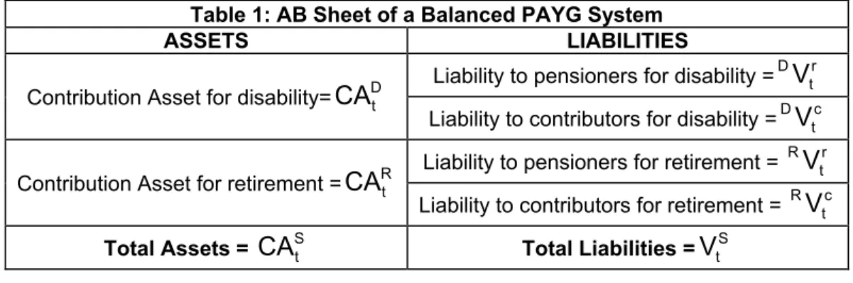
It can be described as a financial statement listing the pension system's obligations to contributors and pensioners at a particular date, with the amounts of the various assets (financial and through contributions) which back up these commitments. For Settergren (2009), Swedish reporting on financial status bears greater resemblance to the standard income statement and balance sheet of an insurance company. As we will see later, this balance sheet
1 An ABM is a set of predetermined measures established by law to be applied immediately as required according to the solvency indicator. Its purpose, through successive application, is to provide what could be called “automatic financial stability”, which can be defined as “the capacity of a pension system to adapt to financial, economic and demographic turbulence without legislative intervention”. For more details, see the papers by Barr & Diamond (2011), Vidal-Meliá et al (2009), Turner (2008), Börsch-Supan (2007), Penner & Steuerle (2007) and Lindbeck (2006).
2 A notional defined contribution scheme (NDC) is a pay-as-you-go scheme that deliberately mimics a financial defined contribution (FDC) scheme by paying an income stream whose present value over the person’s expected remaining lifetime equals his or her accumulation at retirement, and in doing so has many features of an FDC scheme. See for example the papers by Lindbeck & Persson (2003), Williamson (2004), Holzmann & Palmer (2006) Vidal-Meliá et al. (2006) and Whitehouse (2010).
3 Papers on the Swedish pension system include those by Palmer (2002), Sunden (2006), Pensionsmyndigheten (2011) and Chłoń-Domińczakel al (2012).
2 structure is perfectly valid for defined benefit pay-as-you-go systems (DB PAYG) in which the contribution rates for different contingencies are clearly separated.
The AB of the OASDI program4 has been compiled in US since1941. As Goss (2010) explains, it measures the difference in present value - discounted by the projected yield on trust fund assets - between spending on pensions and income from contributions over the next 75 years as a whole, expressed as a percentage of the present value of the contribution bases for that time horizon, taking into account that the level of financial reserves (trust fund) at the end of the time horizon reaches a magnitude of one year's expenditure.
The two models have very different characteristics and strengths. In the Swedish model the main accounting entries are developed from the principles of double-entry bookkeeping; and can briefly be summed up as showing the actuarial (im)balance in pension systems in understandable language in the shape of assets and liabilities and without needing to use explicit projections5. However, it can only be applied to the retirement contingency. The so- called US model, on the other hand, uses explicit projections to highlight future challenges to the financial side deriving basically from ageing, the expected increase in longevity and fluctuations in economic activity.
This paper will deal exclusively with the Swedish-type AB model, and especially the two concepts that make the balance possible: the system's average turnover duration and the contribution asset. These concepts initially appear in connection with NDCs, the general outline of which can be found in papers by Settergren (2001) and (2003), while in the paper by Settergren & Mikula (2005), both concepts are modeled in continuous time, giving theoretical support. The legal definitions and specific formulas applied in the Swedish system can be found in Pensionsmyndigheten (2011), while detailed explanations regarding the evolution of the system's solvency as determined from the balance can be found in the paper by Settergren (2012).
The search for valid expressions to apply to DB PAYG systems began with the paper by Boado-Penas et al (2008), continuing with that by Vidal-Meliá et al (2009), which in addition links it to the concept of the ABM. The paper by Vidal-Meliá & Boado-Penas (2013) obtains the analytical properties of the contribution asset and confirms its soundness as a measure of the assets of a PAYG scheme. However, all the papers cited limit themselves to the retirement
4 The Old-Age, Survivors, and Disability Insurance (OASDI) program in the United States provides a basic level of monthly income when insured workers become eligible for retirement and in cases of death or disability. The OASDI program consists of two separate parts that pay benefits to workers and their families - Old-Age and Survivors Insurance (OASI) and Disability Insurance (DI). Under OASI, monthly benefits are paid to retired workers and their families and to survivors of deceased workers, while under DI, monthly benefits are paid to disabled workers and their families. See the papers by BOT (2010), DeWitt (2010), Hoskins (2010) and Diamond & Orszag (2005).
5 See the paper by Boado-Penas & Vidal-Meliá (2012) for an in-depth study of the main differences and similarities.
3 contingency, which may be appropriate for defined contribution (DC) pension systems in which the contributory contingencies are clearly separated, but in DB PAYG systems there tends to be no clear separation between contingencies as far as contribution rates are concerned, and disability pensioners are often reclassified as retirement pensioners once they reach a certain age. Also, spending on disability pensions is hardly inconsiderable6.
The aim of this paper is to develop a theoretical basis for applying the Swedish AB to both the retirement and disability contingencies in a DB PAYG system. As mentioned earlier, there is a large gap in the literature which this paper hopes to fill, since so far nobody has looked at the possibility of compiling this type of AB from the integrated perspective of both retirement and disability contingencies, which are closely linked and account for a very high proportion of pension spending in DB systems.
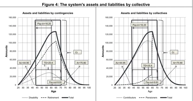
After this brief introduction, in Section 2 we develop a new expression for the system's average turnover duration in which both contingencies are included. In Section 3 the expressions obtained are applied using various reasonable assumptions to a numerical example representative of the system. The results for the system's assets and liabilities per contingency are also shown and special attention is paid to the phenomenon identified as pension reclassification. In Section 4 we list our main conclusions, and the paper ends with two appendixes in which we deduce some of the formulas used earlier.
2.- The contribution asset and the turnover duration in DB PAYG systems with two contingencies.
In this section we develop the concept of the contribution asset (CA)7 for a case in which the participants’ lives last (w-1-xe) periods, where (w-1) is the highest age to which it is possible to survive and xe is the age of entry into the system. In this case, A generations of contributors, (w-1-(xe+A)) generations of retirement pensioners and (w-2- xe) generations of disability pensioners coexist at each moment in time8.
6 In Spain at 1-1-2012, spending on contributory retirement pensions accounted for 67.95% of total spending on pensions, while disability pensions accounted for 11.39%, together totaling 79.34% of contributory spending. According to information provided by BOT (2011), spending on retirement pensions in the USA accounted for 63.19% of the total, with disability pensions - which are not subject to reclassification like they are in Spain - accounting for 16.40%, together totaling 79.59%.
7 Jackson (2004) proposed a financial statement for US Social Security prepared in accordance with the principles of accrual accounting, and based on the so-called “quasi asset”, an amount equal to the present value of excess revenues to be contributed by system participants over the additional benefits that they will accrue over the balance of their working lives. Valdés-Prieto (2005) also suggests using this “quasi asset”
(“hidden asset” in his terminology) as a valid asset for drawing up the AB sheet of a DB PAYG scheme.
8 We adopt the hypothesis that at the earliest age at which one can contribute, xe years, there are no disability pensioners. However, people become disabled throughout the period and start to receive a pension one year later, i.e. at age xe+1 años.
4 The process for obtaining the system's turnover duration (TD)9, its CA and a description of some of its characteristic features can be separated into 5 steps for the purposes of clarity:
1.-Description of the system and determination of the year in which it reaches a steady state10 (the contribution rates for both contingencies remaining stable in time and the system's financial equilibrium being maintained).
2.-Obtaining the analytical expressions for the system's liabilities from the actuarial point of view, distinguishing between contributors and pensioners, retirement and disability.
3.-Obtaining the analytical expression for the system's TD in the form of pay-in and pay-out.
4.-Obtaining the expression for the system's TD as the difference in the weighted average ages of pensioners and contributors.
5.-Obtaining the system's TD and CA as weighting for the TDs and CAs for each contingency.
2.1.-Description of the system and determination of the year in which it reaches a
“mature” state.
We use the case developed Vidal-Meliá & Boado-Penas (2013) in which the contribution base increases or decreases at an annual real rate of g, i.e. zero inflation is assumed, but with the additional assumptions that the population increases or decreases over time at an annual accumulative rate of γ affecting all groups of contributors equally, which means it must be assumed that real GDP and the wage bill also increase or decrease at rate G
=(1+g)·(1+
γ
)-1 and that pensions in payment increase or decrease at an annual rate of λ. The pension system's parameters are considered to be in a steady state. The contributor collective is open, i.e. the system has guaranteed a perpetual flow of new entrants.Both the age giving entitlement to retirement pension, “xe+A”, and the formula used for calculating retirement pension are constant, leading to a fixed replacement rate of size . As regards disability pension, it is supposed that initially the ages that give entitlement are to be found in age interval [xe, xe+A-1]11 and that for each age within that interval the calculation formula is a percentage (or adjustment factor) of the wage base. The age interval is later widened to [xe +1, w-1].
9 Lee (1994) began the formal development of the TD and described a framework to organize, summarize, and interpret data on transfer systems and the life cycle. Other pioneering papers which arrive at similar frameworks are Arthur & McNicoll (1978) and Willis (1988).
10 It is usual to replace the qualifying condition “steady state” with the condition “mature”.
11 Indeed a person of xe years may become disabled after having paid contributions, and therefore starts to receive disability pension at age xe+1 years. Similarly, a person of xe+A-1 years may become disabled at that age after contributing and will therefore receive benefit for being disabled at age xe+A years.
5 Diagram 1 shows the relationships (transitions) between the various collectives (states) that will be separated in the model:
The difference between this and the model found in Vidal-Meliá & Boado-Penas (2013) is that a new state - disability - is introduced, along with the new relationships shown in the diagram by dotted lines.
The demographic-financial structure at any moment “t” from the system's inception is given by:
1.-Age:
y) (disabilit ages ' Pensioners
e e
e e
e
t) (retiremen ages ' Pensioners
e e
ages rs' Contributo
e e
e e
1 - w ....
1,...
A x A, x 1, A x ...., ...
2, x 1, x
1 - w ....
1,...
A x A, x 1, A x ...., ...
2, x 1, x , x
1.
We adopt the assumption that the contributor cannot contribute and receive pension in the same year. However, if an individual becomes disabled at contribution age xe +k [xe, xe+A- 1], the corresponding disability pension payable will be xe +k+1 [xe+1, xe+A].
2.- Number of contributors by age at time t:
Contributor (c) Diagram 1.
Contribution, disability, retirement and death
Disabled (d)
Deceased (dc)
Retired (r)
xe + k ≤ xe + A-1 xe + A-1
xe + k ≥ x
e + A xe + k ≤ xe + A-1
xe + k ≥ x
e + 1
6
N (1 γ), N (1 γ) ,...,N (1 γ)
...,N ...
...
...
N , N ,
t e
t e
t e
e e
e
0) 1, A (x 0)
1, (x 0)
, (x
t) 1, A (x t)
1, (x t) , (x
2.
where N(xek,t)N(xe ,t) kRxe , with kRx
e being the stable-in-time ratio between the number of individuals of age xe and xe+k years, which can be increasing or decreasing and can also be expressed by means of probabilities k xp
e. Stable ratios or probabilities include the decrements due to death and disability associated with each age, with the possibility of a return to active life not being considered (practical disability model). It is a different matter when it comes to considering decrements or new entries due to migratory movements, these being included in parameter
γ
.3.- Average wage (average contribution base) by age at time t:
y (1 g), y (1 g) ,............,y (1 g)
...,y ...
...
...
y , y ,
t e
t e
t e
e e
e
0) 1, A (x 0)
1, (x 0)
, (x
t) 1, A (x t)
1, (x t) , (x
3.
4.- Number of disabled in age interval [xe+1 , xe+A] at t = 1
1 - A x x 1 - 0) A , 1 (x - A 1) x
A,
(x (x A-1,0)
1 - k x x 1 - 0) k , 1 (x - k 1) x
k,
(x (x k-1,0)
1 x 1 x
x 0) 1, (x 1) 2,
(x (x ,0)
1) x 1,
(x (x ,0)
e e e
e e e
e e e
e e e
e e e
e
e e
e e e
i N p
N i I
..., ...
...
...
, i N p
N i I
..., ...
...
...
, i N p
i N
I
, N i
I
4.
where x k-1
i e is the probability that an individual of age xe+k-1 will suffer permanent disability without being able to return to active life, (x k,1)
I e is the number of people who become disabled12 in year t of age xe+k, and Ix k-1
p e is the probability of survival of a disabled person at age xe+k-1, which may be different from that for the active population.
For t ≥ 2 and age interval [xe+1 , xe+A], we need to consider two types of disabled
12 Become disabled as far as the system is concerned, because their disability really began in the previous period [0, 1).
7 people: those aged xe+k years who became disabled in the current year, Nx k, t
I e , and those whose disability began earlier or survivors aged xe+k years who continue from previous years,
s t k, xe
I , whose evolution will depend on survival probabilities pIxek-1. The structure for the number of people who became disabled during the year in question is always given by:
1 γ
I
i γ) p
N (1 γ) i
N (1 i
N I
...., ...
...
,...
γ 1 I
i γ) p
N (1 γ) i
N (1 i
N I
...., ...
...
,...
γ 1 I
i γ) p
N (1 γ) i
N (1 i
N I
, γ 1 I
γ) i N (1
i N
I
1 - t 1
A, x
1 - A x x 1 - A 0
, x 1 - A x 0
, 1 - A x 1 - A x 1 - t , 1 - A x N
t A, x
1 - t 1
k, x
1 - k x x 1 - k 0
, x 1 - k x 1
, 1 - k x 1 - k x 1 - t , 1 - k x N
t k, x
1 - t 1
2, x
1 x x 0
, x 1 x 0
, 1 x 1 x 1 - t , 1 x N
t 2, x
1 - t 1
, x x 0
, x x
1 - t , x N
t 1, x
e
e e 1 - t e
e 1 - t e
e e
e e
e e 1 - t e
e 1 - t e
e e
e e
e e 1 - t e
e 1 - t e
e e
e
e e 1 - t e
e e
e
1
5.
After xe+A+1 years all the disabled in the system are by definition considered survivor disabled because, once the state of activity disappears, nobody can become disabled for the purposes of the system. Therefore, and always for t ≥ 2, as far as the continuing disabled are concerned a distinction has to be made between two age intervals, [xe+2, xe+A]13 and from xe+A+1 years onwards. The structure of the survivor disabled in [xe+2, xe+A] incorporates all those who became disabled in successive earlier periods and have survived. In general,
p γ
1 I
p I
p γ 1 I
p γ 1 I
p I
p γ 1 I
p p
I p
γ 1 I
p I
I p
I I
I s x s - k s k - 1 - 1 t
- k
1 t - k 1, Máx s
1 s, x
I 3 - k x 3 3 - t 3, - k x I
2 - k x 2 3 - t 1
2, - k x I
1 - k x 2 - t 1
1, - k x
I 2 - k x 2 2 - t 2, - k x I
1 - k x 2 - t 1
1, - k x
I 1 - k x I
2 - k x 2 - t 2, - k x I
1 - k x 2 - t 1
1, - k x
I 1 - k x S
1 - t 1, - k x N
1 - t 1, - k x I
1 - k x 1 - t 1, - k x S
t k, x
e e
e e
e e
e e
e e
e e
e e
e e
e
e e
e e
e e
6.
The total number of disabled for each age in t can be calculated by:
13 In k = 1 the disabled are always newly disabled as they come from age xe in t-1, and therefore I(xe +1, t)
= IN(xe +1, t).
8
k
t-1-k s k-s Ix s1 t - k 1, Máx s
1 s, x t
k,
xe I e 1 γ p e
I
7.This type of structure is maintained until all the disabled people who began in t = 1 have disappeared, which means that t = w-xe, and therefore from here onwards in all this disability band we get k < t, and so Max
1,k-t1
1.From xe+A+1 years onwards no more new disabled people are taken into account, and so for age interval [xe+A+1, w-1], i.e. k {1, w-1- (xe+A)}, we get:
I A x k A
1 k t - A 1, Máx s
I s x s - A s A k - t 1)
s, (x I
A x k k) - t A, (x t) k, A
(xe I e p e I e 1 γ p e p e
I
1 8.The demographic framework above implies that the age-wage structure only undergoes proportional changes. The slope of the age-wage structure is constant.
The annual retirement pension is PRx A,1 β YC, 0
e , which is a set percentage, β, of
the average contribution bases taking into account all the years (A) contributed, and pensions in payment are indexed at an annual rate of λ. It will also be assumed that contributions and benefits are payable in advance.
If k [1, A] the initial annual disability pension (in t=1) is Ix k,1
P e , the pension amounts for the newly disabled in t ≥ 2 and k [1, A] are calculated according to the following formula:
Ix k,t PIx k,1
1 g
t-1 bIk yx k,1
1 g
t-1P e e e 9.
because PIxek,1 is considered to be a variable percentage, bIk, of the contribution base of all the wages that contributions had been paid on, k years, at the age of becoming disabled,
k
y y
1 - k
0 h
) 1 h k h, x ( 1
k, x
e
e
, therefore: Ix k,1 Ik x k,1
e
e b y
P
The amounts of the disability pensions for survivors from previous periods, PSxek,t, xes, also in t ≥ 2, k [1, A] and being xe+s, with
s Max 1, k - t 1 , , k - 1
, the age at which the disability first began, would be obtained in accordance with this formula:9
Sx k,t, x s PIx s,1
1 g
t-k-1 s
1 λ
k s bIs yx s,1
1 g
t-k-1s
1 λ
k sP e e e e
10.
It can in fact be seen that for each period t and for each age k there is a vector 1x(k-s) of old pension amounts, i.e. of as many components as the difference between the age used for calculating the benefit, k, and the age at which it first came into payment, s.
The disability pensions for ages [xe+A+1, w-1-xe-A) are all for survivors as no newly disabled are considered, but by following them back to age xe+A they may come from newly disabled at that age or from survivor disabled from previous ages (a vector of 1x2), in such a way that:
I Sx A,t -k
kk - t A, x I
t k, A
x P ,P 1 λ
P e e e 11.
but because, following [10.], Sx A,t -k
P e is going to depend on the age at which the disability originally began, then we get
s Max 1, A 1 t k , , A - 1
, and once we considerIxe A,t -k
P , the final formula for
s Max 1, A 1 t k , , A
will be:Ix A k,t, x s PIx A,1
1 g
t k A 1s
1 λ
A k s bIs yx s,1
1 g
t k A 1s
1 λ
A k sP e e e e
12.
and like what we said for equation [11.], Ix A k,t
P e is also a row vector, in this case of 1x(A-1- s) with s
Max
1, A1tk
, A
.In this scenario, the stability of the total contribution rate (θI+θR) that ensures equality between contribution revenue and pension expenditure depends on the stability of the dependency ratios of both contingencies. For the retirement contingency, the contribution rate from year “w-xe-A”, counting from the system's inception, can be considered constant from the actuarial point of view because from that moment the dependency ratio (dr) stabilizes.
10
R D 1 t
A
0 k
1) +k, (x 1 A x w
0 k
1) k, A (x
1 A
0 k
1) +k, (x
1 A x w
k
I s x s - k A A
1 s
1) s, I (x
s x s - k A
1 k
k
1 s
1) s, (x
rs contributo
1 A
0 k
1) +k, (x
pensioners retirement
1 A x w
0 k
1) k, A (x )
( ages) t (retiremen disabled
1 A x w
1 k
t) k, A (x )
( ages) (working disabled
A
1 k
t) k, (x t
dr C dr
R C D C
R dr D
...
dr N
N (1 γ)
N
γ) p I (1
I (1 γ) p
C γ) N
(1
R
N (1 γ)
D I
D I
dr
e e
k e
e e
e s
k - A - e e
s k e
t e 1
t
t e
k 1 t e
r t e
e l
t
e
1
13.
The same moment “w -xe-A” can be considered for disability pensioners from retirement age onwards, but for continuing disability pensioners these pensions end up being dependent on pensions from before retirement age, and so in fact the ratio between contributors and disability pensioners does not stabilize until “w-xe-1”. Given that it is clear that w-xe-1 > w-xe-A and it is assumed that t >= w-xe-1, the contributor/pensioner ratio must be stable because all three collectives evolve (growing or shrinking) at a rate exactly the same as
γ
.From that year onwards the system is “mature” and, as can be seen in Appendix 1, the expressions for the contribution rates for both contingencies (retirement/R and disability/D), which can be separated, are:
R R
1 1 t
A
0
k (x +k,1) (x +k,1) 1 k
A x w
0 k
1) k, A 1) (x
A, (x
base on contributi Aggregate
1 A
0
k (x +k,1) (x+k,1) benefits retirement on e Expenditur
1 A x w
0 k
1) k, A (x 0
C, R
t θ ... θ
N y
G 1
λ N 1
P N
y G) (1
N (1 G) (1 λ)
β Y θ
e e
e
e e
e e
t e
k k t
e
14.
with
A y Y
1 A
0 k
) 1 k A k, x ( 0
C,
e
, the average contribution base taking into account all the years (A) contributed, and consequently βYC,0P(xeA,1), and also in the case of disability:
11
C,0
t-11 - t 1)
t) 1g βY 1g
A, (x A,
(xe P e
P ; 15.
while the contribution rate for the disability contingency is:
D base on contributi Aggregate
1 A
0
k (x+k,1) (x +k,1)
ages) t (retiremen benefits disability on e Expenditur 1
A - x - w
1 k
A
1 s
I s x s - k A s - k A 1
s, x I
1 s, x ages)
(working benefits disability on e Expenditur
I s x s - k s - k 1
s, x A
1 k
k
1 s
I 1 s, x
D t
θ ...
N y
G p 1
λ I 1
P G p
1 λ I 1
P
θ
e e
e
e e
e e
e e
16.
If the system's average disability pension is considered to be:
γ) p I (1
I (1 γ) p
G p 1
λ I 1
g) P (1
p γ)
I (1 I (1 γ) p
G p 1
λ I 1
g) P (1
P
pensioners Disability
1 A x w
1 k
I s x s - k A A
1 s
1) s, I (x
s x s - k A
1 k
k
1 s
1) s, (x
ages) t (retiremen benefits disability on e Expenditur
1 A x w
1 k
A
1 s
I s x s - k A s - k A 1
s, x I
1 s, x 1
t
pensioners Disability
1 A x w
1 k
I s x s - k A A
1 s
1) s, I (x
s x s - k A
1 k
k
1 s
1) s, (x
ages) (working benefits disability on e Expenditur A
1 k
k
1 s
I s x s - k s - k 1
s, x I
1 s, x 1
t Dt
e
e s
k - A - e e
s k e
e
e e
e
e
e s
k - A - e e
s k e
e e
e
17.
then the system's average retirement pension, taking into account 15., can be expressed as: