February 14, 2022 1
Asymptotic study of premixed flames in inert porous media layers of finite width: parametric analysis
of heat recirculation phenomena
Vadim N. Kurdyumov
1, Daniel Fern´andez-Galisteo, Carmen Jim´enez
Department of Energy, CIEMAT, Avda. Complutense 40, 28040 Madrid, Spain
Abstract
In this paper, we present an investigation on super-adiabatic premixed flames in an inert porous medium layer of finite length. The combustion process is modeled by a one-step Arrhenius kinetics in which density variations are taken into account. The asymptotic case of large ratio of thermal conductivities of solid to gas phases and the high activation energy limit are explored. The results obtained for these limiting cases are compared to those for finite values of these parameters. The use of the flame sheet model allows us to obtain steady-state solutions in an analytical form thus facilitating the parametric analysis.
The investigation focuses on the phenomenon of multiplicity of steady-state solutions.
It is shown that two or three (nontrivial) steady-state solutions are possible, depending on the flow rate intensity. The critical values of the parameters for the existence of multiple solutions are also determined. The stability of the obtained solutions is finally investigated by means of time-dependent simulations.
1 Introduction
Although the fundamental ideas related to super adiabatic combustion have more than fifty years of history [1–3], attention to this topic is not waning, but only increasing. A key characteristic of these devices is the ability to achieve a temperature in the combustion zone that exceeds the temperature obtained from a simple enthalpy balance between the initial mixture composition and the final products. This makes it possible to use them for various purposes. Among them, one can list the after burning of harmful impurities in gases for their final disposal or the extrac- tion of electrical energy from a micro-combustion device in conditions of remoteness from other sources of energy. Detailed reviews of these micro-combustion devices and their applications can be found in multiple publications, see [4–11].
1Corresponding author
@2022 This manuscript version is made available under the CC-BY-NC-ND 4.0 license: http://creativecommons.org/licenses/by-nc-nd/4.0/
A typical design used for micro combustion devices is a system of channels in which flows are established in a countercurrent pattern in adjacent channels. The width of the channels should be comparable to the thermal width of the flame, which is necessary to ensure enough heat transfer between the channels. This makes it possible to enhance the effect of heat recirculation, by which part of the heat energy does not leave the system and is used to preheat the incoming fresh mixture.
Another way for organizing heat recirculation is the use of an inert porous medium to in- crease the heat exchange between the hot combustion products and the cold mixture entering the device. In this case, the requirement of narrow channel width disappears, which obviously reduces the restrictions on the maximum values of the flow rate through the device.
The interaction of premixed flames with inert porous media has been studied in several inves- tigations applying asymptotic, numerical and analytical methods. Four different configurations can be identified in these studies, depending on the porous medium geometry, the flow direc- tion and the flame position. In the first configuration [12, 13], the porous layer was assumed to be semi-infinite, and fresh combustible gas was supplied from the gaseous half-space. In this configuration combustion takes place inside the porous medium at a finite distance from the gas-porous layer boundary and a single steady flame position exists.
In [14–17], the structure of a flame motionless relative to an infinite inert porous medium was investigated. This state corresponds to a unique, particular value of the filtration velocity of the incoming gas. In all the cases mentioned above [12–17] the maximum temperature in the flame exceeds the adiabatic flame temperature value.
In [18–21], the studied configuration was that of a premixed flame in a gas flow emerging from a semi-infinite porous media with a fixed (cold) temperature. In this case the flame is located at a finite distance downstream from the porous layer edge. It was shown that the thermal interaction of the flame with the upstream porous layer can promote oscillatory dynamics even for flames with unity Lewis number.
In the last configuration, the flame structure inside a porous layer of finite length was studied, see [17, 22–24]. Contrary to the previous situation, the temperature of the porous layer is not fixed and it has to be found as a part of the solution. In this configuration, two steady-state solutions with two different flame positions situated inside the porous layer were identified.
These studies were also carried out using asymptotic [22], numerical [23, 24] and analytical methods [17]. Interestingly, in [17] where the configurations with finite and infinite porous layer width were considered, it was shown that there is a maximum length above which the finite
length layer is equivalent to an infinite layer from the point of view of the efficiency of the recirculation.
The present investigation revisits the last configuration and considers the structure, stability and dynamics of a flame in an inert porous layer of finite length. Anticipating the presentation of the results, and also in order to emphasize the novelty of the present study, we indicate that in addition to the two solutions reported previously, the existence of a third possible flame mode is predicted for certain values of the parameters. Additionally, we investigate the stability of the steady state solutions, which, to the best of our knowledge, has not been studied before, and demonstrate that two of the three modes are stable.
It is interesting to note that a similar pattern with two stable steady-states was reported re- cently in [25], where a porous burner of a different and more complex type was studied ex- perimentally. Nevertheless, the presented work does not set the task of modeling this type of burners, which would require a particular investigation.
The analysis is carried out under the physical assumption that the value of the thermal con- ductivity of the solid phase is much higher than the thermal conductivity of the gas. The steady- state analysis is carried out in an analytical form under the natural assumption for combustion of a high activation energy. It should be noted that in the previous studies (with the exception of [24]) the assumption of a constant gas density was adopted. Unlike this, changes in gas den- sity with temperature which affect the reaction rate are taken into account in the present study.
The obtained asymptotic results are compared with the numerical solutions for finite values of these parameters.
The aim of this work is not to study a specific case, but rather to explore general trends in the structure of a flame stabilized in a porous medium of finite length from an asymptotic point of view. The article is structured as follows. Section 2 presents the mathematical formulation of the problem. The asymptotic assumptions adopted in the study are discussed in Section 3, where the corresponding analytical solution to the problem is also constructed. Section 4 describes the solution to the problem for finite values of the Zel’dovich number, which is then compared with the analytical solution. Section 5 is devoted to a discussion of the results.
2 General formulation
Consider a combustible gaseous mixture at initial temperature T0, density ρ0, and fuel mass fractionY0flowing through an inert porous layer of finite widthL. The gas velocity far upstream
x
0 L
U0
porous medium
gas gas
flame Y θ
θ,Y
xf
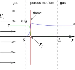
Figure 1: Sketch of the problem.
the porous layer is U0. The configuration sketch is shown in Fig. 1. Following the standard continuum model for a porous medium (see [26], for example), we denote asU the gas seepage velocity inside the porous medium and the gas velocity outside the porous layer. This magnitude ensures the continuity of the gas mass flow rate,ρ U, through the gas-porous medium boundary.
Inside the porous layer, a two-temperature continuous model is used, in whichT andTs denote the temperatures of the gas and the solid phase, respectively. It is assumed that the motion is spatially one-dimensional and all variables are functions of a single spatial coordinate x and timet.
The combustible mixture undergoes a chemical reaction modeled by a global irreversible step F + O → P, where F, Oand P denote the fuel, the oxidizer and the products, respec- tively. Assuming that the mixture is lean in fuel, the oxidizer mass fraction remains nearly constant. Generalization of the problem to cases of non-lean mixtures will be done some- where else. The amount of fuel consumed per unit volume of gas and per unit time is given by Ω = BρnY exp(−E/RgT) , where B is a pre-exponential factor, ρ is the density of the mixture, Y is the fuel mass fraction, E is the overall activation energy and Rg is the univer- sal gas constant. The Arrhenius kinetics frequently used to simulate a combustion process is a simplification of more complex multicomponent kinetics. There is no unanimous agreement in the combustion literature concerning the power n, and values 0, 1 and 2 for n have been used used in different studies. Formally, n = 0 corresponds to the diffusion-thermal approxi-
mation when density changes are neglected. If we consider in a simplified way the process of a binary chemical reaction, when one fuel molecule meets one oxidizer molecule, the collision frequency should be proportional to the concentrations of each mixture component at a given point of space. Thus, perhaps the most reasonable compromise is indexn = 2.
For simplicity, we will assume constant values for the constant-pressure gas and solid heat capacities,cg andcs, the conductivities,λg andλs, the mass fuel diffusion coefficient, ρD, the solid phase density,ρs, as well as the isobaric assumption. While some research has been done relaxing this assumption, it will be reported elsewhere in order not to overwhelm the presen- tation. Here, we can report that taking into account variable properties leads only to relatively small changes in the quantitative results without changing the qualitative behavior of the curves.
The porosity of the layer is denoted asϕhereinafter. Although this value for porous ceramic materials is about0.6÷0.8, in this study a wider range for porosity is considered, ϕ = 0.4÷ 0.8. Heat exchange between the gas and solid phases follows a linear law, namely, the amount of energy that is transferred from one phase to another per unit volume and per unit time is proportional to the temperature difference, Hv(T −Ts). There is an experimental correlation estimate suggested in [30] for the coefficient of volumetric heat transfer,Hv, between phases:
Hvd2p λg =
(
0.0426 + 1.236 L/dp
)
Red, (1)
wheredp is the characteristic pore size and Red = ρudp/ϕµ, with µthe viscosity. According to [30], this correlation formula is valid in the interval2 < Red < 836. The same expression was used in the numerical studies presented in [24].Although Eq. (1) can raise questions, since it includes the layer lengthL (the global characteristic) to correlate the local characteristic of the process (at a given point in space), and also does not include the thermophysical properties of the porous material, it will be used here to estimate the coefficient of volumetric heat transfer between phases. In the present study, this value is taken constant when carrying out parametric analysis. Anticipating the analytical procedure to be developed, a generalization to account for the flow-rate dependence for this quantity can be easily made.
When selecting characteristic scales for a combustion problem, it is convenient to use the characteristic values corresponding to a planar adiabatic flame for a given mixture composition.
In the following, the burning velocity of the planar (gaseous) flameSL, the thermal flame thick- ness defined as δT = DT/SL, with DT = λg/ρ0cg the thermal diffusivity, and the adiabatic flame temperatureTa=T0+QY0/cg, withQthe total heat of combustion per unit mass of fuel, are used to specify the non-dimensional parameters. Non-dimensional temperatures defined as
θ= (T−T0)/(Ta−T0)andθs= (Ts−T0)/(Ta−T0)are introduced in the following, whileSL, Y0andρ0are used to normalize the velocity, the fuel mass fraction and the density, respectively.
Let’s introduce the following functions Φ(x) =
{
ϕ, 06x6ℓ ,
1, x <0, x > ℓ , B(x) = {
b, 06x6ℓ ,
0, x <0, x > ℓ , (2) whereϕ represents the porous layer porosity andb is the dimensionless effective heat transfer coefficient between the gas and solid phases, defined as a function ofHvfurther below. In what follows, a two-temperature continuum model similar to that used, for example, in [14–16] is applied.
It is well known that possible heat losses with the external environment can affect the over- all map of possible solutions. Accounting for these effects requires taking into account some additional geometric characteristics of the burner, such as, for example, the transverse width of the porous layer. For the sake of simplicity, heat losses will be assumed to be negligible in the present study. This reduces the number of parameters thus facilitating the obtention of more general results within a simplified model.
The well-known conservation equations of the mass, the fuel mass and the gas thermal en- ergy for both a space occupied by a porous medium (Φ =ϕ) and a porous-free space (Φ = 1) are written in the form
Φ∂ρ
∂t +∂(ρu)
∂x = 0, (3)
Φρ∂Y
∂t +ρu∂Y
∂x = 1 Le
∂
∂x (
Φ∂Y
∂x )
−Φω , (4)
Φρ∂θ
∂t +ρu∂θ
∂x = ∂
∂x (
Φ∂θ
∂x )
+ Φω−B(θ−θs). (5) These equations are considered for−∞ < x < ∞. The corresponding equation for the solid thermal energy becomes
(1−ϕ)ξ∂θs
∂t = (1−ϕ)Λ∂2θs
∂x2 +b(θ−θs), (6)
considered for0 < x < ℓ. The above equations are supplemented by the isobaric equation of state for the (ideal) gas
ρ(1 +qθ) = 1. (7)
The dimensionless reaction rate is written as ω= β2
2Le u2p(1 +q)nρnY exp
{ β(θ−1) 1 +q(θ−1)/(1 +q)
}
. (8)
The boundary conditions for the velocity, the gas density, the temperature and the fuel mass fraction are described by fixing quantities far upstream and applying weak conditions far down- stream
x→ −∞: u−m=ρ−1 =Y −1 = θ= 0;
x→ ∞: ∂Y /∂x=∂θ/∂x= 0. (9)
The conditions at the planes separating the porous layer and gas situated atx= 0andx=ℓ are expressed in the form of the continuity of the mass fraction and the gas phase temperature together with their diffusion fluxes as follows
x= 0, ℓ : [Y] = [θ] = [Φ∂Y /∂x] = [Φ∂θ/∂x] = 0, (10) where[f] =f(x+)−f(x−). For the solid phase temperature we assume that
x= 0, ℓ: ∂θs/∂x= 0, (11)
thus neglecting, for simplicity, the radiation-thermal effects from the porous surfaces.
The following parameters appear in the above equations: the dimensionless flow rate,m = U0/SL , the dimensionless length of the porous layer, ℓ = L/δT, the Zeldovich number, β = E(Ta−T0)/RgTa2 , the Lewis number,Le =λg/cpρ0D, the heat release parameter,q = (Ta− T0)/T0 =Q Y0/cpT0, the dimensionless heat-exchange parameter,b=HvδT/ρ0cgSL, the ratio of thermal conductivities,Λ = λs/λg, and the ratio of the mass-weighted heat capacities of the solid and gas phases,ξ =ρscs/ρ0cg. One can see that for steady-state solutions, when∂/∂t≡0 is assumed, the value ofξbecomes irrelevant.
In theoretical studies related to combustion, the Zel’dovich number, β, is often used as a large parameter in asymptotic expansions, while the other parameters are assumed (formally) to be of the order of unity. It should be noted that in factβ and the heat release parameter,q, are related asβ = N q/(1 +q)2, where N = E/RgT0 is the dimensionless activation energy based on the initial temperature of the mixture. In what follows, we will use both quantities to characterize the flame, and the valueβ = 10will be used as a reference one corresponding to N = 72forq = 5. These values are standard in combustion modeling.
To estimate the dimensionless heat transfer coefficient between phases, b, we will assume thatL ≫ dp. In this case, it follows from Eq (1) thatb = 0.0426RedδT2/d2p. Thus, reasonable values forbare in the range0.03÷0.3. The specific value depends on the material of the porous layer and the composition of the combustible mixture. In this study, the valueb= 0.2is chosen as a reference value.
The factor up = SL/SLas included in Eq. (8) ensures that the non-dimensional speed of a planar adiabatic gaseous flame is equal to unityfor a given finite value of β. Here SLas is the asymptotic value of adiabatic laminar flame speed calculated atβ → ∞:
SLas=
√
2(λ0/cp)Leβ−2Bρn0−2(T0/Ta)nexp(−E/2RTa)
Precise calculation ofup requires the solution of the following eigenvalue problem dθ/dz =d2θ/dz2+ω, dY /dz =Le−1d2Y /dz2−ω,
z → −∞: θ =Y −1 = 0, z →+∞: θ−1 = Y = 0, (12) whereωis given by Eq. (8). For largeβthe eigen-value of Eq. (12) is of the form
SL/SLas= 1 +c1(Le, q, n)/β+O(β−2) +. . . ,
see [31]. When carrying out the asymptotic analysis forβ ≫ 1in the following sections, this value is equal to unity, in the leading approximation. However, when performing numerical calculations at finiteβvalues,up is computed numerically by a shooting method.
The use of the factorup makes it possible to generalize the results to more complex kinetics.
Indeed, for this it is only necessary to use the speed of a planar adiabatic combustion wave (e.g.
measured experimentally) and the adiabatic flame temperature (obtained from the balance of enthalpy of the initial and final products) in writing the dimensionless parameters.
The flame position, xf, is determined by the point at which the reaction rate reaches its maximum value, ω|x=xf = ωmax. From a general consideration of the governing equations, it can be obtained that for steady-state solutions the gas temperature far downstream is equal to the adiabatic one,θ(x → ∞) = 1. This trivial fact also follows from the energy conservation law in the absence of heat loss.
3 Asymptotic analysis
3.1 Limit Λ ≫ 1
The dimensional parameters describing the properties of the gas and solid phases differ by or- ders of magnitude. Typical magnitudes of thermal conductivities suggestΛ =λs/λg =O(103).
Thus, the limit ofΛ → ∞is considered below. Assuming (formally) that all remaining param- eters are of order unity, we expand θs in the form θs = θs(0) + Λ−1θ(1)s +. . .. To the leading
order, Eq. (6) is reduced to∂2θs(0)/∂x2 = 0. The boundary conditions given by Eq. (11) indicate thatθs(0)is a function of time only. After integrating Eq. (6) over the porous layer thickness and dropping the superscript, we have
(1−ϕ)ξdθs dt =b·
(1 ℓ
∫ℓ 0
θdx−θs
)
. (13)
A similar limit of the constant temperature of a porous medium was considered in [23], where the balance for this value was established by heating from the outside. The results obtained for Λ≫1are compared below with those for finite ratios of the thermal conductivities.
3.2 Limit β ≫ 1
The typical Zel’dovich number is large,β ≫1, leading to a narrow combustion zone, of order δT/β, within whichω >0. The standard treatment consists in replacing the spatially distributed kinetics given by Eq. (8) by an infinitely thin flame sheet,
ω =F(θf, G)·δ(x−xf), (14) whereδ(·)is the Dirac δ-function, G = −dθ/dx|x=xf+ denotes the temperature gradient just behind the flame sheet (at the burnt side) andθf is the flame temperature. The substantiation of this procedure should be referred to [31] where the method of matched asymptotic expansions was first applied to the problem of steady-state propagation of an adiabatic planar combustion wave. In that case θf = 1 and G = 0. The rigorous justification for this approximation for general unsteady cases (G ̸= 0) was suggested in [27]. In the recent study [28] an extension was made for transport properties variable with temperature and heat-losses. This δ-function approximation has been used many times in the past, mainly for analytical purposes.
An asymptotic analysis based on the method of matched asymptotic expansions gives F(θf, G) = µ(G)−1/2
(1 +qθf 1 +q
)2−n/2
·exp {β
2
(θf −1) (1 +qθf)/(1 +q)
}
, (15)
see [27, 28]. The value ofµin Eq. (15) is determined by considering the inner flame region. It leads to the classical problem first investigated by Li˜n´an in his pioneering asymptotic study of diffusion flames [29]. Finally, the dependence ofµonGcan be approximated asµ≈1−µ1G, whereµ1 = 1.344046was calculated numerically.
Anticipating the comparison of the results of asymptotic analysis with the results of nu- merical calculations with the spatially distributed kinetics, we can conclude that the effect of a nonzero value ofGis relatively small. Thus, the choiceµ≡1is made in present study leading toF =F(θf)in Eq. (15).
When considering an infinitely thin inner combustion region, the fuel mass fraction and temperatures must be continuous at the flame sheet,
[Y]x=xf = 0, θ|xf− =θ|xf+ =θf. (16) Integrating Eqs. (4)-(5) acrossx=xf gives the well-known jump conditions
Le−1[dY /dx]x=xf =F(θf), [dθ/dx]x=xf +Le−1[dY /dx]x=xf = 0. (17) For the temperature of the solid phase, integration of Eq. (6) aroundx=xf leads to
[θs]x=xf = [dθs/dx]x=xf = 0. (18) Obviously, Eq. (18) is satisfied automatically for cases withΛ≫1.
3.3 Steady-state asymptotic solutions
Consider steady-state solutions imposing ∂/∂t ≡ 0 in Eqs. (3)-(6). Eq. (3) leads to ρu = m satisfied everywhere. Thus, for time-independent solutions, the density changes affect only the reaction rate term given by Eq. (8), whereρnis a factor. It should be also noted that steady-state solutions are independent of the parameterξappearing as a factor in front of the time derivative.
Let us assume that0 < xf < ℓ. Consideration of the inner flame region by means of the matched asymptotic expansions method shows that the fuel leakage (mass fraction of unburned fuel behind the flame) is, at least, of the order ofβ−1. This effect is small in the first approxima- tion. Thus,Y = 0can be imposed behind the flame, forx > xf, and the steady-state solution of Eq. (4) is
Y =
1−exp{mLe(x−xf/ϕ)}, x <0, 1−exp{mLe(x−xf)/ϕ}, 0< x < xf.
0, x > xf.
(19)
Here the continuity of the mass fraction and its diffusion flux has been required atx= 0.
From Eqs. (17) and (19) it follows, that
m=ϕ·F(θf). (20)
0 5 10 15 20 0.8
1 1.2 1.4 1.6 1.8 2
m/ φ θ
fn=2 n=0 n=1
β =10, q=5
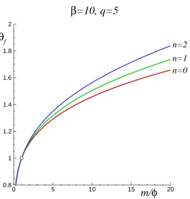
Figure 2: Dependence of the flame temperatureθf onm/ϕgiven by Eq. (21) for differentn, for β = 10,q= 5.
The same result can be obtained by integrating Eq. (4) overx within±∞. It should be noted that this relation is obtained only if the flame sheet is either inside the porous layer, whereϕ <1, or outside it, whereϕ= 1. The case when the position of the flame coincides with the boundary of the porous layer, forxf = 0or xf = ℓ, should be considered separately. This situation is discussed in the Appendix.
Equation (20) provides a direct relation between the flame temperature,θf, and the flow rate, m. Note that the function F is a monotonically increasing function of the flame temperature θf. This means that at a fixed value of m, a decrease in ϕ leads to an increase in the flame temperature. Finally, the flame temperature can be expressed as
θf = β(1 +q)2−q(4−n)Z
q2(4−n)Z (21)
with
Z =W
(β(1 +q) q(4−n) ·exp
{β(1 +q)−2qln(m/ϕ) q(4−n)
}) ,
whereW(·)is the Lambert function defined by the equationW(s)eW(s)=s. It is a multivalued function with an infinite number of branches such that for each non-zero value ofsthere is an
infinite number values ofW, most of them complex. Here the principal branch is used. The dependence ofθf onm/ϕis shown in Fig. 2 forβ = 10,q = 5for different values ofn. Note that for alln, Eq. (21) ensuresθf = 1form/ϕ= 1. Atm/ϕ >1, the flame temperature, if the steady-state exists, always exceeds unity (the adiabatic temperature value) and the combustion process is superadiabatic.
The gas temperature distribution outside the porous layer is θ=
{
A1exp (mx), x <0,
A2, x > ℓ, (22)
where A1 and A2 are unknown constants. Using this, Eqs. (10) allow to write the following conditions
x= 0 : mθ−ϕdθ/dx= 0;
x=L: dθ/dx= 0. (23)
The general solution on both sides of the flame-sheet becomes θ =θs+
{
C1ea1x+C2ea2x 0< x < xf,
C3ea1x+C4ea2x xf < x < ℓ , (24) where
a1,2 = m±√
m2+ 4ϕ b
2ϕ .
An additional condition required to determine the solid phase temperature is given by Eq. (13).
For time-independent cases, it takes the form
θs= 1 ℓ
∫ℓ 0
θ dx . (25)
This means that, in the absence of heat losses, the temperature of the solid phase coincides with the gas temperature averaged within the porous layer.
Five conditions for the temperature field, namely Eqs. (16), (23) and (25), serve to determine the unknown valuesCi, i = 1. . .4andθs. These equations are all linear with respect to these quantities. Despite the fact that these solutions are expressed in an analytical form, it makes no sense to write them down here because of their length. After finding them, analytical expressions for the gas temperature on both sides of the flame-sheet were substituted into
[dθ/dx]x=xf +F(θf) = 0. (26)
0 5 10 15 20 -1
0 1 2 3
0 5 10 15 20
-1 0 1 2 3
0 5 10 15 20
-1 0 1 2 3
x
fF
m=2.2783 m=2
m=2.5
θ
1θ
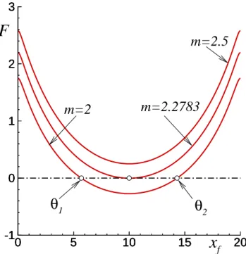
2Figure 3: Typical dependencies of the functionF onxf for different values ofm; all curves are plotted forq= 5,β = 10,n = 2,ℓ = 20,ϕ = 0.4,b = 0.2. The open circles for the curve with m= 2correspond to the solutions drawn in Fig.4.
The last step allows to find the flame positionxf. All these procedures were carried out using MAPLE facilities.
Based on the procedure described above, we can conclude that the steady-state results ob- tained within the framework of the flame sheet model are independent of the Lewis number.
First of all, Eq. (20) which determines the relationship between the flame temperature and the flow rate does not depend on the Lewis number. The Lewis number similarly does not appear in Eqs. (16), (23) and (25) required for findingCi, i = 1. . .4andθs, all functions ofθf. After finding analytical expressions for the temperature on both sides of the flame sheet, these expres- sions are substituted into Eq. (26), which as a consequence does not present a dependence on the Lewis number.
However, it should be noted that this independence of the results from the Lewis number, which expresses the ratio of diffusion to the thermal diffusivity of the gas, is the result of the adequate choice of the thermal flame width as a characteristic size of the problem. If the results are rewritten using dimensional variables, then they are clearly dependent on the fuel diffusion.
0 5 10 15 20 0
0.5 1 1.5
θs2 θ1
θs1
θ2 m=2
x
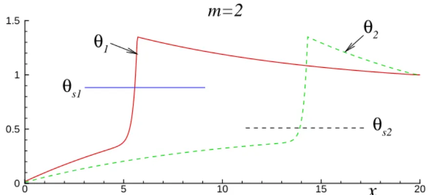
Figure 4: An example of temperature distributions (plotted within the porous layer only) for the lower (solid curve) and upper (dashed curve) solutions corresponding to the open circles on the curve withm = 2in Fig. 3. Temperature values for the solid phase are indicated by horizontal lines.
The final analytical expression to determinexf given by Eq. (26) (very long, also not repre- sented here) takes the form
F(xf;m, ϕ, b, N, q, n) = 0. (27) This nonlinear equation was used to evaluatexf numerically. Figure 3 shows typical dependen- cies of the functionF onxf for various values ofmwith other parameters fixed. These curves illustrate that Eq. (27) can have two, one or zero roots.
Let’s call the solutions corresponding to the lower and higher values ofxf as lower, θ1(x), and upper,θ2(x). These distributions are illustrated in Fig. 4 with solid and dashed lines, respec- tively. One can see that although both solutions correspond to the same value ofθf (according to Eq. (20), it depends onm/ϕonly), the solid phase temperatures for these two solutions are different,θs1 > θs2. These values are plotted in Fig. 4 with horizontal solid and dashed lines.
Note also that for any steady-state solution the temperature at the exit from the porous layer is equal to unity, as it should be, since there are no heat losses.
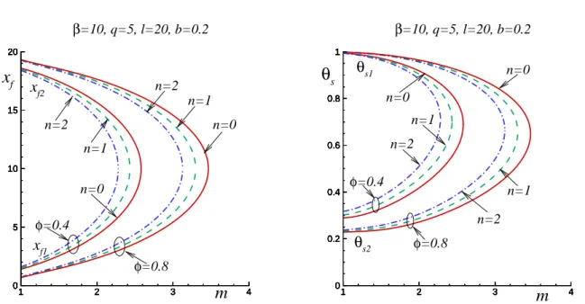
Figure 5 illustrates typical dependencies of the flame position xf (left plot) and the solid phase temperatureθs(right plot) as functions of the dimensionless gas flow ratem. The response curves are shown forn = 0,1and2. All other parameters are fixed atβ = 10, q = 5,ℓ = 20, b = 0.2and two values of ϕ. It can be seen that the curves have a familiar C-shape. When the flow intensity approaches the critical valuem = mc, the two solutions merge and disappear at m > mc. One can see that the influence of the parameter n is only moderately quantitative, leading to a decrease in the critical value,mc, with increasingn.
Figure 3 shows that when two roots merge into one, atm=mc, the functionF(xf, m, . . .)
1 2 3 4 0
5 10 15 20
1 2 3 4
0 5 10 15 20
1 2 3 4
0 5 10 15 20
1 2 3 4
0 5 10 15 20
1 2 3 4
0 5 10 15 20
1 2 3 4
0 5 10 15 20
m xf2
n=0 n=2
n=0
β=10, q=5, l=20, b=0.2
xf
xf1 n=2
n=1
n=1
φ=0.4
φ=0.8
1 2 3 4
0 0.2 0.4 0.6 0.8 1
1 2 3 4
0 0.2 0.4 0.6 0.8 1
1 2 3 4
0 0.2 0.4 0.6 0.8 1
1 2 3 4
0 0.2 0.4 0.6 0.8 1
1 2 3 4
0 0.2 0.4 0.6 0.8 1
1 2 3 4
0 0.2 0.4 0.6 0.8 1
n=2
n=2
m θs
θs2 θs1
β=10, q=5, l=20, b=0.2
n=0 n=0
n=1
φ=0.4 n=1
φ=0.8
Figure 5: Typical dependencies of the flame positionxf (left plot) and solid phase temperature θs(right plot) on the flow rate forn = 0,1and2.
becomes tangent to the horizontal axis. A rigorous determination of the critical values requires to solve a system of two equations with respect toxf andm,
F(xf, m, . . .) = 0, ∂F
∂xf(xf, m, . . .) = 0. (28) It was obtained that form = mc the critical flame position is situated exactly in the middle of the porous layer, namelyxf =ℓ/2always takes place.
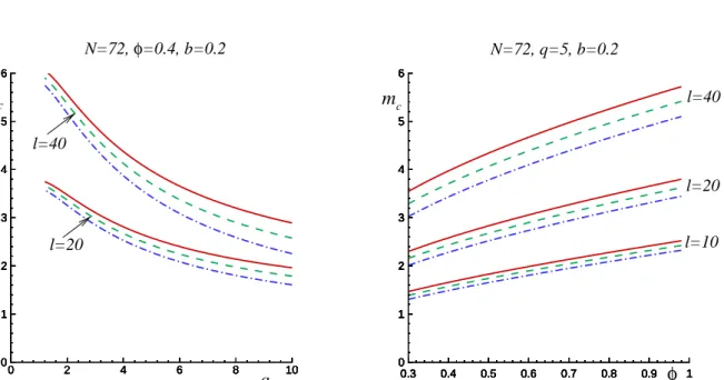
The existence of an analytical expression given by Eq. (27) facilitates greatly the parametric analysis of the solutions. Figure 6 illustrates the dependence of the critical value of the flow rate on the heat release parameterq (left plot) and on the porosity value (right plot) for layers with differentℓ. Note that the dimensionless activation energyN is fixed in the left figure, and not the Zel’dovich number calculated according toβ =N q/(1 +q)2. It can be seen that with increasing q(which leads to a decrease inβ), the critical value for the flow rate decreases. If the layer width ℓincreases, as can be seen in the right plot, the value of the critical flow rate increases.
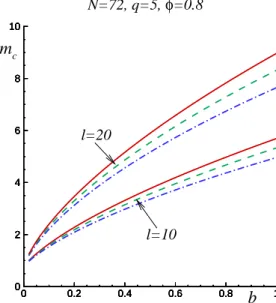
Figure 7 illustrates the dependence of the critical flow rate, mc, on the dimensionless heat exchange value between phases,b, for two porous layer widths and variousn. As expected, an increase in the heat transfer leads to an increase inmc.
The above dependencies show that the effect of heat recirculation, which increases the max- imum flow rate below which there are steady-state regimes, grows monotonically with an in- crease in the thickness of the porous layer, with an increase in the efficiency of heat exchange
0 2 4 6 8 10 0
1 2 3 4 5 6
0 2 4 6 8 10
0 1 2 3 4 5 6
0 2 4 6 8 10
0 1 2 3 4 5 6
0 2 4 6 8 10
0 1 2 3 4 5 6
0 2 4 6 8 10
0 1 2 3 4 5 6
0 2 4 6 8 10
0 1 2 3 4 5 6
q mc
N=72,φ=0.4, b=0.2
l=40
l=20
0.3 0.4 0.5 0.6 0.7 0.8 0.9 1
0 1 2 3 4 5 6
0.3 0.4 0.5 0.6 0.7 0.8 0.9 1
0 1 2 3 4 5 6
0.3 0.4 0.5 0.6 0.7 0.8 0.9 1
0 1 2 3 4 5 6
0.3 0.4 0.5 0.6 0.7 0.8 0.9 1
0 1 2 3 4 5 6
0.3 0.4 0.5 0.6 0.7 0.8 0.9 1
0 1 2 3 4 5 6
0.3 0.4 0.5 0.6 0.7 0.8 0.9 1
0 1 2 3 4 5 6
0.3 0.4 0.5 0.6 0.7 0.8 0.9 1
0 1 2 3 4 5 6
0.3 0.4 0.5 0.6 0.7 0.8 0.9 1
0 1 2 3 4 5 6
0.3 0.4 0.5 0.6 0.7 0.8 0.9 1
0 1 2 3 4 5 6
φ
mc l=40
l=10 N=72, q=5, b=0.2
l=20
Figure 6: Dependencies of the critical value for the flow rate, mc, on the heat release q (left plot) and the porosityϕ (right plot) for various values of the parameters; the solid, dashed and dash-dotted lines correspond ton= 0,1, and2, respectively.
0 0.2 0.4 0.6 0.8 1
0 2 4 6 8 10
0 0.2 0.4 0.6 0.8 1
0 2 4 6 8 10
0 0.2 0.4 0.6 0.8 1
0 2 4 6 8 10
0 0.2 0.4 0.6 0.8 1
0 2 4 6 8 10
0 0.2 0.4 0.6 0.8 1
0 2 4 6 8 10
0 0.2 0.4 0.6 0.8 1
0 2 4 6 8 10
N=72, q=5,φ=0.8 mc
b l=10
l=20
Figure 7: Dependencies of the critical value for the flow rate,mc, on the heat exchange coeffi- cientbfor various values of the parameters; the solid, dashed and dash-dotted lines correspond ton = 0,1, and2, respectively; all curves plotted forϕ = 0.8.
between the gas and solid phases or with an increase in the porosity. However, an increase in thermal expansion q leads to a decrease of the maximum flow rate. It should be remembered
0 0.2 0.4 0.6 0.8 1 0
0.5 1 1.5
0 0.2 0.4 0.6 0.8 1
0 0.5 1 1.5
0 0.2 0.4 0.6 0.8 1
0 0.5 1 1.5
0 0.2 0.4 0.6 0.8 1
0 0.5 1 1.5
0 0.2 0.4 0.6 0.8 1
0 0.5 1 1.5
0 0.2 0.4 0.6 0.8 1
0 0.5 1 1.5
β=10, q=5, l=20, b=0.2
m xf
φ=0.8 φ=0.4
0 1
20
0 1
20
0 0.2 0.4 0.6 0.8 1
18.5 19 19.5 20
0 0.2 0.4 0.6 0.8 1
18.5 19 19.5 20
0 0.2 0.4 0.6 0.8 1
18.5 19 19.5 20
0 0.2 0.4 0.6 0.8 1
18.5 19 19.5 20
β=10, q=5, l=20, b=0.2
m xf
φ=0.8 φ=0.4
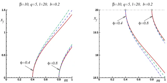
Figure 8: Flame position as a function of m for ϕ < m < 1 for the lower (left plot) and upper (right plot) branches plotted forϕ = 0.4and0.8; the solid, dashed and dash-dotted lines correspond ton = 0,1, and2, respectively.
that the flame temperature, θf, which depends only on the flow rate divided by the porosity coefficient, see Eq. (20), always exceeds the adiabatic temperature of the mixture in these cases.
3.4 Effect of flame stabilization by a porous layer
For all the cases presented above, the upstream gas flow rate was chosen to be greater than the planar flame propagation speed, m = U0/SL > 1. Obviously, for these cases, upstream flame propagation does not occur. However, if ignition takes place at x > ℓ, then there is a time-dependent solution in the form of a combustion wave propagating downstream at a speed v = m −1 relative to the porous layer. In the same way, when the dimensionless flow rate is less than one, m < 1, there is also a time-dependent solution of Eqs.(3)-(6) describing the combustion wave propagation towards negativexwith a negative speed,v =m−1.
A parametric analysis of Eq. (27) showed that form <1, in addition to the solutions in the form of a traveling wave, there are also steady-state solutions with the flame position located inside the porous layer. Figure 8 shows the dependence ofxf on the flow rate for the lower (left plot) and upper (right plot) solutions drawn for two values of ϕ = 0.4 and 0.8 and values of n = 0, 1and2. It can be seen that, regardless ofn, the critical value m∗ at which the position of the flame is situated at xf = 0 or xf = ℓ is equal to ϕ. In both cases,θf = 1, as follows
-5 0 5 10 15 20 25 0
0.5 1 1.5
-5 0 5 10 15 20 25
0 0.5 1
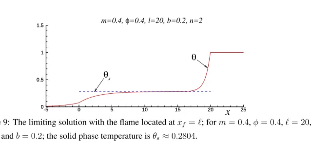
1.5 m=0.4,φ=0.4, l=20, b=0.2, n=2
x
θs
θ
Figure 9: The limiting solution with the flame located atxf =ℓ; form= 0.4,ϕ= 0.4,ℓ= 20, n= 2andb= 0.2; the solid phase temperature isθs ≈0.2804.
from Eq (20). The same behavior for the response curves was observed for other values of the parameters.
The limiting solution with the flame position atxf = 0is trivial, θ =
{ ex, x <0,
1, x >0, θs= 1. (29)
This can be easily verified by substituting Eq. (29) into the governing equations. Obviously, this solution is independent of other parameters. The temperature of the solid phase is exactly equal to the temperature of the gas behind the combustion zone.
For the other solution corresponding to the flame situated atxf =ℓ, an example of temper- ature distributions in the gas and solid phases is shown in Fig. 9 plotted form = 0.4,ϕ = 0.4, ℓ = 20, b = 0.2. In this case, the solid phase is heated to a certain temperature less than the temperature behind the combustion zone, which is also equal to unity. The gas temperature is less thanθsat the beginning of the porous layer and exceedsθsat the end of the layer. The value of the temperature of the solid phase depends on the parameters. Anticipating the results of time-dependent simulations, the upper branch solutions (corresponding toℓ/2< xf < ℓ) result to be unstable. However, the temperature distribution shown in Fig. 9 represents the asymptotic solution for the third steady-state mode described below, see also Appendix, when the flame is located at the trailing edge of the porous layer. This solution is stable.
Although this effect can be explained by an increase of the local gas velocity between the pores (due to a decrease in the average free area), it is interesting that the critical value of the gas flow rate for flame stabilization, mc = ϕ, does not depend on other parameters such as b, for example, within the framework of the model under study. In this case, the temperatures of
1 2 3 0
5 10 15 20
1 2 3
0 5 10 15 20
1 2 3
0 5 10 15 20
1 2 3
0 5 10 15 20
1 1.5 2 2.5 3
0 5 10 15 20
m x
fΛ=20
Λ=1000
Λ=100 Λ=
∞
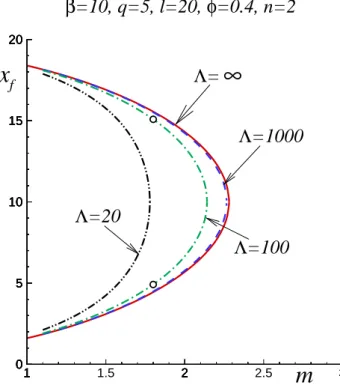
β=10, q=5, l=20,φ=0.4, n=2
Figure 10: Comparison of response curves obtained for differentΛvalues.
the gas and the porous medium are different for the solutions with ϕ < m < 1 and the heat exchange term is not equal to zero. Apparently, flame stabilization by a porous layer of finite length has not been considered by other authors in previous studies.
Note that in order to search for possible steady-state solutions with a flame located atxf <0 orxf > ℓ, it is necessary to replace Eq. (20) with F(θf) = m. The rest of the steps presented above remain practically the same. This was done, but no steady-state solutions corresponding toxf < 0orxf > ℓ, namely roots of Eq. (27), were found. This issue will be discussed when comparing the results obtained in the framework of the flame sheet model and those with a finite flame width. Thexf =ℓcase is discussed also in the Appendix within the flame sheet model.
3.5 Comparison with finite Λ solutions
It is interesting to compare the solutions obtained for infiniteΛ with those for finite Λvalues.
This type of solutions was recently investigated in [17]. The comparison also ensures the vali- dation of the asymptotic results reported above. For this, Eqs. (4) and (5) were solved together with Eq. (6) within the flame sheet model. Note that the temperature of the solid phase depends onxin these cases.
0 5 10 15 20 0
0.5 1 1.5
x
θ2
θs2
θ
θs1 θ1
Λ=100, m=1.8,β=10, q=5, b=0.2, n=2
Figure 11: The temperature distributions obtained within the flame-sheet model atΛ = 100and m= 1.8corresponding to the open circles in Fig. 10
The mass fraction solution given by Eq. (19) remains the same for the case of finiteΛ. The general solution for the temperatures of the gas and the solid phase was obtained in analytical form. This solution has a much longer form than forΛ≫1, and is also not presented here. The roots of the final algebraic expression equivalent to Eq. (27) determining the flame positionxf were investigated numerically.
Figure 10 shows the response curves calculated forΛ = 20,100and1000drawn using dash- dot-dot, dash-dot and dashed lines, respectively. The solid line represents the case withΛ→ ∞. It can be seen that with a gradual increase inΛ, the response curve approaches the limit curve for infiniteΛ. This result is explained by the fact that the maximum effect of heat recirculation is obviously achieved at Λ → ∞. The solutions indicated by open circles on the curve with Λ = 100are illustrated in Fig. 11.
4 Numerical solutions for β finite
In order to complete the validation of the analytical results presented above, the analytical so- lutions are compared with the solutions obtained numerically for the distributed reaction rate.
These simulations were performed for various parameter values. Comparison is presented for selected values only. For other values, this procedure gives similar results. As explained in sec- tion 3.3, the Lewis number falls out of the parameters in the flame-sheet model. The numerical calculations presented below were carried out forLe= 1.
4.1 Numerical treatment
Steady as well as time-dependent computations were carried out in a finite domain,xmin < x <
xmax. The typical values werexmin = −10and xmax = ℓ + 10, but they were also varied to ensure the independence of the results. The spatial derivatives were discretized using second- order, three-point central finite differences on a rectangular uniform grid. The number of grid points varied from 2001 to 5001. Control calculations with a doubled number of grid points were carried out in the same way without finding noticeable changes in the results.
The steady-state solutions were obtained using two iterating methods, in both applying a Gauss-Seidel procedure with over-relaxation. In the first method, the value of the flow rate,m, was fixed. Only solutions belonging to the stable branch (see below) can be calculated using this method. In the second method, the temperature was fixed at a point withx=x∗imposing there θ=θ∗ while the value ofmwas calculated iteratively (also with a Gauss-Seidel procedure).
For stable branches of the response curve, both methods give the same results (as they should). However, it should be noted that, when calculating unstable branches, the (second) iterative method became very stiff and slow when approaching the turning point appearing near x.ℓ(see below). In these cases, taking into account the continuity of the response curves, the turning point was identified approximately by interpolating (only in Fig. 13).
For unsteady calculations an explicit marching procedure with first order discretization in time was used. The presence of the highly nonlinear reaction rate term requires to choose the time step,τ, sufficiently small. The typical value wasτ = 10−5 ÷10−6. No significant differ- ences were found in the results whenτ was halved.
4.2 Steady-state results
Figure 12 compares for n = 0 and n = 2 the response curves plotted for m > 1 obtained in the framework of the flame sheet model (solid and dashed lines) and those calculated for the distributed reaction rates (triangles and open circles symbols). The curves withn = 1lie between these cases and are not shown in order not to overload the figure. It can also be seen that taking into account the dependence on the indexn in Eq. (15) thus reflecting the reaction rate dependence on the density strongly contributes to the coincidence of the curves. One can see good agreement between the results forβ = 10obtained with the two models, one with an infinitely thin reaction rate and the other with a distributed reaction rate, and perfect agreement for higherβ values.