DARK MATTER 101

(1)

DARK MATTER 101

(2)

(3)

DARK MATTER 101

From production to detection

David G. Cerde ˜no

(4)

(5)

CHAPTER 1 MOTIVATION FOR DARK MATTER

The existence of a vast amount of dark matter (DM) in the Universe is supported by many astrophysical and cosmological observations. The latest measurements indicate that approximately a 27% of the Universe energy density is in form of a new type of non-baryonic cold DM. Given that the Standard Model (SM) of particle physics does not contain any viable candidate to account for it, DM can be regarded as one of the clearest hints of new physics.

1.1 Motivation for Dark Matter

Astrophysical and cosmological observations have provided substantial evidence that point towards the existence of vast amounts of a new type of matter, that does not emit or absorb light. All astrophysical evidence for DM is solely based on gravitational effects (either trough the observation of dynamical effects, deflection of light by gravitational lensing or measurements of the gravitational potential of galaxy clusters), which cannot be accounted for by just the observed luminous matter. The simplest way to solve these problems is the inclusion of more matter (which does not emit light - and is therefore dark in the astro- nomical sense¹). Modifications in the Newtonian equation relating force and accelerations have also been suggested to address the problem at galactic scales, but this hypothesis is

1Since dark matter does not absorb light, a more adequate name would have been transparent matter.

Dark Stuff.

By D. G. Cerde˜no, IPPP, University of Durham

1

(8)

2 MOTIVATION FOR DARK MATTER

Figure 1.1 Left) Vera Rubin. Right) Rotation curve of a spiral galaxy, where the contribution from the luminous disc and dark matter halo is shown by means of solid lines.

insufficient to account for effects at other scales (e.g., cluster of galaxies) or reproduce the anisotropies in the CMB.

No known particle can play the role of the DM (we will later argue that neutrinos contribute to a small part of the DM). Thus, this is one of the clearest hints for Physics Beyond the Standard Model and provides a window to new particle physics models. In the following I summarise some of the main pieces of evidence for DM at different scales.

I recommend completing this section with the first chapters of Ref. [1] and the recent article [2].

1.1.1 Galactic scale

Rotation curves of spiral galaxies Rotation curves of spiral galaxies are probably the best-known examples of how the dynamical properties of astrophysical objects are affected by DM. Applying Gauss Law to a spiral galaxy (one can safely ignore the contribution from the spiral arms and assume a spherical distribution of matter in the bulge) leads to a simple relation between the rotation velocity of objects which are gravitationally bound to the galaxy and their distance to the galactic centre:

v=

rGM(r)

r , (1.1)

whereM(r) is the mass contained within the radiusr. In the outskirts of the galaxy, where we expect thatM does not increase any more, we would therefore expect a decay v_rot∝r^−1/2.

Vera Rubin’s observations of rotation curves of spiral galaxies [3, 4] showed a very slow decrease with the galactic radius. The careful work of Bosma [5], van Albada and Sancisi [6] showed that this flatness could not be accounted for by simply modifying the relative weight of the diverse galactic components (bulge, disc, gas), a new component was needed with a different spatial distribution (see Fig. 1.1).

Notice that the flatness of rotation curves can be obtained if a new mass component is introduced, whose mass distribution satisfiesM(r)∝rin eq.(1.1). This is precisely the

(9)

MOTIVATION FOR DARK MATTER 3

Figure 1.2 Left) Coma cluster and F. Zwicky, who carried out measurements of the peculiar velocities of this object. Right) Modern techniques [7], based on gravitational lensing, allow for a much more precise determination of the total mass of this object.

relation that one expects for a self-gravitational gas of non-interacting particles. This halo of DM can extend up to ten times the size of the galactic disc and contains approximately an 80% of the total mass of the galaxy.

Since then, flat rotation curves have been found in spiral galaxies, further strengthening the DM hypothesis. Of course, our own galaxy, the Milky Way is no exception. N-body simulations have proved to be very important tools in determining the properties of DM haloes. These can be characterised in terms of their density profileρ(r)and the velocity distribution functionf(v). Observations of the local dynamics provide a measurement of the DM density at our position in the Galaxy. Up to substantial uncertainties, the local DM density can vary in a rangeρ0 = 0.2−1GeV cm⁻³. It is customary to describe the DM halo in terms of a Spherical Isothermal Halo, in which the velocity distribution follows a Maxwell-Boltzmann law, but deviations from this are also expected. Finally, due to numerical limitations, current N-body simulations cannot predict the DM distribution at the centre of the galaxy. Whereas some results suggest the existence of a cusp of DM in the galactic centre, other simulations seem to favour a core. Finally, the effect of baryons is not easy to simulate, although substantial improvements have been recently made.

Local probes

1.1.2 Galaxy Clusters

Peculiar motion of clusters. Fritz Zwicky studied the peculiar motions of galaxies in the Coma cluster [8, 9]. The aim was to measure the total mass of the system through a method that did not rely only on the information from visible objects, and thus included also the faint and non-luminous components). Assuming that the galaxy cluster is an iso- lated system, the virial theorem can be used to relate the average velocity of objects with the gravitational potential (or the total mass of the system).

As in the case of galaxies, this determination of the mass is insensitive to whether objects emit any light or not. This can then be contrasted with other determinations that are based on the luminosity. The results showed an extremely large mass-to-light ratio, indica-

(10)

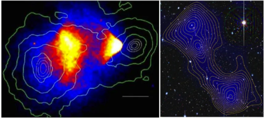
Figure 1.3 Left) Deep Chandra image of the Bullet cluster. Green lines represent mass contours from weak lensing. Right) Dark filament in the system Abell 222/223, reconstructed using weak lensing.

tive of the existence of large amounts of missing mass, which can be attributed to a DM component.

Modern determinations through weak lensing techniques provide a better gravitational determination of the cluster masses [10, 7] (see Fig. 1.2). I recommend reading through Ref.[9] for a derivation of the virial theorem in the context of Galaxy clusters.

Dynamical systems. The Bullet Cluster (1E 0657-558) is a paradigmatic example of the effect of dark matter in dynamical systems. It consists of two galaxy clusters which underwent a collision. The visible components of the cluster, observed by the Chandra X- ray satellite, display a characteristic shock wave (which gives name to the whole system).

On the other hand, weak-lensing analyses, which make use of data from the Hubble Space Telescope, have revealed that most of the mass of the system is displaced from the visible components. The accepted interpretation is that the dark matter components of the clusters have crossed without interacting significantly (see e.g., Ref. [11, 12]).

The Bullet Cluster is considered one of the best arguments against MOND theories (since the gravitational effects occur where there is no visible matter). It also sets an upper bound on the self-interaction strength of dark matter particles.

DM filaments. Observations of the distribution of luminous matter at large scales have shown that it follows a filamentary structure. Numerical simulations of structure formation with cold DM have been able to reproduce this feature. To date, it is well understood that DM plays a fundamental role in creating that filamentary network, gravitationally trapping the luminous matter. Recently, the comparison of the distribution of luminous matter in the Abell 222/223 supercluster with weak-lensing data has shown the existence of a dark filament joining the two clusters of the system. That filament, having no visible counterpart, is believed to be made of DM.

1.1.3 Cosmological scale

Finally, DM has also left its footprint in the anisotropies of the Cosmic Microwave Back- ground (CMB). The analysis of the CMB constitutes a primary tool to determine the cosmological parameters of the Universe. The data obtained by dedicated satellites in the past

(11)

DARK MATTER PROPERTIES 5

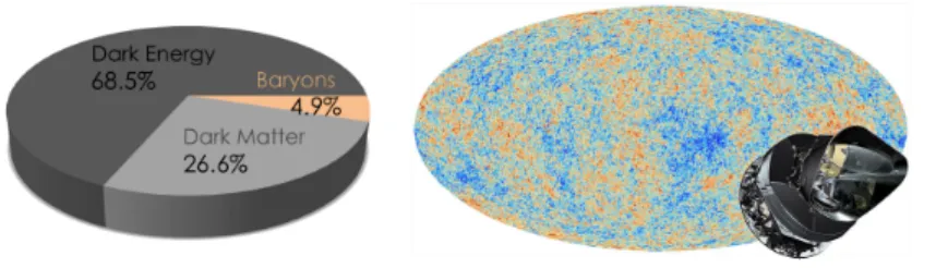
Figure 1.4 Left) Contribution to the energy density for each of the components of the Universe.

Right) Planck temperature map.

decades has confirmed that we live in a flat Universe (COBE), dominated by dark matter and dark energy (WMAP), whose cosmological abundances have been determined with great precision (Planck).

The abundance of DM is normally expressed in terms of the cosmological density parameter, defined asΩDMh² = ρDM/ρc whereρc is the critical density necessary to re- cover a flat Universe andh= 0.7is the normalised Hubble parameter. The most recent measurements by the Planck satellite, combined with data obtained from Supernovae (that trace the Universe expansion) yield

Ω_CDMh²= 0.1196±0.0031. (1.2) Given thatΩ≈1, this means that dark matter is responsible for approximately a 26% of the Universe energy density nowadays. Even more surprising is the fact that another exotic component is needed, dark energy, which makes up approximately the 69% of the total energy density (see Fig. 1.4).

1.2 Dark Matter properties 1.2.1 NonBaryonic

The results of the CMB, together with the predictions from Big Bang nucleosynthesis, suggest that only4−5%of the total energy budget of the universe is made out of ordinary (baryonic) matter. Given the mismatch of this with the total matter content, we must conclude that DM is non-baryonic.

Neutrinos. Neutrinos deserve special mention in this section, being the only viable non- baryonic DM candidate within the SM. Neutrinos are very abundant particles in the Uni- verse and they are known to have a (very small) mass. Given that they also interact very feebly with ordinary matter (only through the electroweak force) they are in fact a component of the DM. There are, however various arguments that show that they contribute in fact to a very small part.

First, neutrinos aretoo light. Through the study of the decoupling of neutrinos in the early universe we can compute their thermal relic abundance. Since neutrinos are relativistic particles at the time of decoupling, this is in fact a very easy computation (we will come back to this in Section 2.2.1), and yields

Ωνh²≈ P

im_i

91 eV . (1.3)

(12)

Using current upper bounds on the neutrino mass, we obtain Ωνh² < 0.003, a small fraction of the total DM abundance.

Second, neutrinos arerelativistic (hot) at the epoch of structure formation. As mentioned above, hot DM leads to a different hierarchy of structure formation at large scales, with large objects forming first and small ones occurring only after fragmentation. This is inconsistent with observations.

1.2.2 Neutral

It is generally argued that DM particles must be electrically neutral. Otherwise they would scatter light and thus not be dark. Similarly, constrains on charged DM particles can be extracted from unsuccessful searches for exotic atoms. Constraints on heavy millicharged particles are inferred from cosmological and astrophysical observations as well as direct laboratory tests [13, 14, 15]. Millicharged DM particles scatter off electrons and protons at the recombination epoch via Rutherford-like interactions. If millicharged particles cou- ple tightly to the baryonphoton plasma during the recombination epoch, they behave like baryons thus affecting the CMB power spectrum in several ways [13, 14]. For particles much heavier than the proton, this results in an upper bound of its charge[14]

≤2.24×10⁻⁴(M/1 TeV)^1/2. (1.4) Similarly, direct detection places upper bounds on the charge of the DM particle [16]

≤7.6×10⁻⁴(M/1 TeV)^1/2. (1.5) 1.2.3 Nonrelativistic

Numerical simulations of structure formation in the Early Universe have become a very useful tool to understand some of the properties of dark matter. In particular, it was soon found that dark matter has to be non-relativistic (cold) at the epoch of structure formation. Relativistic (hot) dark matter has a larger free-streaming length (the average distance traveled by a dark matter particle before it falls into a potential well). This leads to incon- sistencies with observations.

However, at the Galactic scale, cold dark matter simulations lead to the occurrence of too much substructure in dark matter haloes. Apparently this could lead to a large number of subhaloes (observable through the luminous matter that falls into their potential wells).

It was argued that if dark matter waswarm(having a mass of approximately2−3keV) this problem would be alleviated.

Modern simulations, where the effect of baryons is included, are fundamental in order to fully understand structure formation in our Galaxy and determine whether dark matter is cold or warm.

1.2.4 Long-lived

Possibly the most obvious observation is that DM is a long-lived (if not stable) particle.

The footprint of DM can be observed in the CMB anisotropies, its presence is essential for structure formation and we can feel its gravitational effects in clusters of galaxies and galaxies nowadays.

Stable DM candidates are common in models in which a new discrete symmetry is imposed by ensuring that the DM particle is the lightest with an exotic charge (and there-

(13)

DARK MATTER PROPERTIES 7

fore its decay is forbidden). This is the case, e.g., in Supersymmetry (when R-parity is imposed), Kaluza-Klein scenarios (K-parity) or little Higgs models.

However, stability is not required by observation. DM particles can decay, as long as their lifetime is longer than the age of the universe. Long-livedDM particles feature very small couplings. Characteristic examples are gravitinos (whose decay channels are gravitationally suppressed) or axinos (which decays through the axion coupling).

1.2.5 Collisionless

Dynamical systems, such as cluster collisions, set an upper bound to the self-interactions of DM particles. Observations seem to suggest that the DM component in these objects is mostly collision-less, thus behaving very differently than ordinary matter. Dark matter’s lack of deceleration in the bullet cluster constrains its self-interaction cross-sectionσ/m <

1.25cm²g⁻¹≈2barn GeV⁻¹.

Notice however, that self-interacting dark matter with a cross section in the range0.1<

σ/m <1cm²g⁻¹can be very beneficial in order to alleviate the problems with the amount of substructure in numerical simulations of DM haloes.

[17]

(14)

(15)

CHAPTER 2 FREEZE OUT OF MASSIVE SPECIES

In this chapter we will address the computation of the relic abundance of dark matter particles, making special emphasis in the case of thermal production in the Early Universe.

2.1 Cosmological Preliminaries

This section does not intend to be a comprehensive review on Cosmology, but only an introduction to some of the elements that we will need for the calculation of Dark Matter freeze-out.

We can describe our isotropic and homogeneous Universe in terms of the Friedman- Lemaˆıtre-Robertson-Walker (FLRW) metric, which is exact solution of Einstein’s field equations of general relativity

ds²=dt²−a²(t) dr²

1−kr² +r²(dθ²+ sinθdφ²)

=gµνdx^µdx^ν. (2.1) The constantk = {−1,0,+1}corresponds to the spatial curvature, with k = 0corre- sponding to a flat Universe (the choice we will be making in these notes). The affine connection, used to connect nearby tangent spaces (thus enabling the differentiation of tangent vector fields), is defined as

Γ^µ_νλ= 1

2g^µσ(gσν,λ+gσλ,ν−gνλ,σ), (2.2)

Dark Stuff.

9

(16)

10 FREEZE OUT OF MASSIVE SPECIES

These can also be found in the literature as Christoffel symbols, used in the definition of a covariant derivative. They are greatly simplified in the case of a FLRW metric, since most of the derivatives vanish.

The expansion of the Universe is controlled by the scale parametera(t). More specif- ically, we can define the Hubble parameter,H ≡ a(t)/a(t)˙ (where the dot denotes time derivation), which encodes the rate at which space is expanding. In the following, we are going to work with a radiation-dominated Universe. Notice that matter-radiation equality only occurs very late (when the Universe is approximately 60 kyr) and dark matter freeze- out occurs before BBN. The Hubble parameter for a radiation-dominated Universe reads

H = 1.66g^1/2_∗ T² MP

, (2.3)

whereMP = 1.22×10¹⁹GeV.

It is customary to define the dimensionless parameterx=m/T (wheremis a mass parameter that we will later associate to the DM mass) and extract the explicitxdependence from the Hubble parameter to defineH(m)as follows

H(m) = 1.66g^1/2_∗ m² MP

=Hx². (2.4)

In this section we will try to compute the time evolution of the number density of dark matter particles, in order to be able to compute their relic abundance today and what this implies in the interaction strength of dark matter particles. The phase space distribution functionf describes the occupancy number in phase space for a given particle inkinetic equilibrium, and distinguishes between fermions and bosons.

f = 1

e^(E−µ)/T ±1 , (2.5)

where the(−)sign corresponds to bosons and the(+)sign to fermions. Eis the energy andµthe chemical potential. For species in chemical equilibrium, the chemical potential is conserved in the interactions. Thus, for processes such as i+j ↔ c+dwe have µ_i+µ_j=µ_c+µ_d. Notice then that all chemical potentials can be expressed in terms of the chemical potentials of conserved quantities, such as the baryon chemical potentialµ_B. The number of independent chemical potentials corresponds to conserved particle numbers.

This implies, for example, that given a particle withµ_i, the corresponding antiparticle would have the opposite chemical potential−µi. For the same reason, since the number of photons is not conserved in interactions,µγ = 0

Using the expression of the phase space distribution function (2.5), and integrating in phase space, we can compute a series of observables in the Universe. In particular, the number density of particles,n, the energy density, ρ, and pressure, p, for a dilute and weakly-interacting gas of particles with g internal degrees of freedom read

n = g

(2π)³ Z

f(p)d³p, (2.6)

ρ = g

(2π)³ Z

E(p)f(p)d³p, (2.7)

p = g

(2π)³

Z |p|²

3E(p)f(p)d³p. (2.8)

(17)

COSMOLOGICAL PRELIMINARIES 11

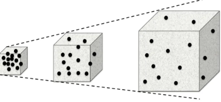
Figure 2.1 In the absence of number changing processes, the comoving number density of a species is preserved.

It is customary (and very convenient) to define densities normalised by the time dependent volumeV(t) =a(t)³. The reason for this is that in the absence of number changing processes, the comoving number density remains constant with time evolution (or red- shift) as exemplified in Fig. 2.1. An expanding Universe is a closed system and in thermal equilibrium the total entropy is conserved.

T dS=d(ρV) +pdV =d((ρ+p)V)−V dp= 0, (2.9) where we have used thatd((ρ+p)V) = V dp. The entropy density is therefores = S/V = (ρ+p)/V. Notice that since the evolution of the Universe is isoentropic, the entropy densitys=S/a³has precisely that dependence. Applying this prescription to the number density of particles, we define the yield as a fraction of the number density and the entropy density as

Y =n

s . (2.10)

Notice that, in the absence of number-changing processes, the yield remains constant.

The evolution of the entropy density as a function of the temperature is given by¹ s=2π²

45 g_∗sT³, (2.11)

where the effective number of relativistic degrees of freedom for entropy is g_∗s= X

bosons

g Ti

T ³

+7 8

X

fermions

g Ti

T ³

. (2.12)

Remember also that we can express the energy density as ρ= π²

30g_∗T⁴, (2.13)

in terms of the relativistic number of degrees of freedom g_∗= X

bosons

g Ti

T ⁴

+7 8

X

fermions

g Ti

T ⁴

. (2.14)

1To arrive at this equation, one can calculates= (p+ρ)/Tfor fermions and bosons, using the corresponding expression for the phase space distribution function.

(18)

In these two equations,T is the temperature of the plasma (in equilibrium) andTi is the effective temperature of each species.

Solving the integral in eq. (2.6) explicitly for relativistic and non-relativistic particles, and expressing the results in terms of the Yield results in the following expressions.

relativistic species

n= gef f

π² ζ(3)T³, (2.15)

wheregef f =gfor bosons andgef f = ³₄gfor fermions². Then, using eq. (2.10), the Yield at equilibrium reads

Y_eq= 45

2π⁴ζ(3)g_{ef f} g∗s

≈0.278g_{ef f} g∗s

. (2.16)

non-relativistic species

n=g mT

2π ^3/2

e^−m/T . (2.17)

Then the Yield at equilibrium reads Yeq = 45

2π⁴ π

8 1/2 g

g_∗s m

T 3/2

e^−m/T. (2.18)

EXAMPLE 2.1

It is easy to estimate the value of the Yield that we need in order to reproduce the correct DM relic abundance,Ωh²≈0.1, since

Ωh²=ρχ

ρ_ch²=mχnχh²

ρ_c = mχY_∞s0h²

ρ_c , (2.19)

whereY_∞ corresponds to the DM Yield today ands0is todays entropy density. We can assume that the Yield did not change since DM freeze-out and therefore

Ωh²=mχYfs0h² ρc

. (2.20)

Using the measured values0= 2970cm⁻³, and the value of the critical densityρc= 1.054×10⁻⁵h² GeV cm⁻³, as well as Planck’s result on the DM relic abundance, Ωh²≈0.1, we arrive at

Yf ≈3.55×10⁻¹⁰

1 GeV mχ

. (2.21)

In Figure 2.2 represent the yield as a function ofxfor non-relativistic particles, using expression(2.18). As we can observe, the above range of viable values forYf correspond toxf ≈ 20. Notice that this is a crude approximation and we will soon be making a more careful quantitative treatment.

2We are using here the approximationE≈ |~p|in the relativistic limit, and the integralsR∞

0 p²/(e^p−1)dp= 2ζ(3), andR∞

0 p²/(e^p+ 1)dp= 3ζ(3)/2, in terms or Riemann’s Zeta function. Remember also thatζ(3)≈ 1.202.

(19)

TIME EVOLUTION OF THE NUMBER DENSITY 13

Figure 2.2 Equilibrium yield as a function of the dimensionless variable,x, for non-relativistic particles. The green band represents the freeze-out value,Yf, for which the correct thermal relic abundance is achieved (for masses of order 1-1000 GeV.

2.2 Time evolution of the number density

The evolution of the number density operator can be computed by applying the covariant form of Liuvilles operator to the corresponding phase space distribution function. Formally speaking, we have

L[fˆ ] =C[f], (2.22)

whereLˆis the Liouville operator, defined as Lˆ =p^µ ∂

∂x^µ −Γ^µ_σρp^σp^ρ ∂

∂p^µ, (2.23)

andC[f]is the collisional operator, which takes into account processes which change the number of particles (e.g., annihilations or decays). In this expression, we have used the geodesic equationdp^µ/dτ =d²x^µ/dτ² = −Γ^µ_ρσdx^σ/dτ dx^ρ/dτ = −Γ^µ_ρσp^σp^ρ. In the expression above, gravity enters through the affine connection,Γ^µ_σρ.

One can show that in the case of a FRW Universe, for whichf(x^µ, p^µ) =f(t, E), we have

Lˆ = E∂

∂t −Γ⁰_σρp^σp^ρ ∂

∂E

= E∂

∂t −H|p|² ∂

∂E . (2.24)

(20)

Integrating over the phase space we can relate this to the time evolution of the number density

g (2π)³

Z L[fˆ ]

E d³p= g (2π)³

Z C[f]

E d³p, (2.25)

The integral on the left-hand side can be easily done by parts, which results in dn

dt + 3Hn = g (2π)³

Z C[f]

E d³p, (2.26)

Regarding the collisional operator, it encodes the microphysical description in terms of Particle Physics, and incorporates all number-changing processes that create or deplete particles in the thermal bath. For simplicity, let us concentrate in annihilation processes, where SM particles(A, B)can annihilate to form a pair of DM particles (labelled 1, 2), or vice-versa(A, B↔1,2). The phase space corresponding to each particle is defined as

dΠi= gi

(2π)³ d³pi

2E_i , (2.27)

from where g (2π)³

Z C[f]

E d³p = − Z

dΠAdΠBdΠ1dΠ2(2π)⁴δ(pA+pB−p1−p2)

|M_12→AB|²f1f2(1±fA)(1±fB)

−|M_AB→12|²fAfB(1±f1)(a±f2)

= −

Z

dΠ_AdΠ_BdΠ₁dΠ₂(2π)⁴δ(p_A+p_B−p₁−p₂) |M_12→AB|²f₁f₂− |M_AB→12|²f_Af_B

. (2.28)

The terms(1±fi)account for the viable phase space of the produced particles, taking into account whether they are fermions(−)or bosons (+). Assuming no CP violation in the DM sector (T invariance)|M12→AB|² = |MAB→12|² ≡ |M|². Also, energy conservation in the annihilation process allows us to writeE_A+E_B=E₁+E₂, thus,

fAfB=f_Aêqf_Bêq =e⁻ÊA⁺^TÊB =e⁻Ê^{1 +}^TÊ¹ =f₁êqf₂êq. (2.29) In the first equality we have just used the fact that SM particles are in equilibrium. This eventually leads to

g (2π)³

Z C[f]

E d³p=−hσvi n²−n²_eq

, (2.30)

where we have defined thethermally-averagedcross-section as hσvi ≡ 1

n²_eq Z

dΠAdΠBdΠ1dΠ2(2π)⁴δ(pA+pB−p1−p2)|M|²f₁^eqf₂^eq. (2.31) Collider enthusiasts would realise that this expression is similar to that of a cross-section, but we have to consider that the “initial conditions” do not correspond to a well-defined energy, but rather we have to integrate to the possible energies that the particles in the thermal bath may have. This explains the extra integrals in the phase space of incident

(21)

particles with a distribution function given byf₁^eqf₂^eq. We are thus left with the familiar form of Boltzmann equation,

dn

dt + 3Hn=−hσvi n²−n²_eq

. (2.32)

Notice that this is an equilibrium-restoring equation. If the right-hand-side of the equation dominates, thenntraces its equilibrium valuen ≈n_eq. However, whenHn > hσvin², then the right-hand-side can be neglected and the resulting differential equationdn/n =

−3da/a implies thatn ∝ a⁻³. This is equivalent to saying that DM particles do not annihilate anymore and their number density decreases only because the scale factor of the Universe increases.

It is also customary to define the dimensionless variable³ x=m

T . (2.33)

EXAMPLE 2.2

Using the yield defined in equation (2.10) we can simplify Boltzmann equation. No- tice that

dY dt = d

dt n

s = d

dt a³n

a³s

= 1 a³s

3a²an˙ +a³dn dt

= 1 s

3Hn+dn dt

. (2.34) Here we have used that the expansion of the Universe is iso-entropic and thusa³s remains constant. Also we use the definition of the Hubble parameterH = ^a_a^˙. This allows us to rewrite Boltzmann equation as follows

dY

dt =−shσvi Y²−Y_eq²

. (2.35)

Now, sincea∝T⁻¹ands∝T³, d

dt(a³s) = 0→ d

dt(aT) = 0→ d dt

a x

= 0, (2.36)

which in turns leads to

dx

dt =Hx , (2.37)

and thus

dY dt =dY

dx dx

dt =dY

dx Hx . (2.38)

Using the results of Example (2.2) we can express Boltzmann equation (2.32) as dY

dx = −sxhσvi

H(m) Y²−Y_eq²

= −λhσvi

x² Y²−Y_eq²

, (2.39)

3It is important to point that this definition ofxis not universal; some authors useT /mand care should be taken when comparing results from different sources in the literature.

(22)

where we have used the expression of the entropy density (2.11) in the last line and defined λ ≡ 2π²

45

MPg_∗s 1.66g_∗^1/2

m

≈ 0.26 g_∗s g_∗^1/2

M_Pm . (2.40)

Eq. (2.39) is a Riccati equation, without closed analytical form. Thus, to calculate its solutions we have to rely on numerical methods. However, it is possible to solve it approximately.

2.2.1 Freeze out of relativistic species

The freeze-out of relativistic species is easy to compute, since the yield (2.16) has no dependence onxf. Neutrinos are a paradigmatic example of relativistic particles and one must in principle consider their contribution to the total amount of dark matter (after all, they are dark).

Since neutrinos decouple while they are still relativistic, their yield reads Yeq ≈0.278gef f

g_∗s . (2.41)

Neutrinos decouple at a few MeV, when the species that were still relativistic aree^±,γ,ν and¯ν. Thus, the number of relativistic degrees of freedom isg_∗ =g_∗s= 10.75. For one neutrino family, the effective number of degrees of freedom isg_{ef f} = 3g/4 = 3/2. Using these values, the relic density today an be written as

Ωh² = P

imν_iY_∞s0h² ρc

≈ P

imν_i

91 eV . (2.42)

Notice that in order for neutrinos to be the bulk of dark matter, we would needP

imν_i ≈ 9 eV, which is much bigger than current upper limits (for example, obtained from cosmological observations). Notice, indeed, that if we consider the current boundP

imν_i ≤ 0.3 eVwe can quantify the contribution of neutrinos to the total amount of dark matter, resulting inΩh²≤0.003. This is less than a 3% of the total dark matter density.

2.2.2 Freeze out of non-relativistic species

The case of non-relativistic species is far more interesting. Once We can define the quantity

∆Y ≡Y −Yeq. (2.43)

Boltzmann equation (2.39) is now easier to solve, at least approximately, as follows For early times,1 < x xf, the yield follows closely its equilibrium value,Y ≈ Yeq, and we can assume thatd∆Y/dx= 0. We then find

∆_Y =−

dYeq

dx

Yeq

x²

2λhσvi. (2.44)

(23)

Thus, at freeze-out we obtain

∆Y_f ≈ x²_f

2λhσvi, (2.45)

where in the last line we have used that for large enoughx, using eq. (2.18) implies

dY_eq

dx ≈ −Yeq.

For late times,xx_f, we can assume thatY Y_eq, and thus∆_Y_∞ ≈Y_∞, leading to the following expression,

d∆Y

dx ≈ −λhσvi

x² ∆²_Y , (2.46)

This is a separable equation that we integrate from the freeze-out time up to nowadays. In doing so, it is customary to expand the thermally averaged annihilation cross section in powers ofx⁻¹ashσvi=a+^b_x.

Z ∆_Y∞

∆_Yf

d∆Y

∆²_Y =− Z x∞

xf

λhσvi

x² dx . (2.47)

Taking into account thatx_∞x_f, this leads to 1

∆Y∞

= 1

∆Y_f

+ λ xf

a+ b

2xf

. (2.48)

The term1/∆Y_f is generally ignored (if we are only aiming at a precision up to a few per cent [18]) . We can check that this is a good approximation using the previously derived (2.45) forx_f ≈20(which, as we saw in Fig. 2.2 is the value for which the equilibrium Yield has the right value). This leads to

∆_Y_∞ =Y_∞= x_f λ

a+_2x^b

f

. (2.49)

The relic density can now be expressed in terms of this result as follows Ωh² = mχY_∞s0h²

ρc

≈ 10⁻¹⁰GeV⁻² a+₄₀^b

≈ 3×10⁻²⁷cm³s⁻¹

a+₄₀^b . (2.50)

This expression explicitly shows that for larger values of the annihilation cross section, smaller values of the relic density are obtained.

2.2.3 WIMPs

Equation (2.50) implies that in order to reproduce the correct relic abundance, dark matter particles must have a thermally averaged annihilation cross section (from now on we will

(24)

shorten this to simply annihilation cross section when referring tohσvi) of the order of hσvi ≈3×10⁻²⁶cm³s⁻¹.

We can now consider a simple case in which dark matter particles self-annihilate into Standard Model ones through the exchange (e.g., in an s-channel) of a gauge boson. It is easy to see that if the annihilation cross section is of orderhσvi ∼ G²_Fm²_{W IM P}, where GF = 1.16×10⁻⁵GeV⁻², then the correct relic density is obtained for masses of the order of∼GeV.

2.3 Computing the DM annihilation cross section

In the previous sections we have derived a relation between the thermally averaged annihilation cross section and the corresponding dark matter relic abundance. This is very useful, since it provides an explicit link with particle physics. A central point in that calculation was the expansion in velocities of the thermally averaged annihilation cross section.

hσvi=ha+bv²+cv⁴+. . .i=a+3 2

b⁰ x +15

8 c

x² +. . . . (2.51) Notice that in the expressions of the previous section we have definedb ≡3b⁰/2. As we also mentioned before, DM candidates tend to decouple whenxf ≈20. For this value, the rms velocity of the particles is about c/4, thus corrections of orderx⁻¹can in general not be ignored (they can be of order5−10%). Moreover, some selection rules can actually lead toa = 0 for some particular annihilation channels and in that casehσviis purely velocity-dependent.

It is important to define correctly the relative velocity that enters the above equation. In Ref. [18] an explicitly Lorentz-invariant formalism is introduced where

g1

Z

C[f1] d³p1

2π³E1

=− Z

hσviMøl(dn1dn2−dn^eq₁ dn^eq₂ ), (2.52) wherehσviMøln1n2is invariant under Lorentz transformations and equalsvlabn1,labn2,lab

in the rest frame of one of the incoming particles. In our case the densities and Møller velocity refer to the cosmic comoving frame. In terms of the particle velocities~v_i=~p_i/E_i,

v_Møl=

|~v₁−~v₂|²+|~v₁×~v₂|²^1/2

. (2.53)

The thermally-averaged product of the dark matter pair-annihilation cross section and their relative velocityhσvMøliis most properly defined in terms of separate thermal baths for both annihilating particles [18, 19],

hσvMøli(T) =

Rd³p₁d³p₂σv_Møle^−E¹^/Te^−E²^/T

Rd³p₁d³p₂e^−E¹^/Te^−E²^/T , (2.54) wherep1= (E1,p1)andp2= (E2,p2)are the 4-momenta of the two colliding particles, and T is the temperature of the bath. The above expression can be reduced to a one- dimensional integral which can be written in a Lorentz-invariant form as [18]

hσvMøli(T) = 1

8m⁴_χT K₂²(mχ/T) Z ∞

4m²_χ

ds σ(s)(s−4m²_χ)√ sK1

√ s T

, (2.55)

(25)

COMPUTING THE DM ANNIHILATION CROSS SECTION 19

wheres= (p1+p2)²andKidenote the modified Bessel function of orderi. In computing the relic abundance [20] one first evaluates eq. (2.55) and then uses this to solve the Boltzmann equation. The freeze out temperature can be computed by solving iteratively the equation

xf = ln mχ

2π³ r 45

2g_∗GN

hσvMøli(xf)x^−1/2_f

(2.56) whereg∗represents the effective number of degrees of freedom at freeze-out (√

g∗ ≈9).

As explained in the previous section, one finds that the freeze-out pointxf ≡mχ/Tf is approximatelyxf ∼20.

The procedure can be simplified if we consider that the annihilation cross section can be expanded in plane waves. For example, consider the dark matter annihilation process χχ → ij and assume that the thermally averaged annihilation cross section can be expressed ashσvi_ij ≈a_ij+b_ijx. It can then be shown that the coefficientsa_ijandb_ij can be computed from the corresponding matrix element. For example,

aij = 1 m²_χ

Nc

32πβ(s, mi, mj)1 2

Z 1

−1

dcosθCM|M_χχ→ij|²

s=4m²_χ

, (2.57)

whereθ_CMdenotes the scattering angle in the CM frame,N c= 3forqq¯ final states and 1 otherwise, and

β(s, mi, mj) =

1−(mi+mj)² s

^1/2

1−(mi−mj)² s

^1/2

(2.58) The contribution for each final state is calculated separately.

2.3.1 Special cases

The derivation of equation (2.50) relied on the expansion ofhσviin terms of plane waves.

This expansion can be done whenhσvivaries slowly with the energy (we can express this in terms of the centre of mass energys). However, there are some special cases in which this does not happen and which deserve further attention.

Annihilation thresholds

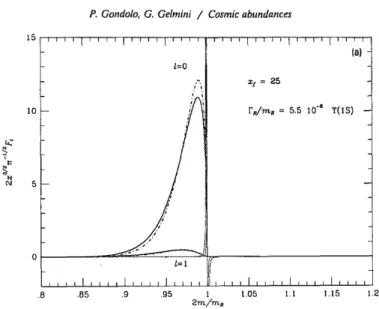
A new annihilation channelχ+χ→A+Bopens up when2mχ ≈mA+mB. In this case the expansion in velocities ofhσvidiverges (at the threshold energy) and it is no longer a good approximation [18]. Notice in particular that below the threshold, the expression ofaij in Equation (2.57) is equal to zero (as it is only evaluated for s >4m²_χ). A qualitative way of understanding this is of course that DM particles have a small velocity, which is here approximated to zero. In the limit of zero velocity, the total energy available is determined by the DM mass.

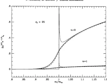
However, we are here ignoring that a fraction of DM particles (given by their thermal distribution in the Early Universe) have a kinetic energy sufficient to annihilate into heavier particles (above the threshold). In other words,hσviis different from zero below the corresponding thresholds. A very good illustration of this effect is shown in Ref. [18] and is here reproduced in Fig. 2.3.

The thin solid line corresponds to the approximate expansion in velocities and shows that not onlyhσviis zero below the threshold, but also diverges at the threshold,

(26)

Figure 2.3 Relativistic thermal average near a threshold (thick solid line) compared to the result fro the expansion in powers ofx⁻¹(thin line). Figure from Ref. [18].

thereby not leading to a good solution. Expression (2.55), represented by a thick solid line, still provides a good solution .

Resonances

The annihilation cross section is not a smooth function of s in the vicinity of an s- channel resonance. Thus, the velocity expansion of hσvi will fail (although once more, expression (2.55) still provides a good solution). For a Breit-Wigner resonance (due to a particleφ) we have

σ= 4πw

p² B_iB_f m²_φΓ²_φ

(s−m²_φ)²+m²_φΓ²_φ, (2.59) in terms of the centre of mass momentump= 1/2(s−4m²)^1/2and the statistical factorw = (2J + 1)/(2S+ 1)². The quantitiesBi,f correspond to the branching fractions of the resonance into the initial and final channel.

We can define the kinetic energy per unit mass in the lab frame,, as =(E1,lab−m) + (E2,lab−m)

2m = 2−4m²

4m² , (2.60)

and rewrite the expression forσ in the lab frame (we want to use Equation (3.21) in Ref. [18] to compute hσvMøli). Summing to all final states, and using vlab = 2^1/2(1 +)^1/2/(1 + 2), we obtain

σvlab=8πw

m² bφ() γ²_φ

(−²_φ)²+γ_φ² , (2.61) with the definitionsb() =Bi(1−Bi)(1 +)^1/2/(^1/2(1 + 2),γφ =mφΓφ/4m², andφ= (m²_φ−4m²)/4m².

(27)

COMPUTING THE DM ANNIHILATION CROSS SECTION 21

Figure 2.4 Relativistic thermal average in a resonance (thick solid line) compared to the result fro the expansion in powers ofx⁻¹(thin line). Figure from Ref. [18].

It can be shown that in the case of a very narrow resonance,γ_φ 1, the expression above can be approximated as

σv_lab=8πw

m² b_φ()πγ_φδ(−_φ), (2.62) the relativistic formula for the thermal average then reads [18]

hσv_Møli= 16πw m²

x

K₂²(x)πγ_φ^1/2_φ (1 + 2e_φ)K₁(2xp

1 +_φ)b_φ(e_φ)θ(_φ). (2.63) Notice thatφ > 0whenm < 2mφ, i.e., when the mass of the DM is not enough to enter the resonance. The reason is easy to understand. Only through the extra kinetic energy provided by the thermal bath, the resonance condition can be satisfied.

However, when the mass of the DM exceeds the resonance condition, the kinetic energy only takes us further away from the resonant condition and the thermalised cross section tends to vanish. In other words, the centre of mass rest energy exceeds m_φ/2. This can be seen in Figure 2.4.

For a large width the expression has to be computed numerically and can be found in Ref. [18].

Coannihilations

When deriving Boltzmann equation (2.32) we have only considered one exotic species, but this needs not be the case. In fact, in most particle models for DM, there are more exotic species that we need to take into account. Notice that, in principle, this would lead to a system of coupled Boltzmann equations. If we label exotic species asχi, withi= 0, 1. . . k, and SM particles asA, B, we have to consider all number chang-

(28)

ing processes for each species,

(i) χi+χj→A+B (ii) χi+A→χj+B (iii) χj →χi+A

If we consider the (usual) case in which the DM is protected by a symmetry (e.g., in the case of Supersymmetric theories) and that the exotic particles all must decay eventually into the lightest oneχ0, then, we must only trace the evolution of the total number density of exotic species,n = Pk

i=0ni. Under this assumption, processes (ii) and (iii) do not need to be considered, as they do not change the number of exotics.

This is correct as long as the rate of these is faster than the expansion of the Universe.

Regarding process (i) we have to be aware that the cross sectionσijis going to appear multiplied by the corresponding number densities,ninj . Now, we are considering the case in which both particlesiandjare non-relativistic and as a consequence,ni,j

are Boltzmann suppressed,n_i,j/e^−m^i,j^/T . Thus, unlessm_j≈m_i, the abundance of χ_jis negligible and only the processχ_i+χ_j→A+Bis important (and we are back to the case of a single exotic).

However, whenm_j ≈m_i, there can be coannihilation effects and particlejmay serve as a channel through which particles i can be more effectively depleted. This is the case, e.g., of the stau and the neutralino in supersymmetric theories.

2.4 Freeze-in of dark matter

In the previous section, we have explained in full detail how DM particles can be produced in the early Universe through pair-annihilation processes. As we discussed earlier, if the annihilation cross section happens to be of the order to the Electroweak scale, the resulting relic density is of the right order to reproduce the observed DM abundance. However, this WIMP paradigm is by no means the only way in which DM particles can be produced in the right amount. In this section, we will address another interesting possibility that is applicable to particles with a much smaller interaction scale.

Let us begin by assuming that the DM particles,χ, has extremely weak interactions, and that its initial abundance is zero. An implicit assumption in all of this is that the reheating temperature of the Universe after inflation was not high enough forχ to be in thermal equilibrium. Notice that DM particles can still be produced by interactions of particles in the thermal bath (following the notation of Ref. [21], we will refer to bath particles asB_i).

The production rate is small, as a consequence of the small DM coupling, however, since they are produced out of equilibrium, these DM particles do not annihilate (and of course do not decay). As a consequence, a relic density builds up. The final DM density depends on the specific interactions with bath particles.

In order to carry out the computation, notice that we can make use of Boltzmann equation, as formulated in eq. (2.26), but now we have to write the collisional operator accord- ing to the interactions of DM particles with those of the bath. We will here consider one characteristic example, that should serve as a guide to consider other possibilities.

(29)

FREEZE-IN OF DARK MATTER 23

2.4.1 DM production from decays of heavier bath particles

Consider the decay of a heavy bath particle into a lighter one and a DM particle,B2 → B1χ. IfmB2 > mB1+mχ this process will dominate DM production. The collisional operator is easy to write,

dn

dt + 3Hn = g (2π)³

Z C[f] E d³p

= Z

dΠB1dΠB2dΠχ(2π)⁴δ⁴(pB2−pB1−pχ)×

h|MB2→B1χ|² fB2(1±fB1)(1±fχ)− |MB1χ→B2|² fB1fχ(1±fB2)i

= Z

dΠB2ΓB22gB2mB2fB2. (2.64)

In the last line we have assumed no Pauli blocking to approximate(1±fB1)≈1and we have neglected the initial abundance of DM particles,f_χ ≈ 0. We have also expressed

|MB2→B1χ|² in terms of the decay width, Γ_B2, the number of degrees of freedom ob B₂and its mass. If we write the phase space element explicitly, and we consider that for particles in thermal equilibrium we can approximatef_B₂ = 1/(e^E^B²^/T ±1)≈e^−E^B²^/T, we are left with

dn

dt + 3Hn = gB₂

Z ∞

m_B₂

d³pB2

(2π)³

fB2ΓB2mB2

EB₂

. (2.65)

The integral on the right-hand side is easy to solve, as it can be reduced to the first modified Bessel function of the second kind,K1(mB₂/T), resulting in

dn

dt + 3Hn = gB₂ΓB₂m²_B

2

2π² T K₁(m_B₂/T). (2.66) As we did in the previous section, it is much simpler to rewrite this expression in terms of the derivative of the yieldY =n/sin terms of the dimensionless variablex=m_B₂/T, which leads to

Y = 45g_B₂M_pΓ_B₂ 4π⁴(1.66)m²_B

2g^S_∗√ g_∗

Z ∞

x_min

K1(x)x³dx . (2.67) Finally, solving forxmin= 0, yields

Y ≈ 135g_B₂ 8π³(1.66)g^S_∗√

g_∗

Γ_B2M_p m²_B

2

. (2.68)

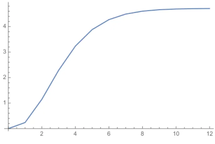
The functionK₁(x)x³has a maximum aroundx≈2.4and its integralRx_max

0 K₁(x)x³dx stabilises abovex_max≈8, we have plotted this behaviour in Fig. 2.5. As we can observe, the final yield is proportional to the bath’s particle partial decay width. This is very interesting, as the decay width is directly proportional to the DM coupling square. Thus, the final yield (and DM relic abundance) increases if the DM coupling increases. This behaviour is the opposite as observed for WIMPs in eq.(2.49). This behaviour holds as long as the DM coupling is small. If we increase the DM coupling, there comes a point at which the DM particles produced reach thermal equilibrium and then we have to go back to the freeze-out computation of the previous section.

(30)

2 4 6 8 10 12

1 2 3 4

Figure 2.5 Yield of a freeze-in species (in arbitrary units) as a function ofx=m/T.

Finally, from eq.(2.68) we can use the explicit expression for the partial decay width in a two-body final state and compute the resulting relic density. It can be seen that in order to reproduce the correct relic abundance, the coupling needed is of the order of λ≈10⁻¹³. Interestingly, the final value of the Yield is also sensitive to the initial value of x_minfrom which we integrate. Notice thatx_minwill be given by the temperature at which the Universe reheated after inflation. Thus, the frreeze-in mechanism has a very interesting connection to inflation.

A similar computation can be made for other possible production channels, for example, scattering of bath particlesB1B2→B3χ. In this case, the Boltzmann equation (2.64) has to be modified accordingly taking into account the matrix elements of the process and the number densities of the particles involved.

The freeze in mechanism has been used for example to argue that gravitinos (the supersymmetric companion of the graviton) and axinos (the supersymmetric companion of the axion) can be viable candidates for DM.

2.5 Late decays of unstable particles

As we have just seen in the freeze-in mechanism of the previous section, it is conceivable that particles with a small coupling to SM ones are produced out of equilibrium due to either scattering or decays of particles in the thermal bath. The frozen-in particles need not be absolutely stable, but given their small couplings their lifetime can be large. If the lifetime is larger than the age of the Universe (10¹⁷s), we should not worry as the computation of the relic density is not altered and this simply corresponds to a case of decaying DM (very interesting from the point of view of indirect detection). However, if the lifetime is smaller, then it is obvious that this particle cannot be the DM. Late-decaying particles can however contribute to the (non-thermal) production of DM. A possible scenario is as follows.

Consider a canonical WIMP DM candidate,χ1, which decoupled atx=mχ₁/T ≈20 via a freeze-out mechanism as described in Section 2.2.2, which leads to to athermal relic abundanceY_χ^th₁. Simultaneously, a semi-stable particleχ2, with very small couplings, freezes-in via the mechanism explained in Section 2.4, with a yieldYχ₂. If particleχ2

(31)

LATE DECAYS OF UNSTABLE PARTICLES 25

can decay into particleχ1(after the latter has frozen-out), then eventually all the number density of the heavy particle, is translated into the lighter one leading to anon-thermal contribution,Yχ₂ =Y_χ^nt₁. The total yield for the lighter particle is therefore the sum of both contributions

Yχ₁ =Y_χ^th₁ +Y_χ^nt₁. (2.69) This exotic scenario can occur in supersymmetric models, whereχ2 is the gravitino andχ1 is the lightest neutralino. It should be emphasized that the late decay of exotic particles (and the associated injection of electromagnetic and hadronic particles) can ruin the predictions of BBN and also alter the black body shape of the CMB spectrum. Stringent constraints exist if these decays occur after BBN, but in general the model is safe if the lifetime ofχ₂is smaller than approximately 1 minute.

(32)

(33)

CHAPTER 3 DIRECT DM DETECTION

3.1 Preliminaries 3.1.1 DM flux

We can easily estimate the flux of DM particles through the Earth. The DM typical velocity is of the order of300km s⁻¹∼10⁻³c. Also, the local DM density isρ0= 0.3GeV cm⁻³, thus, the DM number density isn=ρ/m.

φ=vρ m ≈10⁷

m cm⁻²s⁻¹ (3.1)

These particles interact very weakly with SM particles.

Assuming a typical WIMP cross sectionσ 3.1.2 Kinematics

Direct DM detection is based on the search of the scattering between DM particles and nuclei in a detector. This process is obly observable through the recoiling nucleus, with an energyE_R. DM particles move at non-relativistic speeds in the DM halo. Thus, the dynamics of their elastic scattering off nuclei are easily calculated. In particular, the recoiling energy of the nucleus is given by

E_R=1

2m_χv² 4m_χm_N (mχ+mN)²

1 + cosθ

2 (3.2)

Dark Stuff.

27