DETERMINING OPERATIONAL CAPITAL AT RISK:
AN EMPIRICAL APPLICATION TO THE RETAIL BANKING
ENRIQUE JOSÉ JIMÉNEZ- RODRÍGUEZ JOSÉ MANUEL FERIA-DOMÍNGUEZ
JOSÉ LUIS MARTÍN-MARÍN
FUNDACIÓN DE LAS CAJAS DE AHORROS DOCUMENTO DE TRABAJO
Nº 441/2009
De conformidad con la base quinta de la convocatoria del Programa de Estímulo a la Investigación, este trabajo ha sido sometido a eva- luación externa anónima de especialistas cualificados a fin de con- trastar su nivel técnico.
ISSN: 1988-8767
La serie DOCUMENTOS DE TRABAJO incluye avances y resultados de investigaciones dentro de los pro- gramas de la Fundación de las Cajas de Ahorros.
Las opiniones son responsabilidad de los autores.
DETERMINING OPERATIONAL CAPITAL AT RISK: AN EMPIRICAL APPLICATION TO THE RETAIL BANKING
ENRIQUE JOSÉ JIMÉNEZ- RODRÍGUEZ*
JOSÉ MANUEL FERIA-DOMÍNGUEZ**
JOSÉ LUIS MARTÍN-MARÍN***
Abstract
In this paper, we conduct an empirical application of the Advanced Measurement Approach (AMA), in particular the Loss Distribution Approach (LDA), to the Spanish retail banking sector for the estimation of Economic Capital for Operational Risk. Our results confirm that the implementation of such advanced approach in credit entities provides a lower consumption of regulatory capital, in comparison with the non-advanced methodologies, such us the Basic Indicator Approach (BIA) and the Standardised Approach (SA). At the same time, by focussing on the LDA model, we also assess the potential impact on the Capital at Risk (CaR) of the probability distribution parametric profile used when modelling the internal operational losses, recorded by the financial entity in its IOLD (Internal Operational Losses Database).
KEYWORDS: Operational Risk, Advanced Measurement Approach (AMA), Loss Distribution Approach (LDA), Capital at Risk (CaR), Internal Operational Losses Database (IOLD).
*Department of Business Administration - Pablo de Olavide University - Ctra. de Utrera, km. 1, 41013 (Seville, Spain), phone: +34954977925 fax: +34954348353 e-mail: [email protected]
** Department of Business Administration - Pablo de Olavide University - Ctra. de Utrera, km. 1, 41013 (Seville, Spain) phone: +34954349363 fax: +34954348353 e-mail: [email protected]
*** Department of Business Administration -Pablo de Olavide University - Ctra. de Utrera, km. 1, 41013 (Seville, Spain) -phone: +34954349056 fax: +34954348353 e-mail: [email protected]
1. INTRODUCTION.
In June 2004, the Basel Committee on Banking Supervision, henceforth the Committee, published the New Capital Accord, better known as Basel II. This regulatory framework is intended to enhance the security and solvency of the financial system, and is presented as a standard of capital adequacy that is more sensitive to the risk of banking operations. A key objective is to encourage financial entities to improve their own capacities for the management and control of risks. One of the principal novelties of Basel II is the inclusion of specific capital requirements to hedge operational risk; these are thus added to the requirements that the Basel I already establishes to cover both credit and market risk. In addition, the Committee (2004: 128) includes an explicit definition of operational risk since there had previously been no clear consensus on this concept. Specifically, operational risk is defined as follows:
“the risk of loss resulting from inadequate or failed internal processes, people and systems or from external events”.
The Basel Committee (2001) proposes three approaches for calculating the capital requirements to meet this risk; ranked from lower to higher degree of sophistication and sensitivity to the risk, these are: the Basic Indicator Approach (BIA), the Standardised Approach (SA) and the Advanced Measurement. Approach (AMA). In turn, within the AMA, three alternative methodologies are described: the Internal Measurement Approach (IMA), Scorecards, and the Loss Distribution Approach (LDA). This last, combined with the OpVaR (Operational Value at Risk) concept, appears to be the best-positioned methodology, in so far as it is more sensitive to this risk. The less advanced methodologies (Basic and Standardised approaches), are more conservative in estimating the regulatory capital required for operational risk, although they are easier to implement in practical terms. In these cases, ultimately, the capital required is calculated as a percentage of the Gross Income of the financial entity.
Starting from this premise, the main goal of this paper is to test, by means of an empirical application, whether the implementation of an advanced approach for the measurement of operational risk in credit entities provides a lower consumption of regulatory capital, in comparison with the less advanced methodologies. At the same time, considering in particular the LDA model, we assess the potential impact on the Capital at Risk (CaR) of the parametric profile of the probability distribution used when modelling the operational losses.
We begin the study by establishing the theoretical framework in which those methodologies of measurement proposed by the Committee have been conceived. Having defined this framework, the next step is to test of our main hypothesis. For this purpose, we have taken the historical information on operational losses provided by a Spanish credit entity, specialised in the retail banking sector. We thus devote the third part of this paper to the detailed analysis of the inputs employed, i.e. the data of
operational losses. Once the data are ready to be handled, and following the methodological sequence of the LDA approach, we have modelled the distributions of both frequency and severity, from which the distribution of aggregated losses is obtained. In this study, operational risk, within the retail banking sector, has been classified by event types. Thus we complete the analysis by computing the capital required for each of the 8 operational risk event types proposed by the Committee. Lastly, for the whole entity, we conduct a comparative analysis of the capital consumption depending on the measurement methodology used. The results of the study demonstrate a clear divergence between the capital estimated by applying the less advanced approaches and that provided by the LDA model, which resulted in a notable potential capital saving. In any case, it will be the responsibility of the national supervisor to validate the suitability of the internal measurement model proposed by the bank and, consequently, the resulting amount of regulatory capital required.
2. CONCEPTUAL FRAMEWORK.
The measurement of operational risk, in terms of regulatory capital, has become the most complex and, in turn, the most important aspect when addressing such a financial risk. The Committee (2001:
3) defines the Basic (BIA) and Standardised (SA) approaches as top-down methodologies. Both approaches determine the capital requirements for the global entity (in the BIA) or for each business line (in the SA). After this preliminary calculation, in a top down process, the assignment of capital is broken down by type of risk and by business unit or process, in particular. In contrast, the AMA approaches are based on so-called bottom-up methodologies; in these the capital required is calculated from internal loss data broken down by event type and by business line; after this specific calculation and following a process of working from the particular to the general, the capital requirement is computed, by aggregation, for the bank as a whole. To be allowed to apply the Standardised Method and the AMA methodologies, the banks must meet certain admission criteria (Basel, 2006: 148-155).
However, it is intended that the Basic Indicator Approach should be applicable to any bank, independently of the complexity of its activities, provided that it follows the directives of the document “Sound Practices for the Management and Supervision of Operational Risk” (Basel, 2002);
this Approach and the conditions included in the document thus constitute a departure point in the capital estimation process.
The Committee recommends that entities should adopt progressively more advanced approaches, from the range of methods available, as they develop more sophisticated systems and practices of measurement over time. Nevertheless, it should be stated that the development and implementation of more advanced techniques will, to a large extent, depend on the availability of internal data on operational losses. In this respect, the model that enjoys the widest acceptance in the banking industry is the Loss Distribution Approach (LDA), based on the concept of Operational Value at Risk (OpVaR) for the calculation of the capital charge.
=BIA K
n x GI
n
i
∑
n= =1
1 )
( K
...
BIA
α
( )
[ (
( ) ( )) ]
{
∑ 1 3 ∑ 1 8 1 8 0}
3= − max − − ,
KSA years GI xβ
2.1THE BASIC INDICATOR APPROACH (BIA).
Strictly speaking, the banks that apply the BIA approach must cover their operational risk with an amount of equity equivalent to a fixed percentage (denoted as alpha) of the average of their Gross Income (GI)1, annually for the last three financial years, as defined by the Committee (2004: 129). In the event of the GI for any year being zero or negative, that will not be taken into account when computing the average. The average would thus be determined as the sum of the positive annual figures divided by the number of positive annual figures (Basel, 2006: 159-160), calculated as follows:
(1) Where
KBIA: Capital requirement by the Basic Indicator Approach.
GI: Annual gross income.
α: The alpha coefficient, fixed in 15% by the Committee.
n: Number of years in which the GI has been positive, in the last three financial years.
2.2THE STANDARDISED METHOD (SA).
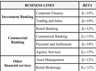
In the Standardised method (or Standardised Approach, SA) the activity of the bank is broken down into eight different business lines, defined by the Committee (2004: Annex 6). As in the BIA approach, the Gross Income of each line is taken as an indicator to reflect the operational risk exposure faced by the bank in this segment. For each business unit, the capital charge will be determined by the product of the Gross Income generated by a factor, termed beta, assigned to each of the lines. The total amount of capital required, at the level of the entity, will be obtained as the average of the last three years by summing up individual capital charges for each of the units described. Any negative capital requirements, resulting from negative gross income in any of the bank's business lines, can be used to off-set the positive requirements from other units, without any limit, as permitted by the Committee.
However, it affirms that, when the aggregate capital requirement calculated in any particular year is negative2, the numerator for that year will be zero. The analytical expression that summarises the indicator is the following:
(2)
1 It is intended that this measure, GI, should be net of interest, representing the spread between cost of funds and loan interest rates charged. Equally it should be gross of any provisions made; it should also exclude profits or losses made from the sale of securities from its investment portfolio; and should ignore extraordinary or exceptional items, and any income derived from insurance activities.
Where
KSA: Capital requirements by the Standardised Method.
GIi : Annual Gross Income by business line.
βi: Fixed percentage established by the Committee, which relates the amount of capital required to the gross income of each of the eight business lines (see table 1).
Table 1: Beta values for each business line.
BUSINESS LINES BETA
Corporate Finance β1=18%
Investment Banking
Trading and Sales β2=18%
Retail Banking β3=12%
Commercial Banking β 4=15%
Payment and Settlement β5=18%
Commercial Banking
Agency Services β 6=15%
Asset Management β7=12%
Other
financial services Retail Brokerage β 8=12%
Source: Basel Committee on Banking Supervision.
2.3.THE LOSS DISTRIBUTION APPROACH (LDA).
The Loss Distribution Approach is a statistical technique, inherited from the actuarial field (see Bühlmann, 1970), the objective of which is to obtain a probability distribution of aggregate losses. The model is based on the information of historical losses, recorded in the form of a matrix comprised by the eight business lines and the seven types of operational risk standardised by the Committee. When an operational loss is identified, it is essential to define two variables: first, the severity, or monetary amount of the loss; and, second, the frequency with which the event is repeated during a specified period of time, generally one year, or, put another way, the probability of that event occurs.
According to Böcker and Klüppelberg (2005), the severity is defined, from a statistical perspective, as:
"a continuous random variable,
( )
Xk k∈Ν, that takes positive values3, which are independent of each other, and identically distributed”. On the basis of this meaning, Panjer (2006: Chapter 4) establishes a compendium of the functions that, potentially, could be used for modelling it. However, in practice,
2 If the negative gross income of any year distorts the capital requirements, the supervisors will consider taking the appropriate supervisory actions under Pillar II.
3 As an accounting expense, the operational losses represent negative items in the profit and loss account of the entity;
however, in the modelling they are taken as positive values.
∑
==
(, )( , ) )
, (
j i N
n
n
i j L j
i S
0
the peculiar form of the distribution of operational losses4 means that the number of functions with significant fits is restricted. On this point, it must be stated that the principal difficulty when modelling the operational risk is the extreme behaviour of the severity distribution tails, which leads to Pareto probabilistic models, when high thresholds of losses are applied (Fontnouvelle et al., 2004).
Concerning the frequency, and following Frachot et al. (2003), the Poisson distribution is used successfully in the actuarial techniques, and is a suitable candidate since it is characterised by a single parameter (λ), which represents the number of events per year. However, authors like Da Costa (2004) suggest another useful rule to follow: choosing the Binomial model when the variance is less than the arithmetic mean (sub-dispersion), the Poisson model when both values are similar (equi-dispersion) and the Negative Binomial model when the variance is greater than the mean (over-dispersion). Once the distributions of severity and frequency have been characterised, we can proceed to obtain the aggregate loss distribution, S(i,j), using an actuarial technique termed convolution5. Thus, the total loss associated with a business line i and originated by an event type j, will be given by:
(3)
This amount is therefore what is computed from a random number of loss events, N(i,j), with also random values, under the assumption that the Ln(i,j) are identically distributed, are independent of each other and, at the same time, independent of the frequency (Frachot et al., 2004). To determine the regulatory capital from the aggregate loss distribution, it is sufficient to apply the concept of Operational Value at Risk (OpVaR), that is, the 99.9 percentile of such distribution, as proposed by the Committee (2006: 151). In a broad sense, according to the Committee (2006a: 151), the regulatory capital (CaR) should cover both the expected (EL) and the unexpected loss (UL). In that case, the CaR and the OpVaR are identical. However, in a strict sense, if the entity is able to demonstrate sufficiently that the expected operational loss (EL) has been provisioned, the regulatory capital (CaR) should be identified as the unexpected loss (UL).
3. DATA OF OPERATIONAL LOSSES.
In practice, to ensure the correct implementation and validation of the LDA methodology, previously described, the Committee (2006) proposes that four elements must be combined: (i) the internal data of losses; (ii) the external data of relevant losses; (iii) the analysis of scenarios; and (iv) the information of the business environment and the internal controls implemented. Of these four, the
4 Distributions identified by a central body that groups together events of high frequency and low or medium severity, and a heavy tail characterised by events that are infrequent but entail very severe losses, which give the distribution a leptokurtic character.
5 Klugman et al (2004) develop analytically a series of algorithms for carrying out the aggregation of the two distributions.
essential component of the model is the internal operational loss database (IOLD); the rest of the factors are considered complements. Thus, if a sufficiently broad and representative IOLD is not available, the advanced approach will be less robust and this, ultimately, would lead to it being invalid.
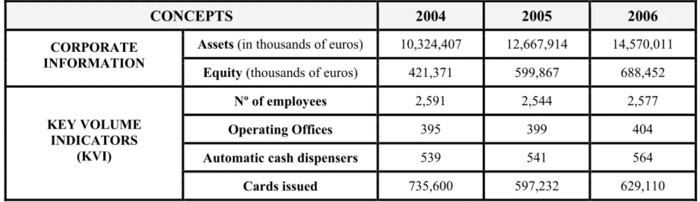
With the object of studying this critical aspect in greater depth, we have focussed our study on testing and analysing the implementation of the Loss Distribution Approach (LDA) by using exclusively the internal loss data provided by a Spanish credit entity, which operates essentially in the retail banking sector. It is necessary first to know the profile of this entity in order to understand better the data and results obtained in the study. Therefore, we have selected a series of descriptive variables covering the three sampling periods (see table 2):
Table 2: Credit entity’s relevant information
CONCEPTS 2004 2005 2006
Assets (in thousands of euros) 10,324,407 12,667,914 14,570,011 CORPORATE
INFORMATION
Equity (thousands of euros) 421,371 599,867 688,452
Nº of employees 2,591 2,544 2,577
Operating Offices 395 399 404
Automatic cash dispensers 539 541 564
KEY VOLUME INDICATORS
(KVI)
Cards issued 735,600 597,232 629,110
The IOLD includes operational events that occurred in each of following seven years, from 2000 to 2006. In table 3, the number of events recorded per year is given:
Table 3: Number of operational risk events per year.
YEAR 2000 2001 2002 2003 2004 2005 2006
Nº EVENTS 2 5 2 50 6,397 4,959 6,580
From the preceding table, it can be inferred that the frequency of events from the year 2000 to 2003 is not significant. Consequently, so as not to distort the distribution of frequency, for the purposes of modelling we shall only consider 2004, 2005 and 2006 as representative years. On this point, the Committee (2006: 168) indicates that the history of operational losses must cover a minimum period of five years. However, the banks that use an AMA methodology for the first time are allowed to use data referring to a period of observation of at least three years, as in the case that concerns us. It should also be noted that inflation, affecting the data for the various periods of years over which it is compiled, can distort the results of the research. To take this effect into account, we have used the CPI
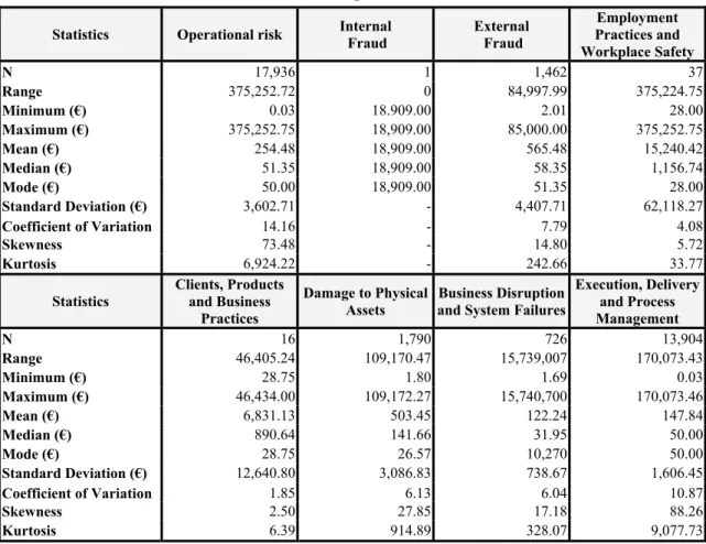
(Consumer Prices Index) to adjust the amount of the losses, taking the year 2006 as the base. Thus we have converted the nominal losses in equivalent monetary units. Further, before implementing any statistical approach, it is essential to perform an EDA (Exploratory Data Analysis) of the data6, in order to analyze the nature of the sample used. In total, it includes 17,936 observations of operational risk events, all classified into seven event types within the retail banking business line. The total sum of the losses for this business unit exceeds 4.5 million Euros, and the distribution of these losses between the different categories of risk is very heterogeneous. The descriptive statistics are given in Table 4 for both the total sample, in the column headed Operational Risk, and for each of the particular event types7. The results obtained are presented in table 4.
Table 4: Descriptive Statistics.
Statistics Operational risk Internal
Fraud External Fraud
Employment Practices and Workplace Safety
N 17,936 1 1,462 37
Range 375,252.72 0 84,997.99 375,224.75
Minimum (€) 0.03 18.909.00 2.01 28.00
Maximum (€) 375,252.75 18,909.00 85,000.00 375,252.75
Mean (€) 254.48 18,909.00 565.48 15,240.42
Median (€) 51.35 18,909.00 58.35 1,156.74
Mode (€) 50.00 18,909.00 51.35 28.00
Standard Deviation (€) 3,602.71 - 4,407.71 62,118.27
Coefficient of Variation 14.16 - 7.79 4.08
Skewness 73.48 - 14.80 5.72
Kurtosis 6,924.22 - 242.66 33.77
Statistics Clients, Products and Business
Practices
Damage to Physical Assets
Business Disruption and System Failures
Execution, Delivery and Process Management
N 16 1,790 726 13,904
Range 46,405.24 109,170.47 15,739,007 170,073.43
Minimum (€) 28.75 1.80 1.69 0.03
Maximum (€) 46,434.00 109,172.27 15,740,700 170,073.46
Mean (€) 6,831.13 503.45 122.24 147.84
Median (€) 890.64 141.66 31.95 50.00
Mode (€) 28.75 26.57 10,270 50.00
Standard Deviation (€) 12,640.80 3,086.83 738.67 1,606.45
Coefficient of Variation 1.85 6.13 6.04 10.87
Skewness 2.50 27.85 17.18 88.26
Kurtosis 6.39 914.89 328.07 9,077.73
6 See Tukey (1977) and Hoaglin et al. (1983 and 1985).
7 In the Internal Fraud category there is only one observation; this prevents any individualised study of this type of risk and, consequently, the application of the LDA model in this cell.
From observing table 4, it should be noted that the mean is, in all the cases, much higher than the median. This fact constitutes a clear sign of the positive asymmetry of the distributions. At the same time, we should warn that the mode takes very relatively small values. Taken together, these two factors denote the grouping of distribution body in a range of low severity values.
In addition, if we assume the standard deviation as a proxy for the dispersion of the data, when a comparison is made of the diverse risks, we could draw incorrect conclusions. This assertion is based on the evident disparity in the mean values of each type of operational risk. To resolve it, we have determined the Pearson coefficient of variation; this is a relative measure of the dispersion that allows us to test it more rigorously. On this basis, we find that the greatest dispersion (10.87) occurs with the cell of Execution, Delivery and Process Management (henceforth Processes); this type of risk accounts for the largest number of events of the sample. In contrast, Employment Practices and Workplace Safety (henceforth Human Resources), which has the largest index of standard deviation (62,118.27 Euros), presents a coefficient of variation of 4.08.
At the same time, the observed values for the shape parameters describe distributions with positive asymmetry and leptokurtosis; however, each type of risk presents a different degree of intensity8 in both measures. More specifically on this aspect, the Processes type of risk has the highest degree of skewness (88.26) and kurtosis (9,077.73), unlike the cell of Clients, Products and Business Practices (henceforth Clients) whose skewness and kurtosis, respectively, are notably lower (2.50 and 6.39). On this point, it should be noted that in the Clients category we have observed some features clearly differentiated from the rest: a low degree of asymmetry and kurtosis, and a very moderate dispersion (1.85). This singular character is due to the very small number of observations recorded, in comparison with other sub-sets of the sample.
In a general sense, but with the reservations indicated, the distributions analyzed confirm an initial assumption: they are characterised by a grouping, in the central body, of low severity values, and a wide tail marked by the occurrence of infrequent but extremely onerous losses. This characteristic can be observed very clearly by considering the percentiles of the different risks, illustrated in table 5.
8 The operational risk as a whole is strongly influenced by the Processes subset. It represents about 77.52% of the total events in the sample.
Table 5: Percentiles of operational risk distribution.
PERCENTILE RISK
5 25 50 75 90 95 99 99.9
External Fraud 20.00 42.60 58.35 155.22 410.46 904.25 7,147.61 85,000.00 Employment Practices
and Workplace
Safety. 72.13 446.18 1,156.74 2,986.04 28,132.74 90,044.77 375,252.75 375,252.75 Clients, Products and
Business Practices 28.75 152.76 890.64 6.067.37 31,184.26 46,434.00 46,434.00 46,434.00 Damage to Physical
Assets 26.57 69.90 141.66 313.35 738.87 1,500.55 7,428.79 66,521.50 Business Disruption
and System Failures 10.00 10.65 31.95 60.00 176.21 308.10 1,386.15 15,740.70 Execution, Delivery
and Process
Management 5.13 18.63 50.00 102.70 213.00 452.00 1,426.01 9,431.14
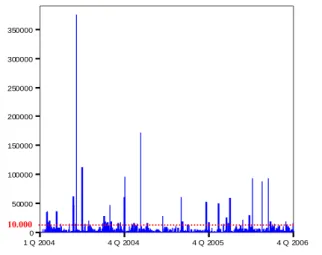
Over the total of the sample, we can conclude that 99% of the operational loss events recorded in the IOLD kept by the bank are of less than 2,548 Euros in value. On this point, the Committee (2006: 168) proposes that banks should compile data on and model only those events that individually exceed a threshold of 10,000 Euros of loss. Currently, given the relatively few events recorded in the IOLD, applying a high threshold could make the advanced measurement model less rigorous, as happens in our study, thus making it impossible to apply the model in some of the cells of the matrix. Our IOLD employs a threshold of 0 Euros for capturing loss events (see figure 1).
Figure 1: Amount of the operational losses recorded in the IOLD.
If a threshold of 10,000 Euros is applied, the frequency of events would be only 22, 7 and 14 for the years 2004, 2005 and 2006, respectively. Consequently, for our modelling, we decided to take a threshold of 0 Euros, equal to that adopted for recording them in the database.
1 Q 2004 4 Q 2004 4 Q 2005 4 Q 2006
0 50000 100000 150000 200000 250000 300000 350000
10.000
4. THE MODEL SELECTION.
4.1FREQUENCY DISTRIBUTION.
The frequency is determined from the number of events that have occurred in a particular period of time, commonly known as the "risk horizon" (Alexander, 2003: 143). For regulatory purposes, this period is set at one calendar year, for operational risk (Basel, 2006: 166). Consequently, if the regulatory capital has to cover the possible losses that the entity may suffer from within one year period, the annual frequency must be modelled in the LDA approach. Given the scarcity of significant periods of samples of operational losses, this requirement presents even more difficulties for implementing this methodology since, as Dutta and Perry (2006: 23) emphasise, with two or three years of losses, it is not possible to perform a consistent analysis of the goodness-of-fit of a theoretical to an empirical frequency distribution.
In such scenario –for our study we have a sample of three years of losses– Fontnouvelle et al. (2004) suggest the Poisson function as the most appropriate distribution. The Poisson formulation is characterised by a single parameter, λ, which represents the mean number of annual events and, at the same time, the variance of the distribution. Thus, if the frequency of the losses is a discrete random variable, N, which follows a Poisson distribution (Po), then:
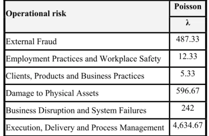
Where, λ>0 (4) Table 6 summarizes the results obtained in the estimation of the parameters for each type of operational risk:
Table 6: Estimated parameters for the frequency distribution Poisson Operational risk
λ
External Fraud 487.33
Employment Practices and Workplace Safety 12.33 Clients, Products and Business Practices 5.33
Damage to Physical Assets 596.67
Business Disruption and System Failures 242 Execution, Delivery and Process Management 4,634.67
4.2SEVERITY DISTRIBUTION.
The Basel Committee (2001) proposed as a benchmark the Lognormal distribution for modelling the severity, and the Poisson distribution for the frequency. Thus, in the initial phases of development of
) ! (
) (
~ x
x e N P Po
N
x λ
λ → = = λ −
the LDA model, a debate took place in the banking industry (which was not reflected in the scientific literature with the same intensity) on whether a Standard LDA Model, "Lognormal and Poisson", should be stipulated in the regulations, with a view to allowing a more homogeneous comparison to be made between the amounts of regulatory capital held by the various banks. With regard to the Lognormal function, we can say that a random variable, X, follows this distribution, if the logarithm of X is normally distributed, that is, if it fits a Normal distribution; its function of density therefore is defined by the following expression:
for x>0, and where μ and σ represent the mean and the standard deviation of the logarithm of the random variable, respectively. However, although the Lognormal distribution is a widely spread probabilistic model, the results derived from empirical studies, such as that conducted by Dionne and Dahen (2007), conclude that the application of the model in leptokurtic scenarios, when this is not the function that obtains the best statistical fit, could lead to the under-valuation of the tail of the aggregate loss distribution and, therefore, of the risk. In consequence, we must undertake a robust study of its suitability, and test it against other possible alternatives to ensure that the Standard LDA Model is the most sensitive, of the models analysed, to the risk assumed. Thus, with the object of evaluating which probabilistic function best fits the severity, we have followed the approach of Dutta and Perry (2006:
22), who establish five key questions: (i) Goodness of Fit; (ii) Realistic outcome; (iii) Well-Specified;
(iv) Flexibility; and (v) Simple.
Regarding the other distributions to be tested, Moscadelli (2004) believes the distribution should be studied in terms of its kurtosis: the Weibull function is proposed for distributions with smooth tail; the Lognormal or the Gumbel function for distributions with moderate or average tail; and, in those with heavy tail, the Pareto function is recommended. On the other hand, Fontnouvelle et al. (2004) widen the possible alternatives, distinguishing two types of distribution: those with smooth tail, for which functions such as the Weibull, Lognormal, Gamma and Exponential are recommended; and the distributions with heavy tail, for which the Pareto, Generalised Pareto, Burr, Log-Logistic and Log- gamma are suggested. In line with the studies cited above, we also have used a range of functions with characteristics that, a priori, are different in respect of the form taken by the tail of their distribution.
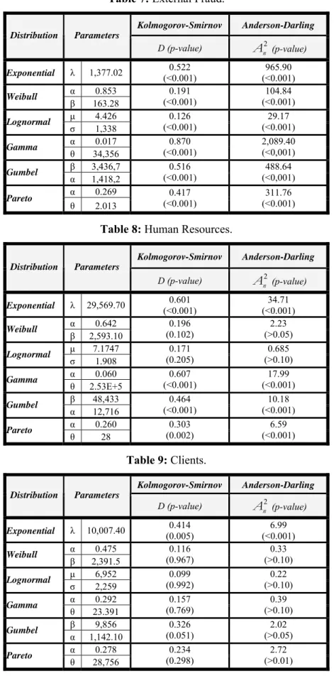
Thus, the suitable functions are the following: Exponential, Gumbel, Gamma, Lognormal, Weibull and Pareto. Having now proposed the candidate functions, the next step is to measure the consistency of the fit. For this purpose, we apply two of the various statistical tests commonly used to determine the probabilistic model followed by the recorded operational losses (see Chernobai et al., 2005). In particular, we conduct the Kolmogorov-Smirnov (K-S) and Anderson-Darling (A-D) tests for calibrating the fit robustness for operational risk event types as illustrate from table 7 to table 12, respectively.
) 5 2 (
) 1 ( ) , (
~ 2
2
2 ) (ln
σ μ
π σ σ
μ
− −
=
→
x
x e x f LN
X
Table 7: External Fraud.
Kolmogorov-Smirnov Anderson-Darling Distribution Parameters
D (p-value) An2 (p-value) Exponential λ 1,377.02 0.522
(<0.001) 965.90 (<0.001) α 0.853
Weibull
β 163.28
0.191 (<0.001)
104.84 (<0.001) μ 4.426
Lognormal
σ 1,338
0.126 (<0.001)
29.17 (<0.001) α 0.017
Gamma
θ 34,356
0.870
(<0.001) 2,089.40 (<0,001) β 3,436,7
Gumbel
α 1,418,2
0.516 (<0.001)
488.64 (<0,001) α 0.269
Pareto
θ 2.013
0.417
(<0.001) 311.76 (<0.001)
Table 8: Human Resources.
Kolmogorov-Smirnov Anderson-Darling Distribution Parameters
D (p-value) An2 (p-value) Exponential λ 29,569.70 0.601
(<0.001) 34.71 (<0.001) α 0.642
Weibull
β 2,593.10
0.196 (0.102)
2.23 (>0.05) μ 7.1747
Lognormal
σ 1.908
0.171
(0.205) 0.685
(>0.10) α 0.060
Gamma
θ 2.53E+5
0.607 (<0.001)
17.99 (<0.001) β 48,433
Gumbel
α 12,716
0.464 (<0.001)
10.18 (<0.001) α 0.260
Pareto
θ 28
0.303 (0.002)
6.59 (<0.001)
Table 9: Clients.
Kolmogorov-Smirnov Anderson-Darling Distribution Parameters
D (p-value) An2 (p-value) Exponential λ 10,007.40 0.414
(0.005) 6.99
(<0.001) α 0.475
Weibull
β 2,391.5
0.116 (0.967)
0.33 (>0.10) μ 6,952
Lognormal
σ 2,259
0.099
(0.992) 0.22
(>0.10) α 0.292
Gamma
θ 23.391
0.157 (0.769)
0.39 (>0.10) β 9,856
Gumbel
α 1,142.10
0.326
(0.051) 2.02
(>0.05) α 0.278
Pareto
θ 28,756
0.234 (0.298)
2.72 (>0.01)
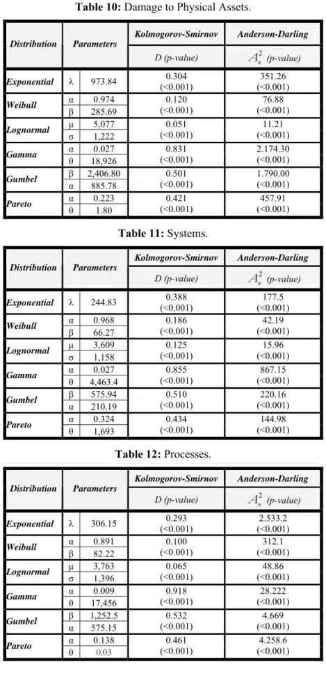
Table 10: Damage to Physical Assets.
Kolmogorov-Smirnov Anderson-Darling Distribution Parameters
D (p-value) An2 (p-value) Exponential λ 973.84 0.304
(<0.001) 351.26 (<0.001) α 0.974
Weibull
β 285.69
0.120 (<0.001)
76.88 (<0.001) μ 5,077
Lognormal
σ 1,222
0.051
(<0.001) 11.21 (<0.001) α 0.027
Gamma
θ 18,926
0.831 (<0.001)
2.174.30 (<0.001) β 2,406.80
Gumbel
α 885.78
0.501 (<0.001)
1.790.00 (<0.001) α 0.223
Pareto
θ 1.80
0.421
(<0.001) 457.91 (<0.001)
Table 11: Systems.
Kolmogorov-Smirnov Anderson-Darling Distribution Parameters
D (p-value) An2 (p-value) Exponential λ 244.83 0.388
(<0.001) 177.5 (<0.001) α 0.968
Weibull
β 66.27
0.186 (<0.001)
42.19 (<0.001) μ 3,609
Lognormal
σ 1,158
0.125
(<0.001) 15.96 (<0.001) α 0.027
Gamma
θ 4,463.4
0.855 (<0.001)
867.15 (<0.001) β 575.94
Gumbel
α 210.19
0.510
(<0.001) 220.16 (<0.001) α 0.324
Pareto
θ 1,693
0.434 (<0.001)
144.98 (<0.001)
Table 12: Processes.
Kolmogorov-Smirnov Anderson-Darling Distribution Parameters
D (p-value) An2 (p-value) Exponential λ 306.15 0.293
(<0.001)
2.533.2 (<0.001) α 0.891
Weibull
β 82.22
0.100
(<0.001) 312.1 (<0.001) μ 3,763
Lognormal
σ 1,396
0.065 (<0.001)
48.86 (<0.001) α 0.009
Gamma
θ 17,456
0.918
(<0.001) 28.222 (<0.001) β 1,252.5
Gumbel
α 575.15
0.532 (<0.001)
4.669 (<0.001) α 0.138
Pareto
θ 0.03
0.461
(<0.001) 4.258.6 (<0.001)
From the results presented in the tables above, and in a broad sense, the limited degree of significance reached in the tests is emphasised. Both the inherent nature of the operational losses and the lack of depth of the data samples, make difficult to find statistical fits with a reasonable degree of significance in practice. According to the regulatory framework, the supervisor must validate the minimum degree of significance established by the entity for selecting the distribution of severity. In our study, in those cases where the fit is poor, we have based our decision on the value of the statistic itself. However, to support the choice of the distribution and, therefore, to avoid the model risk, we considered to seek further support from graphic tools such as P-P Plots. The only types of operational risk that obtain fits better than 1% of significance are Human Resources and Clients. For the rest of the cells, the bias observed between the test statistics and the respective critical values is wide, resulting in some very low p-values. It should be stated that the largest differences arise in the A-D test, due to the greater weight that this test assigns to the deviation in the tail between the estimated and the empirical distribution. This finding coincides with the warning given in the study by Moscadelli (2004).
When establishing a hierarchy of the distributions based on the statistical adjustment, the Lognormal and the Weibull, in that order, are the distributions that present greater significance in all the cases.
Regarding the Pareto distribution, which is suitable for modelling heavy tails, it fits properly for shape parameter values lower than one. This results in infinite moments that could give rise to unrealistic financial measurements in terms of capital. However, this distribution obtains the third best fit in the cells of External Fraud, Human Resources and Systems, although, in this last cell, the Exponential function obtains a better result with the K-S test. It should be mentioned that this function is a particular case of the Weibull when the shape parameter, α, of this latter distribution is equal to one.
Lastly, we have confirmed that the Gamma function, which only obtains a good fit for the Clients event type, and the Gumbel function are those that are furthest, on average, from the pattern of the various empirical distributions. To reinforce the conclusions obtained from both K-S and A-D statistical tests, we have drawn, for each cell, a P-P Plot that shows, comparatively, the three theoretical distributions with better fit (see figure 2).
P-P Plot
Lognormal Pareto Weibull Observed cumulative probability
1 0,8 0,6
0,4 0,2
Expected cumulative probability 0 1 0,9 0,8 0,7 0,6 0,5 0,4 0,3 0,2 0,1 0
P-P Plot
Lognormal Pareto Weibull
Observed cumulative probability0,4 0,6 0,8 1 Expected cumulative probability 0,2
1 0,9 0,8 0,7 0,6 0,5 0,4 0,3 0,2 0,1 0
P-P Plot
Lognormal Pareto Weibull
Observed cumulative probability0,4 0,6 0,8 1 Expected cumulative probability 0,2
1 0,9 0,8 0,7 0,6 0,5 0,4 0,3 0,2 0,1 0
P-P Plot
Exponential Lognormal Weibull
Observed cumulative probability0,2 0,4 0,6 0,8 1 Expected cumulative probability 0
1 0,9 0,8 0,7 0,6 0,5 0,4 0,3 0,2 0,1 0
P-P Plot
Lognormal Pareto Weibull
Observed cumulative probability0,4 0,6 0,8 1 0,2
Expected cumulative probability 10 0,9 0,8 0,7 0,6 0,5 0,4 0,3 0,2 0,1 0
P-P Plot
Exponential Lognormal Weibull
Observed cumulative probability0,2 0,4 0,6 0,8 1 Expected cumulative probability 0
1 0,9 0,8 0,7 0,6 0,5 0,4 0,3 0,2 0,1 0
Figure 2: P-P Plot for the event type.
External Fraud Human Resources
Clients Damage to Physical Assets
Systems Processes
The figure 2 points out the results of the tests, showing that the Lognormal distribution is the theoretical function closest to the plot of the empirical distribution, for all the cells analysed.
Consequently, this distribution has been selected for modelling the severity of operational losses in the LDA structure.
5. REGULATORY CAPITAL FOR OPERATIONAL RISK.
5.1THE STANDARD LDAMODEL.
Having characterised the distributions of frequency and severity, the next step is to determine the aggregate loss distribution and we have chosen the Monte-Carlo Simulation technique to perform the convolution of both frequency and severity distribution. In particular, for each of the convolutions performed, one million simulations have been generated, and relative errors considerably below 1%
have been obtained. When the LDA distribution has been determined, the OpVaR (that is, the 99.9 percentile) must be calculated to infer the regulatory capital. This study has been carried out under the assumption that the credit entity has not made provision for its expected loss (EL). Consequently, the capital requirements have to cover both this loss and the unexpected loss (UL); thus we can identify the figure of the OpVaR with the amount of the Capital at Risk (CaR). The results obtained, after aggregating the two distributions, are shown in table 13:
Table 13: CaR Estimation by the Standard LDA Model.
Lognormal Poisson Event Type
µ σ λ
Expected Loss (euros)
Unexpected
Loss (euros) CaR99.9
(euros)
External Fraud 4.426 1.338 487.33 99,712 48,850 148,562
Employment Practices and
Workplace Safety. 7.174 1.908 12.33 99,405 1,773,522 1,872,927
Clients, Products and Business
Practices 6.952 2.259 5.33 71,459 3,223,149 3,294,608
Damage to Physical Assets 5.077 1.222 596.67 201,766 66,553 268,319 Business Disruption and System
Failures 3.609 1.158 242 17,473 8,748 26,221
Execution, Delivery and Process
Management 3.763 1.396 4,634.67 528,987 75,128 604,115
Global Computation for the Entity 1,018,804 5,195,951 6,214,756
With reference to the CaR figures detailed in table 13, the amount included in the Human Resources cell and, essentially, that in the Clients cell, should be noted 9. In this latter cell, the regulatory capital determined is more than three million Euros; in the Human Resources cell, the capital requirement is close to two million Euros. Paradoxically, although these two cells have the fewest observations, they account for the largest amounts of capital.
9 In the Clients cell, there are only 16 observations recorded. Such a low number of events can distort the financial reality of the results derived; hence certain doubts would be raised regarding its regulatory validation.
The explanation for such differences in terms of capital charge must be sought in the characterisation of the respective probabilistic functions of severity. Thus, in both the Human Resources and Clients cells, where there are risks of low frequency and high severity, the theoretical levels of asymmetry and kurtosis are very high; these values are conditioned by the shape parameter (σ) of the Lognormal distribution. Equally, if we observe their scale parameter (µ), these are high (7,174 and 6,952, respectively) for the event types mentioned and, therefore, the mean and the variance of the severity of their losses are also high in relation to the other types of risk that obtained lower parameters in the probabilistic fit. On the other hand, in the Processes cell, with a mean annual frequency of more than four thousand events, but with shape and scale parameters of their severity function much lower than those indicated in the two previous distributions, the amount of Capital at Risk obtained is only about 600,000 Euros. All this justifies a greater weighting of the distribution of severity, with respect to that of frequency, in the final estimation of the CaR (see Böcker and Klüppelberg, 2005; and De Koker, 2006).
5.1.1 The Expected Loss and the Unexpected Loss
The total amount of regulatory capital assigned to a cell can be broken down into two amounts: the expected loss (EL) and the unexpected loss (UL). Based on this, we introduce two ratios "EL/OpVaR"
and "UL/OpVaR", both representing a measurement of the relative weight of each variable in the total Capital in Risk. Table 14 gives the two ratios calculated for each type of risk.
Table 14: EL/CaR and UL/CaR ratios
The ratios calculated denote two very different situations: (i) for those risks with low or medium severity and high or medium frequency, EL is much higher than UL; (ii) in contrast, those risks with high severity and low frequency, that is, with a greater dispersion of their operational losses, the UL
RATIOS EVENT TYPES
EL/CaR99.9 UL/CaR99.9
External Fraud 67.12% 32.88%
Employment Practices and Workplace
Safety. 5.31% 94.69%
Clients, Products and Business Practices 2.17% 97.83%
Damage to Physical Assets 75.20% 24.80%
Business Disruption and System Failures 66.64% 33.36%
Execution, Delivery and Process
Management 87.56% 12.44%
Global Computation for the Entity 16.39% 83.61%
accounts for almost the total CaR. Given the weight of the Human Resources and Clients, EL only accounts for 16.39% of the total CaR. In consequence, if the entity were able to identify, a priori, the expected loss and make it adequate provisioned, its regulatory capital should rise to 83.61% of the total CaR.
5.1.2 Financial Impact of the Percentile proposed by the Committee.
In regulatory terms, the percentile of the distribution of aggregate losses that determines the Capital at Risk is well-established at 99.9%. The fact that the Committee has recommended such a high figure has aroused criticism and a certain apprehension in the banking sector. Given the leptokurtic character of operational losses, this percentile may lead to an overestimation of the capital required, and may even represent an unsustainable amount in the capital structure of a credit entity. However, the intention of the Committee is precisely to cover the risk of possible extreme losses situated in the tail of the distribution. In order to calibrate the impact of the percentile, we have compared the CaR calculated at the 99.9 percentile (reflected in table 13) with that obtained by applying other less conservative confidence intervals, that is, 90%, 95% and 99%, which are commonly used in the determination of the Value at Risk (VaR) in market risk. Table 15 gives the quantities 10 resulting from the application of each of the percentiles selected.
Table 15: CaR Estimation for different confidence intervals Percentile
Event Type
90 95 99
External Fraud 113,900
(-23.33%) 118,892
(-19.97%) 129,936
(-12.54%)
Employment Practices and
Workplace Safety. 207,127
(-88.94%) 292,606
(-84.38%) 639,607
(-65.85%)
Clients, Products and Business
Practices 156,611
(-95.25%) 255,852
(-92.23%) 793,335
(-75.92%)
Damage to Physical Assets 224,311
(-16.40%) 231,727
(-13.64%) 247,005
(-7.94%)
Business Disruption and System
Failures 20,315
(-22.52%)
21,277
(-18.86%)
23,295
(-11.16%)
Execution, Delivery and Process
Management 555,061
(-8.12%)
563,887
(-6.66%)
580,744
(-3.87%)
Global Computation for the
Entity 1,120,716
(-81.97%) 1,228,392
(-80.23%) 2,515,510
(-59.52%)
The estimation of the CaR, illustrated in table 15, demonstrates the conservative effect of the regulatory percentile on the Capital at Risk. However, it can be seen from the results that this impact on the capital requirement becomes greater when the degree of kurtosis and the dispersion of the fitted severity distributions are both greater. It should be noted that, in the Processes cell, which presents the
10 The percentage figures situated below the absolute value express the reduction with respect to CaR99.9% .
highest frequency recorded, the capital saving when comparing the 90 percentile with respect to the 99.9 percentile only reaches 8.12%, in relative terms.
On the other hand, it is observed that the External Fraud risk presents reductions in the CaR of 23.33%, 19.97% and 12.54% for the 90%, 95% and 99% confidence intervals, respectively. In the Systems cell the previous estimations are practically replicated, while in the Damage to Physical Assets cell they are slightly lower. In contrast, in the Human Resources and Clients event types, the differences are much more extreme. For example, by setting a confidence interval of 99%, the capital saving would reach 65.85% for Human Resources, and 75.92% for Clients risks; if the confidence interval was 90%, the differences indicated would be 88.94% in the first event type, and 95.25% in the second one.
Again, when the data are summed for the entity as a whole, the weighting of the risks of low frequency and high severity ceases to be noted, since the total amount is found to vary, in decreasing order, by 81.97%, 80.23% and 59.52%, for the 90, 95 and 99 percentiles, respectively. More specifically, when the percentile is 99 –only 0.9 less than the regulatory level– the capital at risk would fall from 6,214,756 Euros to 2,515,510 Euros.
5.2NON-ADVANCED METHODOLOGIES.
With the aim of comparing the capital savings resulting from the application of the LDA approach with that obtained using non-advanced methodologies, we have calculated the regulatory capital in accordance with the Basic (BIA) and Standardised (SA) models. In part 2, we detail the technical aspects of these two capital measurement methodologies. Both the BIA and the SA approaches cover operational risk with a capital amount equivalent to a fixed percentage of the so called exposure indicator. The principal difference between these two methods is that, in the Standardised Approach, the total amount of capital required is calculated as the sum of the regulatory capital requirements of each of the eight business lines described by the Basel Committee.
The Exposure Indicator
The Committee (2004: 129) has proposed the Gross Income variable as a proxy for the size or level of exposure to operational risk. Since the banking business of the credit entity analysed consists almost entirely of Retail Banking, to determine the Gross Income we have used the information contained in the Profit & Loss Account without consolidating it to group level.
Table 16 shows the make-up of the Gross Income figure:
Table 16: Gross Income.
CONCEPTS 2004 2005 2006
Assimilated Interest and Income 449,473 485,297 566,314
Assimilated Interest and Expenses -193,002 -216,581 -286,108
Income from Capital Instruments 8,476 79,116 71,756
Commissions Received 77,254 87,374 95,515
Commissions Paid -4,129 -7,481 -8,078
Results of Financial Operations 24,716 24,675 19,573
Other income from operations 6,739 7,457 9,581
Gross Income 369,527 459,857 468,553
*Figures in thousands of Euros
Average Gross Income:
n GI GI
n
i
n average
∑
== 1
1...
= 432,646,000 Euros.
The Regulatory Capital (K)
In the Basic Method a multiplier of 15% is set for the aggregate business of the bank. However, in the Standardised method, a different factor is taken for each business line; in the case of Retail banking the coefficient is set at 12% (see table 1). The calculations made are detailed below:
Basic Indicator Approach: KBIA=(average gross income x 15%) = 64,897,000 Euros.
Standard Approach: KSA= (average gross income x 12%). = 51,917,000 Euros.
Comparing the capital amounts obtained from the BIA and SA approaches with that resulting from the LDA model, a notable divergence can be appreciated. In particular, the underlying saving of capital from applying the LDA model compared with the Basic and Standardised Methods is 90% and 88%, respectively, as noticed from figure 3.The Committee (2006: 14) recommends banking supervisors to set “prudential floors” in those entities that adopt the AMA methodologies. In particular, it wants minimum coefficients of capital to be established, with the purpose of ensuring the correct application of the advanced methods in each bank. These minima may be based on a proportion of the capital
0 10.000 20.000 30.000 40.000 50.000 60.000 70.000
Capital Regulatorio (Miles de Euros)
BIA SA LDA
estimated by a non-advanced approach. Thus, in principle, the Committee (2001: 18) determined that the measurement of capital obtained by using an AMA approach could not be less than 75% of the amount of capital required obtained by the Standardised Approach; the CaR resulting from our Standardised LDA Model is far less than this minimum threshold. However, the delimitation of this minimum quota will be the competence, ultimately, of the national supervisor.
Figure 3: Capital charge comparison.
6. CONCLUSIONS.
The main aim of this paper is to highlight the existing divergences in the estimation of regulatory capital for operational risk associated with different methodologies proposed by the Committee, taking a Spanish financial entity as an example. In particular, we illustrate the potential benefit derived from implementing an advanced measurement approach, the LDA, versus the Basic and Standardised methods.
Thus, we have warned that the non-advanced approaches show some extremely conservative results;
their capital charges are proportional to the entity’s business volume, so that, in cycles of flourishing economic activity, the regulatory capital is expected to increase, independently of the scale of the risk controls established by the entity. However, it must also be noticed that the LDA model presented, based on a loss database of only three years (and possibly incomplete, too, especially for cases of Internal Fraud), may not reach the minimum coefficient of capital that the supervisor suggests for the implementation of AMA methodologies.
From a methodological perspective, the Basic and Standardised approaches present certain conceptual deficiencies, particularly with reference to their proposed exposure indicator, the entity's Gross Income; this is because this variable depends on the accounting systems of each country, and