© 2013 Ospina-Noreña et al., licensee InTech. This is an open access chapter distributed under the terms of the Creative Commons Attribution License (http://creativecommons.org/licenses/by/3.0), which permits unrestricted use, distribution, and reproduction in any medium, provided the original work is properly cited.
Effects of Climate Change on Hydric Resources:
Some Implications and Solutions
Jesús Efren Ospina-Noreña, Carlos Gay García, Ana Elisa Peña del Valle and Matt Hare
Additional information is available at the end of the chapter http://dx.doi.org/10.5772/54774
1. Introduction
Among the issues that humanity currently faces and will face in the future, the scarcity of water and the onset of large-scale events linked to it – such as the increasingly frequent periods of protracted drought and heavy flooding in different regions of the world – are undoubtedly some of the most pressing. Accordingly, these conditions will have to be considered in the modeling and analysis of water supply and demand in the coming years.
As the distribution and growth of the world population runs parallel both to the increasing demand for water for different uses and the potential reduction of natural resources, these are important factors that hereafter will affect the availability of the liquid for human consumption.
Section 1, in describing the impact of climate change on the availability and distribution of water resources, analyzes this phenomenon under different models and scenarios of greenhouse gases emissions; section 2 refers to and documents the implications of water availability in different regions, taking into account the various production and development sectors; lastly, in section 3 we discuss some cases of adjustment policies implemented through the adaptive management approach (implemented in recent years in different parts of the world).
The first section of the present chapter yields some relevant results from the research that has been advanced at the Centro de Ciencias de la Atmósfera (CCA) [Center for Atmospheric Sciences] and the Programa de Investigación en Cambio Climático (PINCC) [Climate Change Research Program] of the Universidad Nacional Autónoma de México (UNAM) [National Autonomous University of Mexico], based on the modeling of climate change in different regions and covering various aspects, notably the situation of productive and development sectors vis-à-vis water resources.
The chapter provides, among other items, the findings derived from modeling the potential impact of climate change on the availability of water and the degree of pressure exerted on water resources in four hydrological-administrative regions of the Comisión Nacional del Agua (CNA) [National Commission of Water] in the Gulf of Mexico Basin, with the corresponding documentation. In depicting the vulnerability of water resources in the Guayalejo-Tamesí River Basin due to climate change, it highlights the effects of this phenomenon on irrigation districts (e.g., the downturn it has brought about in the supply/demand rate). The scenarios contemplate the coverage of demand, the supply requirements, and the unmet requests in the region. Likewise, the consequences of capturing rainwater for irrigation purposes in a pilot project based in San Miguel de Allende, Mexico, are discussed in the context of strategies for adapting to climate change.
The chapter in question also seeks to address important issues regarding the potential impact of climate change on the hydropower sector by focusing on the relationship of water supply/demand in the Sinú-Caribe River Basin in Colombia. In doing so, it analyzes briefly the eventuality that water resources embody a limiting factor in the course of time for different activities in the region, and provides at the end a series of observations that can help to plan and establish guidelines for the different production and development sectors.
Finally, the chapter points to the importance of adaptive schemes for the sustainable management of water resources under scenarios of high uncertainty and complexity.
Moreover, by using several examples from the international realm on the adaptive management of water, this section shall show how the participatory-laden management of public policies, in conjunction with the measures referred to as "flexible," can effectively address several of the dilemmas as regards to water resources and the natural hazards that accompany climate change.
2. Models and scenarios of climate change
In order to observe the effects of climate change on hydric resources, it is necessary to work out future scenarios of those variables that become more relevant or influential as far as the availability of water is concerned, such as: temperature (T), precipitation (PCP), and evaporation (Ev), among others
Nowadays, there are several joint models (Atmosphere/Ocean General Circulation Model [AOGCM]) that are run under different scenarios of greenhouse gases emissions, which result in a wide range of future scenarios on a global and regional scale with respect to climate variables. This allows us to pose different projections whereby multiple analyses are facilitated and solid tools are generated for decision makers. At the same time, however, there appears a high degree of uncertainty and complexity – something that one must take into account when studying the impact of climate change on water availability, as the present chapter intends to do.
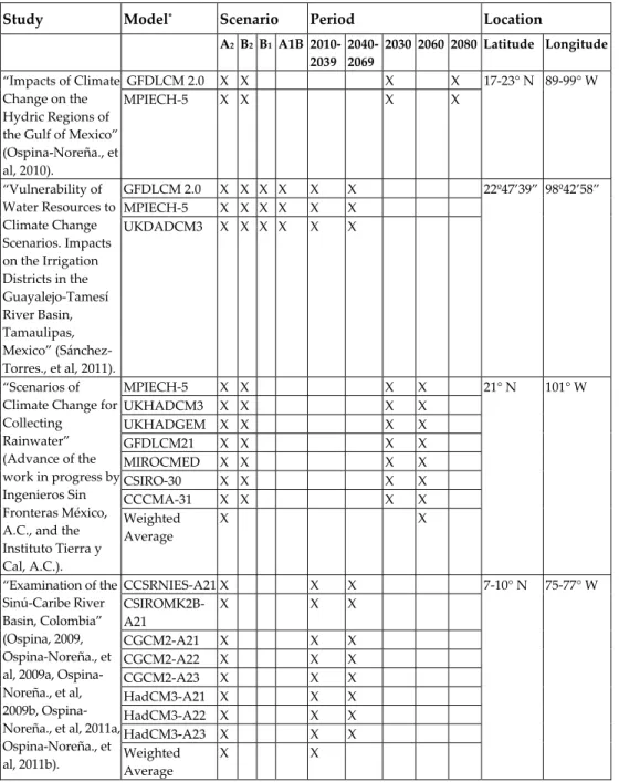
The afore mentioned studies are relying on some models and have considered different periods of analysis; this information is given in Table 1, which includes the approximate location of the projects. Table 2 briefly describes the patterns of the various scenarios that have been used.
3. Methodological aspects
In each one of these studies, the projections of climate change’s effects on the availability of hydric resources were estimated mainly by adjusting the averages for the mean temperature (meaT), the highest temperature (maxT), and precipitation (PCP) (base lines) taking into account the most representative weather stations that can be found within and/or close to the corresponding areas under scrutiny, while the projections about the anomalies to be ascribed to each region were provided by the program known as MAGICC/SCENGEN1 v.5.3, and the outlets of the experiments carried out by the Canadian Institute for Climate Studies (CICS) for the models presented in Table 1.
For the analysis of hydric resources, each one of the projects had to use a different and, indeed, numerous series of variables and relations, namely the current availability (or natural offer) of water; evaporation; flow or expenses; the P/T (Precipitation/ Temperature) relationship or Lang Index (IL); the supply/demand relation; the projections made for hydric resources, for its demand, and for the population; the index of pressure on the resource, etc.
More details about the information on models, scenarios, tools, back-up software, and the methodologies used can be found in: (Sánchez-Torres., et al, 2011; Ospina-Noreña., et al, 2009a; Ospina-Noreña., et al, 2009b; Ospina-Noreña., et al, 2010; Ospina-Noreña., et al, 2011a;
Ospina-Noreña., et al, 2011b).
Furthermore, for the information concerning greenhouse gases (GHG) emissions, global climate models or general circulation models (GCMs), programs known as climate scenario generators, and relevant conceptualizations of climate change, we refer to Wigley (1994), Wigley (2003), Hulme, et al (2000), Conde (2003); as for the examination of vulnerability and the effects on different sectors, see Gay (2000).
4. Results
4.1. Trends and future scenarios
As for the regions on which the studies referred to in this chapter are concentrated, the climate change scenarios show a tendency to the rise of the mean temperature and the highest temperature in each case. Regarding precipitation, the projections indicate slight to substantial increases or decreases in a given region (Tables 3, 4, 5, 6), which implies a high degree of uncertainty in the results – something that will have to be assessed.
1 Authors such as Wigley (1994), Wigley (2003), Hulme., et al (2000),Conde (2003) point out that there are simple climate models which incorporate the gamut of emissions scenarios to the studies of climate change. According to them, these models can simulate the response of global climate to changes in the concentrations of greenhouse gases (GHG) in terms of an increment in temperature and the rise of the sea level. One of them is the model for the evaluation of greenhouse gases effects that is designated as the Model for the Assessment of Greenhouse-Gas Induced Climate (MAGICC). However, for the results of MAGICC to be combined with the outlets of general circulation models (GCMs), it is necessary to use the climate scenario generator called SCENGEN (Regional Climate SCENarioGENerator).
Study Model* Scenario Period Location A2B2B1A1B 2010-
2039 2040- 2069
2030 2060 2080 Latitude Longitude
“Impacts of Climate Change on the Hydric Regions of the Gulf of Mexico”
(Ospina-Noreña., et al, 2010).
GFDLCM 2.0 X X X X 17-23° N 89-99° W
MPIECH-5 X X X X
“Vulnerability of Water Resources to Climate Change Scenarios. Impacts on the Irrigation Districts in the Guayalejo-Tamesí River Basin, Tamaulipas, Mexico” (Sánchez- Torres., et al, 2011).
GFDLCM 2.0 X X X X X X 22º47’39” 98º42’58”
MPIECH-5 X X X X X X
UKDADCM3 X X X X X X
“Scenarios of Climate Change for Collecting Rainwater”
(Advance of the work in progress by Ingenieros Sin Fronteras México, A.C., and the Instituto Tierra y Cal, A.C.).
MPIECH-5 X X X X 21° N 101° W
UKHADCM3 X X X X
UKHADGEM X X X X
GFDLCM21 X X X X
MIROCMED X X X X
CSIRO-30 X X X X
CCCMA-31 X X X X
Weighted Average
X X
“Examination of the Sinú-Caribe River Basin, Colombia”
(Ospina, 2009, Ospina-Noreña., et al, 2009a, Ospina- Noreña., et al, 2009b, Ospina- Noreña., et al, 2011a, Ospina-Noreña., et al, 2011b).
CCSRNIES-A21 X X X 7-10° N 75-77° W CSIROMK2B-
A21
X X X
CGCM2-A21 X X X
CGCM2-A22 X X X
CGCM2-A23 X X X
HadCM3-A21 X X X
HadCM3-A22 X X X
HadCM3-A23 X X X
Weighted Average
X X
*Generally, the designation of the models is based on the root or the initials of the institute in charge of the climate modeling; e.g., Geophysical Fluid Dynamics Laboratory (GFDL), Canadian Climatic Center Model (CCCM), National Center for Atmospheric Research (NCAR).
Table 1. Models and Scenarios Used in the Studies.
Scenario Families
Description
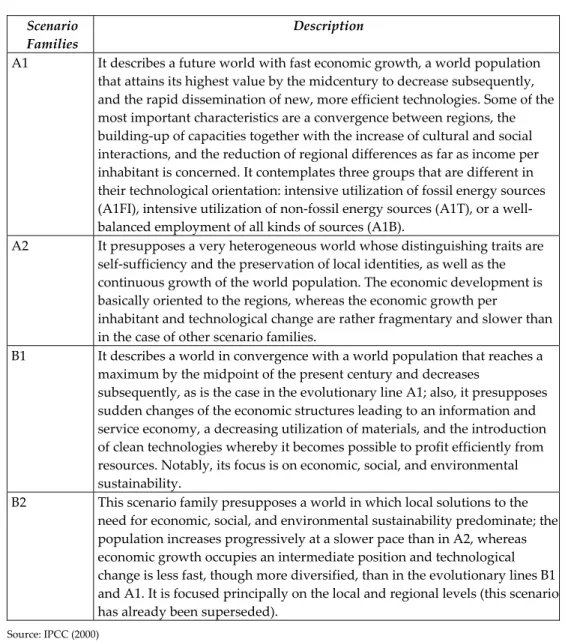
A1 It describes a future world with fast economic growth, a world population that attains its highest value by the midcentury to decrease subsequently, and the rapid dissemination of new, more efficient technologies. Some of the most important characteristics are a convergence between regions, the building-up of capacities together with the increase of cultural and social interactions, and the reduction of regional differences as far as income per inhabitant is concerned. It contemplates three groups that are different in their technological orientation: intensive utilization of fossil energy sources (A1FI), intensive utilization of non-fossil energy sources (A1T), or a well- balanced employment of all kinds of sources (A1B).
A2 It presupposes a very heterogeneous world whose distinguishing traits are self-sufficiency and the preservation of local identities, as well as the continuous growth of the world population. The economic development is basically oriented to the regions, whereas the economic growth per
inhabitant and technological change are rather fragmentary and slower than in the case of other scenario families.
B1 It describes a world in convergence with a world population that reaches a maximum by the midpoint of the present century and decreases
subsequently, as is the case in the evolutionary line A1; also, it presupposes sudden changes of the economic structures leading to an information and service economy, a decreasing utilization of materials, and the introduction of clean technologies whereby it becomes possible to profit efficiently from resources. Notably, its focus is on economic, social, and environmental sustainability.
B2 This scenario family presupposes a world in which local solutions to the need for economic, social, and environmental sustainability predominate; the population increases progressively at a slower pace than in A2, whereas economic growth occupies an intermediate position and technological change is less fast, though more diversified, than in the evolutionary lines B1 and A1. It is focused principally on the local and regional levels (this scenario has already been superseded).
Source: IPCC (2000)
Table 2. Characteristics of the Scenario Families.
Although the estimates used in the projections of climate change’s effects on water resources availability for each one of the CNA’s hydrological-administrative regions (see, Attached Document I) and in the study on the collection of water were applied every five years, herein we will present only some relevant results regarding the periods mentioned in Table 1. Table 3 registers a slight increase in region XII (the Yucatán Peninsula) that was provided by model GFDLCM2.0 for scenarios A2 and B2, as well as small decreases for the rest of the regions, region IX (Northern Gulf) being the most affected, as it reaches a decrease of 10.8%
in scenario A2 and 4.3% in scenario B2 for 2080. On the other hand, model MPIECH-5 for the A2 and B2 scenarios projects important reductions of precipitation in regions XII (-21.1%
and -14.7% for scenarios A2 and B2, respectively, by 2080) and XI Frontera Sur (-26.4% and - 18.5 for scenarios A2 and B2, respectively, by 2080), together with slightly minor diminutions in regions X (Central Gulf) and IX.
We can deduce from Table 4 that in the Guayalejo-Tamesí River Basin precipitation displays a tendency downwards, whereas temperature shows a tendency upwards, which in turn provokes a decrease in the P/T relationship or Lang Index (IL) , used to determine the kind of year (very humid, humid, normal, dry or very dry); thus allowing the remark that for the period of 2010-2069 virtually no humid or very humid years are expected at the Guayalejo- Tamesí River Basin, the temperature sticking to normal and with trends towards dry and very dry days as time goes by. Again, though in this study the projections were undertaken year after year and for four emission scenarios (Sánchez-Torres., et al, 2011), the only findings that are presented correspond to scenarios A2 and B2 during the span of a decade and for the end of the periods reported in Table 1.
Year/Mod Region XII1 Region XI2
GFDLCM20-A2 GFDLCM20-B2 GFDLCM20-A2 GFDLCM20-B2
% changePrec
Change meaT
(°C)
% changePrec
Change meaT
(°C)
% changePrec
Change meaT
(°C)
% changePrec
Change meaT
(°C)
2030 4.7 0.5 4.3 0.6 0.26 0.51 0.5 0.58
2080 11.4 2.0 7.8 1.5 -2.77 2.02 -2.2 1.53
MPIECH-5 A2 MPIECH-5 B2 MPIECH-5 A2 MPIECH-5 B2
2030 -6.6 0.7 -4.75 0.8 -7.87 0.85 -6.07 0.86
2080 -21.1 2.7 -14.67 2.0 -26.35 3.02 -18.48 2.22
Region X3 Region IX4
GFDLCM20-A2 GFDLCM20-B2 GFDLCM20-A2 GFDLCM20-B2
2030 -1.66 0.49 0.02 0.56 -8.1 0.53 -2.2 0.66
2080 -2.9 1.9 -1.24 1.44 -10.81 2.08 -4.3 1.59 MPIECH-5 A2 MPIECH-5 B2 MPIECH-5 A2 MPIECH-5 B2 2030 -2.82 0.84 -0.92 0.84 -6.68 0.79 -1.00 0.9
2080 -6.26 2.9 -3.56 2.12 -6.7 2.85 -1.47 2.1
1 Current mean precipitation: 1,226.7, current mean temperature: 26.5°C, current P/T: 46.3
2 Current mean precipitation: 2,105.2, current mean temperature: 26.9°C, current P/T: 79.1
3 Current mean precipitation: 1,755.9, current mean temperature: 23.6°C, current P/T: 79.4
4 Current mean precipitation: 1,349.3, current mean temperature: 24.1°C, current P/T: 56.8
Table 3. Anomalies of Precipitation and Mean Temperature for the Four Hydrological-Administrative Regions.
Year GFDLCM2.0-A2 GFDLCM2.0-B2
meaT£ PCP€ P/T % change* meaT PCP P/T % change*
2039 25.6 764.1 29.9 -9.6 25.7 810.1 31.6 -4.6 2069 26.4 754.5 28.6 -13.4 26.2 802.8 30.7 -7.1
MPIECH-5-A2 MPIECH-5-B2
2039 26.0 751.9 28.9 -12.6 26.0 800.6 30.8 -7.0 2069 27.2 731.9 26.9 -18.6 26.8 786.7 29.4 -11.0
£ Base line: 25°C, € Base line: 826.5 mm, *With respect to the current value of P/T equal to 33.06.
Table 4. Climate Projections for the Study on the Irrigation Districts in the Guayalejo-Tamesí River Basin, Tamaulipas, México.
As is shown by the results of the study “Scenarios of Climate Change for Rainwater Collection” (prepared by Ingenieros Sin Fronteras México, A.C., and the Instituto Tierra y Cal, A.C, 2012), in the case of the A2 scenarios only one model, the GFDLCM21_A2, projects an increase in precipitation, that is, here 85.7% of the models analyzed indicate that a decrease in precipitation is highly likely; nevertheless, all the models are equally likely to occur. Therefore, our proposal is to generate the weighted average scenario, which takes into account the results of all the models and is meant to operate as a planning platform for the collection of rainwater or the availability of this resource, so as to avoid the most adverse effects. The two models that thoroughly undermine the objectives and aims of the project would be the CCCMA-31 and the CSIRO-30 (see Table 5).
As for the B2 scenarios, there are three (42.9%) where an increase is projected and four (57.1%) where a decrease in precipitation is foreseen; however, two of the three models that project an increase are almost insignificant, as can be observed in Table 5 – something that once again highlights the tendency toward a decrease in precipitation in the project’s study or influential area.
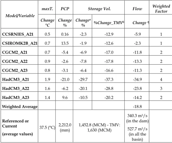
Regarding the research into the Sinú-Caribe River Basin in Colombia, the findings show a tendency to the rise in the highest temperature, and slight to substantial increases or decreases of the PCP, which leads to the reduction of water availability, the effects projected by model HadCM3 being the most adverse (see Table 6).
4.2. The effect of climate change on water availability and pressure degree in the Gulf of Mexico
Relying on the projections for precipitation and the mean temperature, the Lang Index was calculated for the four scenarios that were obtained from running the models GFDLCM2.0 and MPIECH-5 for each one of the Gulf of Mexico’s hydrological-administrative regions.
Such index can be interpreted as one measuring the degree of aridity or humidity that predominates in the various regions. Starting from the P/T relationship’s current values that are shown in Table 3, we determined the percentage of rise or diminution of such relation (see Table 7) according to the different projections – an amount that in turn is assumed to represent an increase or decrease in the availability of hydric resources.
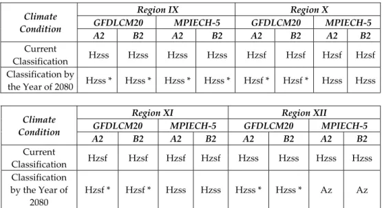
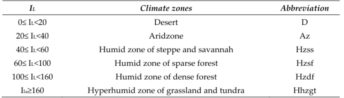
The findings presented in Table 7 (which follow the classification set in Table 8) allow us to establish a change in trend in the climate zones of each hydrological-administrative region, as is shown also in Table 9. For example, in region XII a humid zone of steppe and savannah (Hzss) would turn into an arid zone (Az), whereas in regions XI and X humid zones of sparse forest (Hzsf) would become humid zones of steppe and savannah (Hzss). These figures were obtained as projected by the model MPIECH-5 for scenarios A2 and B2.
Year
UKHADGE M_A2
UKHADC M3_A2
MPIECH- 5_A2
GFDLCM21 _A2
MIROCME D_A2
CSIRO- 30_A2
CCCMA- 31_A2
WA_
A2£
Change (%)
Change (mm)
Change (%)
Change (mm)
Change (%)
Change (mm)
Change (%)
Change (mm)
Change (%)
Change (mm)
Change (%)
Change (mm)
Change (%)
Change (mm)
Change (mm)
2030 -5.2 479.4 -1.9 496.1 -3.4 488.3 8.4 548.0 -2.6 492.7 -5.9 476.0 -8.7 461.7 482.1 2060 -10.0 455.1 -3.0 490.3 -6.3 473.7 18.5 599.3 -4.5 482.9 -11.4 447.9 -17.3 417.9 460.7 Weighted
Factor 3 2 3 1 2 4 5
Change through 2060€
-50.5 -15.3 -31.9 93.7 -22.7 -57.7 -87.7 -44.9
UKHADGE M_B2
UKHADC M3_B2
MPIECH- 5_B2
GFDLCM21 _B2
MIROCME D_B2
CSIRO- 30_B2
CCCMA- 31_B2
WA_
B2£
2030 -2.2 494.7 0.7 509.0 -0.7 502.3 9.5 553.4 0.1 506.1 -2.7 491.7 -5.1 479.6 498.7 2060 -3.8 486.6 1.6 513.4 -1.0 500.8 18.0 596.6 0.5 507.9 -4.9 481.1 -9.4 458.2 494.1 Weighted
Factor 2 1 2 1 1 2 3
Change through 2060€
-19.0 7.8 -4.8 91.0 2.3 -24.5 -47.4 -11.5
£Weighted average scenario, in A2 and B2.
€Based on the current value 505.6 mm
Table 5. Anomalies of Precipitation in the Study “Scenarios of Climate Change for Rainwater Collection.”
Model/Variable
maxT. PCP Storage Vol. Flow Weighted Factor Change
°C
Change
%
Changea
% %Change_TMVb Change %
CCSRNIES_A21 0.5 0.16 -2.3 -12.9 -5.9 1
CSIROMK2B_A21 0.7 13.5 -1.9 -12.6 -2.3 1
CGCM2_A21 0.7 -5.4 -6.9 -17.0 -11.8 2
CGCM2_A22 0.9 -2.6 -7.8 -17.8 -13.3 2
CGCM2_A23 0.8 -3.1 -6.4 -16.6 -11.3 2
HadCM3_A21 1.9 -21.0 -29.7 -37.3 -34.9 4
HadCM3_A22 1.6 -6.2 -20.1 -28.8 -23.8 3
HadCM3_A23 1.4 9.6 -10.5 -20.2 -14.2 2
Weighted Average -18.8
Referenced or Current
(average values)
37.5 (°C) 2,212.0 (mm)
1,452.8 (MCM) - TMV:
1,630 (MCM)
340.3 m3/s (in the dam)
527.7 m3/s (in all the
basin)
aWith regard to the scenario in question, equal to 1,452.8 million cubic meters (MCM).
bWith regard to the Technology Maximum Value (TMV): Technology Maximum Value, equal to 1,630 million cubic meters (MCM).
Table 6. Projections of the Hydrological-Climatic Variables, Period of 2010-2039, Sinú-Caribe River Basin, Colombia.
Year
Region IX Region X
GFDLCM20 MPIECH-5 GFDLCM20 MPIECH-5 A2 B2 A2 B2 A2 B2 A2 B2 2030 -11.4 -6.2 -11.0 -5.9 -9.7 -8.4 -12.0 -10.3 2080 -19.1 -11.6 -17.8 -10.8 -15.8 -12.8 -21.7 -17.1
Region XI Region XII
2030 -1.6 -1.6 -10.7 -9.0 2.8 2.1 -9.1 -7.5
2080 -9.6 -7.5 -33.8 -24.7 3.7 1.9 -28.4 -20.7 Table 7. Percentage of Change in the P/T Relationship or Lang’s Index.
IL Climate zones Abbreviation
0≤ IL<20 Desert D
20≤ IL<40 Aridzone Az
40≤ IL<60 Humid zone of steppe and savannah Hzss 60≤ IL<100 Humid zone of sparse forest Hzsf 100≤ IL<160 Humid zone of dense forest Hzdf Ila≥160 Hyperhumid zone of grassland and tundra Hhzgt
Source: Changed from Urbano-Terrón (1995).
Table 8. Climate Zones according to the Lang Index.
Climate Condition
Region IX Region X
GFDLCM20 MPIECH-5 GFDLCM20 MPIECH-5
A2 B2 A2 B2 A2 B2 A2 B2
Current
Classification Hzss Hzss Hzss Hzss Hzsf Hzsf Hzsf Hzsf Classification by
the Year of 2080 Hzss * Hzss * Hzss * Hzss * Hzsf * Hzsf * Hzss Hzss
Climate Condition
Region XI Region XII
GFDLCM20 MPIECH-5 GFDLCM20 MPIECH-5 A2 B2 A2 B2 A2 B2 A2 B2 Current
Classification Hzsf Hzsf Hzsf Hzsf Hzss Hzss Hzss Hzss Classification
by the Year of 2080
Hzsf * Hzsf * Hzss Hzss Hzss * Hzss * Az Az
*They retain the current classification, but it is worth noting that each time they are getting closer to the lower limit of the classification shown in Table 8, by the end of the period.
Source: Ospina-Noreña., et al (2010).
Table 9. Change in the Classification of Climate Zones in the Gulf of Mexico.
As it can be observed, there is a general tendency to change from more humid climate zones to less humid climate zones in the different hydrological-administrative regions, and this could have transcendental implications regarding change in the natural vegetal coverage, with the consequent effects on the various extant biotic-physical elements, namely the floristic, fauna, and ecosystem structures, which might undergo relevant transformations.
Likewise, in the future the predominating systems of agricultural production could be affected.
Moreover, we find that in region XII there could be a slight rise in water availability, as projected by model GFDLCM2.0 for scenarios A2 and B2. As for the other scenarios, they
display significant reductions nonetheless, as time goes by in all the Gulf of Mexico’s regions. Such decreases exacerbate the existing conditions as regards the degree of pressure on hydric resources, especially when considerable increases in the extraction of and demand for the hydric resource are expected in the future (Ospina-Noreña., et al, 2010).
On the other hand, Table 10 presents the results obtained via models GFDLCM2.0 and MPIECH-5 with respect to the projections about the degree of pressure on hydric resources in the Gulf of Mexico’s hydrological-administrative regions. By looking at the results of model MPIECH-5, scenario A2, we can observe that in region XII the degree of pressure, which in 2010 was of 5.0%, would rise to 19.2% in 2030 and 24.3% in 2080. Such results presuppose that the demand for water projected for 2030 would remain the same until 2080 it goes without saying, the rise in the degree of pressure could be much higher than is reported in this study, and its final value will depend on whether the efficiency of hydraulic systems improves and the right policies are adopted concerning the sustainable management of hydric resources in the hydrological-administrative regions under scrutiny.
It is worth stressing that even though there might be slight increases in water availability, as projected by model GFDLCM2.0 for scenarios A2 and B2 in region XII (see Table 7), when considering the projections about the demand for water, the degree of pressure would go from 4.7% in 2010 to 17% by 2080 for the same scenarios. In each of the cases it is noticeable that region IX is the most affected, attaining a degree of pressure that would go from 29.2%
by 2080, as projected by model MPIECH-5, scenario B2, to 32.2%, according to model GFDLCM20, scenario A2.
Year/Mod MPIECH-5, Scenario A2 MPIECH-5, Scenario B2 Region IXRegion XRegion XIRegion XIIRegion IXRegion XRegion XI Region XII 2010 22.6 4.1 1.2 5.0 22.3 4.2 1.2 5.1 2030* 29.3 19.4 13.7 19.2 27.7 19.0 13.4 18.8 2080 31.7 21.8 18.5 24.3 29.2 20.6 16.2 22.0
GFDLCM2.0, Scenario A2 GFDLCM2.0, Scenario B2 Region IXRegion XRegion XIRegion XIIRegion IXRegion XRegion XI Region XII 2010 22.6 4.1 1.1 4.7 22.3 4.1 1.2 4.9 2030* 29.4 18.9 12.4 17.0 27.8 18.6 12.4 17.1 2080 32.2 20.2 13.5 16.8 29.5 19.5 13.2 17.1
*From 2030 on, we took into account the combined effect of climate change and the increase in the demand for water projected for this year; in other words, up until 2025 the only factor to be considered was the decrease in water availability projected by different scenarios of climate change, while the demand for water by 2000 remained the same.
After 2030, we considered the decrease in water availability due to the climate change effect, though the constant factor was the demand for water projected by 2030.
Source: adapted from Ospina-Noreña., et al (2010).
Table 10. Projections about the Degree of Pressure on the Hydric Resources, according to Models MPIECH-5 and GFDLCM2.0, Scenarios A2 and B2.
The Attached Document II illustrates the evolution undergone by the degree of pressure for model MPIECH-5, scenario A2, in each one of the Gulf of Mexico’s regions, keeping in mind that in 2000 regions IX, X, XI, and XII showed a pressure degree of 21.4%, 3.8%, 1.2%, and 4.9%, respectively. For this model in particular, it is clear that in the year 2000 regions X, XI, and XII proved to have a scarce degree of pressure, whereas region IX presented a middle- strong degree of 21.4%. By 2030 the same regions (X, XI, and XII), according to the projections offered in Table 10, will approximately have a moderate degree of pressure of 19%, 14%, and 19%, respectively, and region IX will keep facing a middle-strong degree, equal to 29%. By 2080, regions X and XII will reach a middle-strong degree of pressure;
region XI will continue to have a moderate degree, though reaching the upper limit (according to the ranges presented in the Attached Document II), and region IX will retain its category of middle-strong pressure, though it will come ever closer to the upper limit and could well enter the strong degree of pressure (>40%) after 2080.
4.3. The effect of climate change on the irrigation districts in the Guayalejo- Tamesí River Basin
If this study employed the software application known as WEAP (Water Evaluation and Planning), that was because it allows the user to make projections and simulations of the supply/demand relationship in the hydric resource and to undertake the respective analyses; thus, it becomes possible to determine the core facets of such relationship, such as:
unmet demand, demand coverage, requirements of the offer, delivered supply, increased demand, and index of pressure on the resource, among others. In this way, it is feasible to generate the elements required for the well-ordered utilization and management of the basin’s hydric resources and to develop adaptive strategies vis-à-vis the potential climate changes (Sánchez-Torres., et al, 2011).
Once the projections for the climatic variables and the Lang Index (P/T) were set, we generated climate change scenarios by means of such relationship, thereby determining the type of year, which subsequently was applied in the WEAP model. In doing so, we couldn’t overlook that going from the index’s present condition to the lower limit would entail getting closer to drier zones each time, and vice versa when being closer to the upper limit (see Tables 4 and 8), so the following categories were established: reduction or increase of the current Lang Index (IL) up to 5%, normal year; reduction between 5.1 and 10%, dry year;
reduction higher than 10%, very dry year; increase between 5.1 and 10%, humid year;
increase higher than 10%, very humid year.
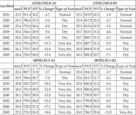
Table 11 shows the type of year projected every 10 years for the Guayalejo-Tamesí River Basin during the periods of 2010-2039 and 2040-2069, for models GFDLCM2.0 and MPIECH- 5, for scenarios A2 and B2, respectively, taking into account the P/T relation and the aforementioned criteria.
Considering the conditions detailed in Table 11, and regardless of the fact that through the WEAP program it is possible to get a wide variety of results concerning the supply/demand relation of the hydric resource in one region, this chapter makes specific reference to the unmet demands for water in the irrigation districts inside the Guayalejo-Tamesí River Basin.
Year/Mod GFDLCM2.0-A2 GFDLCM2.0-B2 meaT PCP P/T % Change* Type of Year meaT PCP P/T % Change* Type of Year
2010 25.2 811.4 32.2 -2.7 Normal 25.2 819.5 32.5 -1.8 Normal 2020 25.3 790.6 31.3 -5.4 Dry 25.4 817.2 32.2 -2.7 Normal 2030 25.4 773.0 30.4 -8.0 Dry 25.5 813.6 31.9 -3.6 Normal 2039 25.6 764.1 29.9 -9.6 Dry 25.7 810.1 31.6 -4.6 Normal 2040 25.6 763.2 29.8 -9.8 Dry 25.7 809.7 31.5 -4.7 Normal 2050 25.8 755.4 29.3 -11.5 Very dry 25.9 807.7 31.2 -5.5 Dry 2060 26.1 753.7 28.9 -12.6 Very dry 26.0 804.9 31.0 -6.4 Dry 2069 26.4 754.5 28.6 -13.4 Very dry 26.2 802.8 30.7 -7.1 Dry
MPIECH-5-A2 MPIECH-5-B2 meaT PCP P/T % Change Type of Year meaT PCP P/T % Change Type of Year
2010 25.4 807.7 31.9 -3.7 Normal 25.4 816.1 32.2 -2.7 Normal 2020 25.5 784.4 30.7 -7.0 Dry 25.6 811.7 31.7 -4.1 Normal 2030 25.8 763.7 29.7 -10.3 Very dry 25.8 806.0 31.2 -5.6 Dry 2039 26.0 751.9 28.9 -12.6 Very dry 26.0 800.6 30.8 -7.0 Dry 2040 26.1 750.7 28.8 -12.9 Very dry 26.1 799.9 30.7 -7.1 Dry 2050 26.4 739.5 28.0 -15.3 Very dry 26.3 795.8 30.3 -8.5 Dry 2060 26.8 734.3 27.4 -17.1 Very dry 26.5 790.8 29.8 -9.9 Dry 2069 27.2 731.9 26.9 -18.6 Very dry 26.8 786.7 29.4 -11.0 Very dry
*With respect to the current value of 33.06.
Table 11. Type of Year Projected, Models GFDLCM2.0 and MPIECH-5, Periods of 2010-2039 and 2040- 2069.
Table 12 summarizes the results for the demand for water that has been unmet annually in the irrigation districts (ID) inside the Guayalejo-Tamesí River Basin; it is expressed in millions of m3 and measured every ten years for the period of 2010-2069.
ID/Model of Climate Change Year
2010 2020 2030 2040 2050 2060 Total ID Xicoténcatl 029
GFDLCM2.0-A2 539.36 546.91 580.08 580.08 592.22 593.83 3,432.48 GFDLCM2.0-B2 539.36 539.36 539.36 539.36 563.63 580.08 3,301.15 MPIECH-5-A2 539.36 561.47 581.43 593.83 593.83 593.83 3,463.76 MPIECH-5-B2 539.36 539.36 555.54 580.08 580.08 580.08 3,374.50
ID/Model of Climate Change Year
2010 2020 2030 2040 2050 2060 Total ID Río Frío
GFDLCM2.0-A2 94.45 95.77 101.58 101.58 103.70 103.99 601.06 GFDLCM2.0-B2 94.45 94.45 94.45 94.45 98.70 101.58 578.06 MPIECH-5-A2 94.45 98.32 101.81 103.99 103.99 103.99 606.53 MPIECH-5-B2 94.45 94.45 97.28 101.58 101.58 101.58 590.90 ID San Lorenzo
GFDLCM2.0-A2 0.00 0.00 0.00 0.00 0.00 0.00 0.00
GFDLCM2.0-B2 0.00 0.00 0.00 0.00 0.00 0.00 0.00
MPIECH-5-A2 0.00 0.00 0.00 0.00 0.00 0.00 0.00
MPIECH-5-B2 0.00 0.00 0.00 0.00 0.00 0.00 0.00
ID 002 Mante M. Izquierda
GFDLCM2.0-A2 9.82 29.19 15.59 13.68 27.01 32.98 128.26 GFDLCM2.0-B2 9.82 28.79 14.49 12.72 25.71 32.22 123.74
MPIECH-5-A2 9.82 29.97 15.62 14.00 27.08 32.98 129.48
MPIECH-5-B2 9.82 28.79 14.93 13.68 26.46 32.22 125.88
ID 002 Mante M. Derecha
GFDLCM2.0-A2 15.10 40.96 24.92 21.67 37.03 45.27 184.95 GFDLCM2.0-B2 15.10 40.39 23.17 20.15 35.25 44.22 178.28
MPIECH-5-A2 15.10 42.05 24.98 22.18 37.14 45.27 186.72
MPIECH-5-B2 15.10 40.39 23.87 21.67 36.28 44.22 181.53
ID 1 Las Ánimas
GFDLCM2.0-A2 0.00 9.69 10.35 10.17 10.45 10.53 51.19
GFDLCM2.0-B2 0.00 9.56 9.62 9.45 9.95 10.29 48.87
MPIECH-5-A2 0.00 9.95 10.37 10.41 10.48 10.53 51.74
MPIECH-5-B2 0.00 9.56 9.91 10.17 10.24 10.29 50.16
ID 2 Las Ánimas
GFDLCM2.0-A2 0.00 11.61 12.39 12.17 12.52 12.61 61.29
GFDLCM2.0-B2 0.00 11.45 11.52 11.32 11.91 12.31 58.50
MPIECH-5-A2 0.00 11.91 12.41 12.46 12.55 12.61 61.95
MPIECH-5-B2 0.00 11.45 11.86 12.17 12.26 12.31 60.05
Table 12. Annual Demand for Water that Is Unmet in the Irrigation Districts inside the Guayalejo- Tamesí River Basin.
Based on these results, we can conclude that it is under the climate conditions obtained through model GFDLCM2.0-B2 where the coverage of the demand for water in the aforementioned river basin reaches the highest percentages; or, to put it differently, among the projected climate conditions to meet the demand for water in that basin, the least adverse correspond to those obtained by model GFDLCM2.0-B2. On the other hand, the most unfavorable projections about the same conditions correspond to model MPIECH-5-A2.
It is also noticeable that the most adverse conditions to meet that demand belong to the irrigation district Xicoténcatl 029; as a means to illustrate this, Figure 1 shows the projections on the unmet demand for the same district, according to the different models (million cubic meters [MCM] are used).
Year
MCM
Current
Figure 1. Unmet Demand for Water.
As this figure shows, scenario MPIECH-5-A2 presents the most unfavorable conditions and the fastest changes with regard to the unmet demand for water. On the other hand, scenarios B2 project less drastic changes with less immediate effects.
Given that model WEAP enables the user to incorporate a limitless series of scenarios within the calculus process, we decided to analyze several scenarios in which a number of changes are contemplated as adaptive measures to be possibly taken; the scenarios were:
Base scenario (BS): It deems it advisable to continue operating with the system of water rights and hydraulic infrastructure as it has been applied so far, overlooking any adaptive measure vis-à-vis climate change;
Irrigating-technification scenario (ITS): It values the gradual introduction of some kind of irrigating technification (by dripping, by aspersion, etc.) that leads to the optimization of the water volumes in concession for agricultural use;
Irrigating-technification scenario plus changing of the crops (ITS+CC): It entails the gradual introduction of irrigating technification plus a shift from having highly water- demanding crops to having moderate-demanding ones, such as Sorghum, Soy, Safflower or Grass species;
Irrigating-technification scenario plus a reduction of the cultivation areas (ITS+RCA): It poses the gradual introduction of the irrigating technification plus the gradual diminution of the cultivation areas to be irrigated.
Table 13 summarizes the results (expressed in percentages) concerning the average demand for water that is met monthly throughout the period in the irrigation districts, according to model MPIECH and scenario A2, and taking into account the adaptive measures that are proposed.
Irrigation Districts Scenarios
BS ITS ITS+CC ITS+RCA
Xicoténcatl 029 5.0 15.7 16.3 35.8
Río Frío 50.9 88.6 90.4 89.3
San Lorenzo 91.0 91.0 91.0 91.0
002 Mante Margen Izquierda 51.9 79.3 81.3 80.4
002 Mante Margen Derecha 41.1 57.1 58.3 63.2
Unidad de Riego 1 Las Ánimas 87.6 91.0 91.0 91.0 Unidad de Riego 2 Las Ánimas 87.6 91.0 91.0 91.0
BS=Base scenario, which includes the model’s projections about climate change; ITS=Irrigating-technification scenario;
ITS+CC= Irrigating-technification scenario plus changing of the crops; ITS+RCA= Irrigating-technification scenario plus a reduction of the cultivation areas.
Table 13. Results of the Adaptive Measures vis-à-vis Climate Change in the Irrigation Districts, Model MPIECH-5-A2.
It can be inferred from this information that the volumes of water in concession are higher than the natural offer of the hydric resource in the area under study. Such conclusion finds support in the fact that, even when the adaptive measures vis-à-vis climate change are considered, the levels of efficiency attained for the coverage of water demand keep being quite low indeed.
4.4. The effect of climate change on rainwater collection
As mentioned earlier, the two models that are most adverse for the main objective and purpose of capturing rainwater for irrigation would be the CCCMA-31 and the CSIRO-30, which can be observed in Figures 2 and 3, where the projections about precipitation according to different models and under scenarios A2 and B2 are presented.
400.0 450.0 500.0 550.0 600.0
UKHADGEM_A2 UKHADCM3_A2 MPIECH-5_A2 GFDLCM21_A2 MIROCMED_A2 W.A._A2 CSIRO-30_A2 CCCMA-31_A2
Year
Precipitation (mm)
Figure 2. Projections about Precipitation according to Different Models, Scenarios A2.
450.0 470.0 490.0 510.0 530.0 550.0 570.0 590.0
UKHADGEM_B2 UKHADCM3_B2 MPIECH-5_B2 GFDLCM21_B2 MIROCMED_B2 CSIRO-30_B2 CCCMA-31_B2 W.A._B2
Precipitation (mm)
Year
Figure 3. Projections about Precipitation according to Different Models, Scenarios B2.
Table 14 shows the findings of models CSIRO-30, CCCMA-31, UKHADGEM, and MPIECH- 5 under scenarios A2, which are the most negative for rainwater collection; the periodicity is of 10 years, with stations December, January, February (DJF), March, April, May (MAM), June, July, August (JJA), September, October, November (SON); likewise, the weighted average scenario is proposed (Table 15).
CCCMA-31_A2
Change (%) PCP (mm)£
Year/Station DJF MAM JJA SON DJF MAM JJA SON Annual 2020 -3.5 -3.2 -7.9 0.91 28.3 56.4 272.2 123.5 480.5 2030 -4.7 -4.7 -12.6 0.08 28.0 55.5 258.5 122.5 464.5 2040 -6.6 -6.6 -17.5 -0.65 27.5 54.4 243.9 121.6 447.4 2050 -6.3 -7.6 -22.4 -0.24 27.5 53.8 229.3 122.1 432.8 2060 -5.1 -8.4 -27.5 0.57 27.9 53.4 214.3 123.1 418.7 Weighted
Factor
1 2 4 3
CSIRO-30_A2
Change (%) PCP (mm)£
Year/Station DJF MAM JJA SON DJF MAM JJA SON Annual 2020 -3.9 2.5 -5.0 -1.8 28.2 59.7 280.7 120.2 488.8
2030 -5.1 3.6 -8.47 -3.9 27.9 60.3 270.8 117.6 476.6 2040 -7.2 4.6 -11.9 -6.0 27.3 60.9 260.5 115.1 463.7 2050 -7.0 6.6 -15.2 -7.1 27.3 62.1 250.5 113.8 453.7 2060 -6.1 9.1 -18.7 -7.8 27.6 63.5 240.2 112.8 444.2 Weighted
Factor
2 1 3 4
UKHADGEM_A2
Change (%) PCP (mm)£
Year/Station DJF MAM JJA SON DJF MAM JJA SON Annual 2020 -13.7 -3.6 -2.9 1.5 25.4 56.1 287.1 124.3 492.8 2030 -19.5 -5.3 -5.2 1.0 23.7 55.1 280.2 123.6 482.6 2040 -26.5 -7.4 -7.6 0.5 21.6 53.9 273.1 123.1 471.7 2050 -31.6 -8.6 -9.8 1.3 20.1 53.2 266.5 124.0 463.8 2060 -36.2 -9.6 -12.1 2.4 18.8 52.6 259.8 125.4 456.6 Weighted
Factor
4 3 2 2
MPIECH-5_A2
Change (%) PCP (mm)£
Year/Station DJF MAM JJA SON DJF MAM JJA SON Annual 2020 -5.7 -7.1 -0.7 4.9 27.7 54.1 293.5 128.4 503.6 2030 -7.8 -10.4 -2.1 5.8 27.1 52.2 289.5 129.6 498.3 2040 -10.7 -14.3 -3.4 7.1 26.2 49.9 285.6 131.1 492.9 2050 -11.5 -17.4 -4.4 9.6 26.0 48.1 282.5 134.2 490.8 2060 -11.6 -20.3 -5.5 12.7 26.0 46.4 279.4 137.9 489.8 Weighted
Factor
3 4 1 1
Table 14. Change of Stationary Front.
Weighted Average (WA)
Precipitation (mm) Reduction (mm)£
Year/Station DJF MAM JJA SON Anual DJF MAM JJA SON Total 2020 26.9 55.7 279.9 122.8 485.4 -2.4 -2.5 -15.7 0.4 -20.3 2030 26.0 54.5 269.6 121.5 471.6 -3.4 -3.7 -25.9 -0.9 -34.0 2040 24.7 53.1 258.9 120.2 457.0 -4.7 -5.1 -36.7 -2.2 -48.7 2050 24.1 52.2 248.5 120.4 445.0 -5.3 -6.1 -47.1 -2.1 -60.6 2060 23.6 51.4 237.7 120.9 433.6 -5.8 -6.8 -57.9 -1.5 -72.0
£With respect to the current values: 29.4 (DJF), 58.2 (MAM), 295.6 (JJA), 122.4 (SON), 505.6 (Annual).
Table 15. Change of Stationary Front, Weighted Average Scenario.
In this case the calculation of the weighted average was based on the station, according to the reduction attained by 2060; thus, for instance, for the DJF station the model that showed the highest reduction was the UKHADGEM-A2, so it was assigned the value of 4 (weighted factor), followed by models MPIECH-5-A2, CSIRO-30-A2, and CCCMA-31-A2, which were assigned the values of 3, 2, and 1, respectively. In this way, the weighted average scenario for the DJF station is built as follows:
WA(DJF) = (UKHADGEM-A2(DJF)*4 + MPIECH-5-A2(DFJ)*3 + CSIRO-30-A2(DFJ)*2 + CCCMA-31- A2(DJF)*1)/10
It is noticeable that in the calculus made for the weighted average the biggest reduction happens in summer (JJA), reaching a reduction of 19.6% as it goes from 295.6 mm (the current value) to 237.7 mm by 2060, i.e., 57.9 mm less in this station; by adding the reduction in all of the stations, we would get 72.0 mm, that is, 14.2% annually, which implies going from 505.6 mm at present to 433.6 mm by 2060.
After considering such amounts, it becomes manifest that there would have to be an annual reduction of 720 m3/ha or 7,200 m3 by 2060 in the project’s influential area which equaled 10 ha – a loss concentrated mainly in station JJA that would attain the value of 579 m3/ha, which would amount to a decrease in water availability of 5,790m3 or 5,790,000 lt in the project’s influential area.
In view of these results, it is recommended to put into effect and develop to a substantial degree programs of infrastructural design, integral management, and efficient use of hydric resources, together with the setting of appropriate calendars for irrigation that truly correspond to the species to be sown; the minimum and the maximum of available water, as well as the maximum reduction as projected by the climate change scenarios, must be taken into account. In other words, great attention should be paid to the results obtained in stations JJA and DJF, aside from assessing especially the scenario designated as the weighted average (Figure 4).
0.0 50.0 100.0 150.0 200.0 250.0 300.0
DJF MAM JJA SON
Actual PCP_2020 PCP_2030 PCP_2040 PCP_2050 PCP_2060
Precipitation (mm)
Season Current
Figure 4. Projection of Stationary Precipitation, Weighted Average Scenario.
Table 16 provides the monthly results found with the models that project more extreme changes; these values can also bring support to the programs of infrastructural design, integral management, and efficient use of hydric resources.
Month
Current Precipitation
(mm)
CCCMA-31-A2 CSIRO-30-A2
2030 2060 2030 2060
Change
(%) mm Change
(%) mm Change
(%) mm Change (%) mm January 13.3 -5.2 12.6 -2.2 13.0 19.6 15.9 49.8 20.0 February 6.2 -2.1 6.1 -4.8 5.9 -6.6 5.8 -14.2 5.4
March 6.9 -3.6 6.6 -11.3 6.1 0.3 6.9 -3.1 6.6
April 15.4 -24.3 11.6 -46.6 8.2 26.3 19.4 59.7 24.5
May 36.0 2.3 36.8 10.5 39.8 -6.4 33.7 -8.0 33.1
June 91.3 -14.4 78.1 -33.2 61.0 -25.8 67.7 -57.2 39.1
July 114.9 -4.1 110.2 -7.7 106.1 7.0 123.0 15.6 132.9 August 89.4 -18.4 72.9 -40.5 53.2 -1.3 88.3 -4.3 85.5 September 76.6 4.5 80.0 7.0 81.9 -5.5 72.4 -13.9 66.0
October 36.4 -20.8 28.8 -36.2 23.3 -11.1 32.4 -15.8 30.7 November 9.4 22.9 11.6 43.0 13.5 11.9 10.5 19.8 11.3
December 9.8 -4.7 9.4 -4.2 9.4 -17.3 8.1 -30.6 6.8 Annual
(mm) 505.6 464.9 421.3 484.2 461.9
Change
(mm) -40.7 -84.3 -21.5 -43.8
Change
(%) 8.1 16.7 4.2 8.7
Table 16. Change of Monthly Precipitation, Models CCCMA-31 and CSIRO-30, Scenario A2.
We can observe in this table that the months with a higher percentage of reduction are, in descending order, April, August, October, and June, respectively, for model CCCMA-31, scenario A2, both for 2030 and 2060, whereas for model CSIRO-30 the months with a higher reduction are, in descending order, June, December, October, and February, respectively.
As the monthly results show, the decrease in annual precipitation could be of 40.7 mm (8.1%) by 2030, according to model CCCMA-31-A2, and 21.5mm (4.2%) according to model CSIRO-30-A2; by 2060 the decrease would be between 84.3 mm (16.7%) and 43.8 mm (8.7%) for models CCCMA-31-A2 and CSIRO-30-A2, respectively.
It is opportune to mention that obtaining monthly averages or totals makes no sense, as the distribution of precipitation doesn’t follow a homogeneous pattern, i.e., the increase or decrease of 100% in a month with scarce precipitation may be insignificant, whereas the increase or decrease of 10% in a month with abounding precipitation can prove to be quite meaningful; thus, for instance, an increase or decrease of 50% in February and June,
according to the values of current precipitation presented in Table 16, would correspond to 3.1 mm and 57.45 mm, respectively, the first one of which may be taken it to be insignificant and the second as significant.
Due to the monthly analyses of the different models, it is highly likely that the uncertainty regarding the percentage of monthly variation in precipitation will grow, insofar as there will be few coincidences and a dearth of consistency as far as the deviations’ magnitude and direction are concerned; therefore, we can recommend too highly the utilization of the findings obtained through the analyses by station: Winter (DJF), Spring (MAM), Summer (JJA), and Autumn (SON) in the weighted average scenario, embodying as they do, worthy input for the task of planning all the aspects and analyzing all the variables required for the implementation of the project devoted to rainwater collection.
Aside from the changes in the average conditions, it is recommended to keep in mind the effects of extreme events, which seem to be steadily growing while their magnitude rises:
such happenings may well foster avenues that run counter to the aims of the project, causing damage in the infrastructure’s solidity and endurance as well as in the cultivation areas.
4.5. The effect of climate change on hydroelectric generation and the supply/Demand relation in the Sinú-Caribe River Basin in Colombia
The climatic-hydrological projections presented in Table 6 for the Sinú-Caribe River Basin point to certain changes and adverse effects on the volume that the Urrá1 Dam keeps in storage and, of course, on the generation of electric energy (Table 17, Figure 5a), as well as on the supply/demand relation of the whole basin.
By looking at the values of the first column (changes concerning the reference scenario), it becomes clear that all the models and scenarios indicate there is a reduction in the generation of electric energy that goes from 0.7% to 35.2%, while in the second column (changes concerning the maximum generation capacity) all the scenarios, including the reference scenario, indicate decreases with a range of 15.4% to 45.5%. The diminution in the Sinú River’s flow contribution to the Urrá 1 Reservoir is not only directly linked to the generation of electric energy (Figure 5a) but also to the volume kept in storage by the dam (Figure 5b).
On the other hand, taking into account the demand for the hydric resource in the domestic, industrial (agricultural and livestock), and commercial realms in 28 sites located inside the basin, we find that currently the required offer (190.1 MCM) is approximately equivalent to the supply delivered at present. However, as time goes on, all the scenarios project supplies lower than the required offer: at the end of the period of 2039 the delivered supply is to be between 402.3-619.4 MCM, depending on the climate scenario under analysis, with the weighted average pointing to a supply of 563.3 MCM (Figure 6); in the meantime, the requested offer reaches a value of 636.1 MCM, which suggests a strong pressure on the system and underscores the necessity of putting the hydric resources in the basin in order and under a sensible management.
Model/Variable
Electric
Generation Storage Vol. Flow Change₤
%
Change∞
%
Changea
%
Change_TMVb
% Change %
CCSRNIES-A21 -0.7 -16.5 -2.3 -12.9 -5.9
CSIROMK2B-A21 -11.3 -25.4 -1.9 -12.6 -2.3
CGCM2-A21 -0.8 -16.5 -6.9 -17.0 -11.8
CGCM2-A22 -13.7 -27.4 -7.8 -17.8 -13.3
CGCM2-A23 -13.4 -27.1 -6.4 -16.6 -11.3
HadCM3-A21 -35.2 -45.5 -29.7 -37.3 -34.9 HadCM3-A22 -25.9 -37.7 -20.1 -28.8 -23.8
HadCM3-A23 -2.9 -18.3 -10.5 -20.2 -14.2
Weighted
Average -18.8
Referenced or Current (Average Values)
0.0 -15.9
340.3 m3/s (in the dam) 527.7 m3/s (in all the
basin)
₤ Calculation made concerning what is designated as the Reference Scenario (1418.9 GWh/year), which would be the beginning or current scenario.
∞ Calculation made concerning the maximum generation capacity (1687.2 GWh/year).
aWith respect to the Reference Scenario, equal to 1,452.8 million cubic meters (MCM).
bWith respect to the TMV: Technology Maximum Value, equal to 1,630 million cubic meters (MCM).
Source: adapted from Ospina (2009)
Table 17. Changes in the Percentage of Electric Generation, the Storage Volume in the Dam, and the Flow.
Source: Adapted from Ospina (2009).
Figure 5. Reduction (expressed in %) for the Period of 2010-2039. a) Electric Generation. b) Storage Volume in the Dam.
Figure 6. The Demand for the Hydric Resource in the Basin: An Account of the Required Offer and the Delivered Supply.
Although the demand (540.7 to 2039 MCM) lies below the delivered supply (563.3 MCM), it is worth noticing that the requests posed by each one of the sectors and the 28 points in demand are not met in 100%, inasmuch as such appeals do not include losses in the systems, the reutilization of water in the processes or the management in the different petitionary locations, so the required offer (631.1 MCM) is much higher, as can be observed in that figure.
In this scenario the annual reduction of the average flow in the basin, as related to the present one, would be of 18.8%, as Table 17 shows – note that for this calculation there are underlying scenarios which estimate reductions as high as 35%, aside from the fact that for its analysis it only contemplates the period of 2010-2039, the estimates for the period of 2040- 2069 being more severe. Such reductions must be analyzed with great care, due to the implications they could have for the region in question, since reports from the Latin American Development Bank (Corporación Andina de Fomento [CAF, 2000]) indicate that in past events of what is designated as “El Niño” (1997-1998) the reductions in the flow of River Sinú have gone up to 33%, thus carrying deeply adverse consequences such as great losses in the agricultural production and other economic sectors, an increase in the demand for water and energy, the costs of resources for consumers, etc.
5. Participatory and adaptive approaches for water management
The effects of climate change on water resources are expected to bring multiple impacts over various sectors, whose consequences would be difficult to prevent completely and therefore to manage effectively. Therefore, from a policy perspective, policymakers are interested in identifying how to increase the capacity of organization and society to integrate uncertainty and complexity of climate change adaptation cross-sectorally. Along with water modeling tools and scenario development, described earlier in this chapter, there are other approaches to the management of water resources in situations of high uncertainty, involving adaptation and participation.
5.1. Participatory water management
Participatory water management is the involvement of stakeholders, who would not normally be involved, in different aspects of the management of their water resources. There are many different participatory methods that can be applied to increase such involvement (see Hare., et al, 2006). The participation of a wide range of stakeholders in management activities has been seen as important for supporting the assessment of situations of high uncertainty, from a cross-sectoral, integrated perspective (Rotmans, 1998). It has been promoted as a way of achieving societal acceptance of water management decisions (Mostert, 2003) which is of importance in those increasing cases where enhancing the capacity of local authorities, stakeholders, and interested groups to adopt and support approaches for implementing climate change actions is vital. The latter is becoming a critical policy issue (Brown., et al, 2010).
Participation is also being promoted actively for supporting the development of useful models and scenarios (Rotmans, 1998, Pahl-Wostl, 2002, Haag, 2001) used in resource management – for the purposes of increasing their degree of sectoral integration, quality, their validity, acceptance and use. This approach is called participatory modelling (see Hare (2011)) for an overview of the field within the water management sector). Participation is in addition viewed by researchers and policy makers as a means of bridging the policy- science-interface gap, leading to the improved use of research products in the management sector (e.g., Borowski and Hare (2007)). Those advocating a purely model-based approach to supporting adaptation in water resources management should take note of the considerable policy-science interface obstacles that exist to the water-sector adopting and using models for decision-making (see Borowski and Hare (2007), Mysiak., et al (2008), Webler., et al (2011)).
In Europe, the promotion of participatory water management is primarily driven by academia (see for example Ridder., et al (2005)) and a very favourable institutional enabling environment created by the EU Water Framework Directive (2000/60/EC; WFD). Article 14 (see EU (2002)) of the latter, prescribes minimum obligatory levels of stakeholder participation in the development of surface water quality management plans throughout the member countries of the union. It also seeks to encourage quite high levels of participation.
The levels of participation (see Mostert (2003)) range from low level participation involving simply informing stakeholders and consulting them on already designed plans, to actively involving them in planning and, at an even higher level, in decision-making. The WFD prescribes the first two and seeks to encourage the decision-makers to actively involve stakeholders in planning. Promoting participation in actual final decision-making is not considered by the WFD, and is not common in European water management.
The WFD and associated EU research projects developing experimental high-level participatory water management processes for it (e.g. EU FP7 NeWater project – (Moellenkamp., et al, 2010); EU FP7 AquaStress project – (Daniell., et al, 2010)) have provided a decade-long experiment in the potential uptake of participation as a serious tool of use in the water management sector. To date, the uptake of active forms of participation
(i.e. going beyond informing and consulting stakeholders) has been poor outside of research-driven processes, despite the institutional enabling environment of the WFD, and despite the financial and human resources being provided by the EU through the research sector to support this uptake. The reasons for this are manifold (see, for example, the TRUST project – (Krywkow., et al, 2007)). As Hare (2011) reports, there is often a lack of personnel, skills and organizational capacities to implement such active and intensive levels of participation with multiple stakeholder groups. The statutory and reward incentives of water management also often work against managers risking their reputations and perhaps jobs on developing participatory processes that might get out of control or slow down implementation of vital infrastructure projects, in cases where funding is time-dependent (op. cit). Videira., et al (2006) also suggest that the low level of prescribed participation in the WFD itself restricts the incentives for water managers to go beyond what is prescribed – why risk your job etc., when higher levels are not prescribed? Finally, as Borowski and Hare (2007) identified in their research – stakeholders - practitioners, policymakers and decision- makers - often do not have the time to participate in what will normally be time-intensive processes. If the water managers are not inclined to adopt high levels of participatory processes outside a research project, and stakeholders may often not have enough time, active, high levels of participation within the water management sector remains an aspiration.
This remains a critical problem for approaches to managing uncertainty in the face of climate change, such as adaptive management (Mysiak., et al, 2010) and adaptive governance (Huitema., et al, 2009) in which active stakeholder participation is a central component. Fortunately, as Hare (2011) suggests, these approaches, when considered from the perspective of niches, also contain a potential solution to the dilemma, which allows both adaptation and participation to be taken up and implemented. This solution will be returned to at the end of the chapter. First it is important to discuss adaptive management and adaptive governance and their role in managing water resources in times of climate change.
5.2. Adaptive management and adaptive governance
Previous experiences using a participatory water management approach keep being very valuable when trying to mainstreaming climate change adaptation into water resources management. Mainstreaming climate change adaptation is understood as a process of cross- sectoral integration of policy through common policy-making on adaptation which facilitate changes in socio-economic systems and governance regimes, aiming at dealing with uncertainty and capturing the opportunities for synergistic results in terms of increased adaptive capacity and lower vulnerability. However, in order to be able to continually maintain the experience needed to cope with uncertainty and change, the integration of actions and policies for water management needs to increase its own adaptive capacity, too.
Various experiences from the literature offer valuable examples on the way in which an adaptive approach has provided a systematic perspective that lead a management system to undertake the necessary adjustments in its structure, function, and performance under