207
The Effects of Global Shocks on Small Commodity-Exporting Economies:
Lessons from Canada
†By Valery Charnavoki and Juan J. Dolado*
We propose a structural dynamic factor model of a small commodity-exporting economy, using Canada as a representative case study. Combining large panel datasets of the global and domes- tic economies, sign restrictions are used to identify relevant demand and supply shocks that explain volatility in real commodity prices.
We quantify their dynamic effects on a wide variety of Canadian macro variables. We are able to reproduce all the main stylized fea- tures at business-cycle frequencies documented in the literature on this type of economies. These include a Dutch disease effect which has proven hard to find in empirical studies. (JEL E32, F14, F32, F43, F44, Q02, Q33)
A
s stressed by Kilian (2009), not all oil price shocks should be considered alike when assessing the implications of sudden changes in this price on the econ- omy. Fluctuations in the real price of oil may have very different dynamic effects on macroeconomic aggregates depending on their underlying sources (demand/supply, global/specific shocks). Moreover, it is essential to address the problem of reverse causality from these aggregates to the oil price in order to get correct estimates of the magnitude and persistence of these effects. Accordingly, a growing number of recent contributions to this literature have adopted structural VAR (SVAR) models to identify relevant shocks to the global crude oil market, including those coming from the global business cycle (see Kilian and Murphy 2012; Lippi and Nobili 2012). However, while most of these studies have focused on how different shocks impinge on oil-importing economies (especially on the US), much less attention has been devoted to analyze their effects on exporters of oil and other primary commodities.Our aim here is to fill this gap. Using a structural dynamic factor model frame- work, we investigate the effects (at business-cycle frequencies) of different global shocks driving real commodity prices (not all oil) on a large set of macro variables in a prototypical small commodity-exporting economy (henceforth SCEE). In
* Charnavoki: New Economic School, Nakhimovskii Prospekt 47, 117418, Moscow, Russia (e-mail: vchar- [email protected]); Dolado: Department of Economics Universidad Carlos III de Madrid and European University Institutes, Via della Piazzuola 43, 50133 Florence, Italy (e-mail: [email protected]).We are grateful to the three anonymous referees, José E. Boscá, Antonia Díaz, Lutz Kilian, Eva Ortega, Loris Rubini, and Ludo Visschers for helpful comments and suggestions. Financial support from the Spanish Ministerio de Educación (ECO2010-19357 grant), Comunidad de Madrid (Excelecon grant) and Bank of Spain (Excellence Programme grant) is gratefully acknowledged.
† Go to http://dx.doi.org/10.1257/mac.6.2.207 to visit the article page for additional materials and author disclosure statement(s) or to comment in the online discussion forum.
particular, our focus lies on the Canadian economy. The choice of this case study is dictated by the fact that Canada is a general commodity exporter, and not only an oil exporter, as well as by the availability of data on this economy, something which is not so common for other SCEEs. This facilitates carrying out our analysis in a data- rich environment where the effects and propagation mechanisms of the different shocks can be studied in a comprehensive way.
One convenient starting point for the rest of the paper is to briefly summarize the main predictions (hereafter denoted as features) which have been highlighted in the literature about the effects of these shocks on SCEEs:
• External balance effect, according to which trade and current account balances in SCEEs are usually positively correlated with their terms of trade (i.e., the ratio of export and import prices) and the world prices of exported commodi- ties in real terms. When real commodity prices go up, the revenue from exports exceeds the cost of imports, leading to an accumulation of foreign assets (or to a reduction of foreign debt). For the specific case of oil-exporting economies, Kilian, Rebucci, and Spatafora (2009) find that this effect is almost fully due to changes in the trade balance of primary commodities.
• Commodity currency effect, whereby real exchange rates in SCEEs are strongly correlated with commodity prices in real terms.1 Thus, as documented by Chen and Rogoff (2003) and Cashin, Céspedes, and Sahay (2004), an increase in real commodity prices results in an appreciation of the real exchange rate.
• spending effect, meaning that windfall income gains from commodity exports are partially spent inside SCEEs, driving up domestic demand. For example, Spatafora and Warner (1999) find in general a strong positive effect of the terms of trade shocks on all aggregate domestic spending components: consumption, investment and government expenditure.
• Dutch disease effect, whereby raising real commodity prices, again via an appreciation of the real exchange rate, lead to a fall in competitiveness and thus to a decrease in the output of the noncommodity tradable sectors in SCEEs, in contrast to the nontradable and commodity sectors where output grows (see Corden and Neary 1982).2 Despite its popularity, it is somewhat surprising that there is a striking lack of agreement on the relevance of this effect (see, e.g., Spatafora and Warner (1999) and Stijns (2003) for unfavorable and favorable evidence, respectively).3
Most of the empirical literature documenting these features suffers, however, from two limitations. First, in general, fluctuations in world commodity prices are treated as exogenously determined and reverse causality problems are ignored. Secondly,
1 Hereafter, real exchange rate is defined as a price of foreign consumption in terms of consumption in the domestic economy, i.e., rE rt = nE rt · p t∗ / pt, where nE rt is a nominal exchange rate in terms of domestic cur- rency per unit of foreign currency, p t∗ and pt are, respectively, foreign and domestic consumer price indices.
2 The terms ‘noncommodity tradable goods’ and ‘manufacturing goods’ are used interchangeably in this paper.
3 Notice that most of the literature on the Dutch disease has focused on its long-run effects rather than adopted a business cycle perspective, as we do here. Hence, a more accurate interpretation of this phenomenon in our setup would be an adjustment with Dutch-disease-like properties.
even in those studies where these problems have been properly addressed, the above- mentioned effects have been often analyzed separately rather than jointly.4 In view of these shortcomings, our goal is to use an empirical methodology that is free from these criticisms to check if it allows us to reproduce simultaneously all the previous effects in our representative SCEE, including the controversial Dutch disease effect.
As already mentioned, Canada becomes an attractive case study because its exports cover manufactured goods and a wide variety of primary commodities, not only energy resources, as has been the focus of the previous literature on this topic.
In effect, although energy products represent 23.5 percent of total merchandise exports in 2010, other basic products and materials related to agriculture sector, for- estry and mining account for about 40 percent of those exports. An additional advan- tage is the availability for this country of a fairly rich quarterly dataset covering a long period, 1975:I–2010:IV. Combining this information with other rich datasets capturing aggregate changes at the worldwide level which affect the performance of the Canadian economy is particularly useful to tackle the reverse causality problem.
In this respect, it is worth stressing that, despite the fact that the United States is the main trade partner of Canada, exclusive focus on the US economy, rather than on worldwide variables, may lead to misleading results when identifying shocks.
For instance, it may underestimate a global commodity demand shock, like the one starting from the late-1990s, which was driven to a large extent by developments in East and South Asia rather than in the United States.
Our proposed methodology combines two strands of the empirical literature deal- ing with large panel datasets. First, in line with Kilian (2009) and Kilian and Murphy (2012), we use the SVAR methodology to identify the main global shocks driving up the world commodity prices. More precisely, we consider three common factors that respectively explain the volatility of three large sets of macro variables at the worldwide level: global economic activity, global inflation, and a world commodity price index in real terms.5 Our benchmark identification scheme for these shocks relies on sign restrictions (combined with bounds on some elements of the impact matrix as in Kilian and Murphy 2012), supplemented for sensitivity purposes by a more conventional recursive scheme. Three main global shocks are identified dur- ing the sample period: (i) a global demand shock (GD), (ii) a global noncommodity supply shock (GS), and (iii) a global commodity-specific shock (GC).
Examples of positive and negative GD shocks include the global expansions and recessions that have taken place since the 1970s. Regarding GS shocks, the surge of information and communication technology innovations, productivity growth in emerg- ing economies or the deepening of trade liberalization in the 1990s could be associated
4 Examples are Kilian, Rebucci, and Spatafora (2009) and Jääskelä and Smith (2011) who use SVAR methodol- ogy and carefully designed measures of global activity to document, respectively, the external balance effect in a large set of fuel-exporting countries, and the commodity currency effect in the Australian economy.
5 Notice that the set of variables in our model differs slightly from that in Kilian (2009) and Kilian and Murphy (2012). Our model includes global inflation but lacks global commodity supply, given that supply data for many primary commodities are not so readily available as for the oil market. Thus, our GC shocks should be interpreted as accounting for both unexpected changes in the supply and demand of primary commodities which are orthogonal to the changes explained by the remaining two shocks. Yet, this is unlikely to be restrictive, since these authors find that the relative contribution of the oil supply shocks (including those originated in Canada) to fluctuations in real oil price is minor.
to positive (favorable) shocks whereas sudden increases in inflation expectations or natural disasters affecting noncommodity exporting countries provide examples of negative (unfavorable) shocks. Finally, negative GC shocks could be associated with increasing world commodity prices, whose origin can range from wars or natural disas- ters in commodity-producing countries to unexpected changes in precautionary demand for these commodities in fear of future supply shortages or to speculative trading.
Next, we analyze the propagation mechanisms of these shocks on the Canadian economy, allowing explicitly for dynamic interactions with the global economy in a data-rich environment. A natural empirical framework for this exercise is provided by structural dynamic factor models (SDFM)(Stock and Watson 2005; Forni et al.
2009) and factor-augmented VARs (FAVAR)(Bernanke and Boivin 2003; Bernanke, Boivin, and Eliasz 2005; Boivin and Giannoni 2009; Mumtaz and Surico 2009) esti- mated by modern Bayesian techniques. Both methodologies turn out to be rather convenient to analyze the effect of a small number of structural shocks on a large set of macroeconomic variables often exceeding the number of observations. Thus, in line with (Boivin and Giannoni 2009; Mumtaz and Surico 2009), we construct a recursive SDFM model containing two blocks of common factors: (i ) one corre- sponding to the global economy, and (ii) another pertaining to the SCEE economy.
Our main findings can be summarized as follows. First, we confirm the results obtained by Kilian (2009) and Kilian and Murphy (2012) about real commodity prices being driven by a variety of global shocks rather than by any specific one.
More specifically, we find that GD and GC shocks play a more important role than GS shocks in explaining the volatility of these prices. Secondly, focusing exclusively on these two shocks, we find that a rise in commodity prices generated by either a posi- tive GD shock or a negative GC shock generates a positive effect on external balances and commodity currency effects. The fact that the source of shocks does not matter for these two effects (features i and ii in the previous list) may explain why they have been found in standard reduced-form specifications where fluctuations in real commodity prices are assumed to be exogenous. However, regarding the other two effects (fea- tures iii and iv), we find that the source of the shocks matters a lot. For example, the manifestation of the Dutch disease effect at business cycle frequencies in the Canadian manufacturing sector is detected when the rise in the price of commodities is due to a negative GC shock. This is not the case under a positive GD shock which stimulates real output and real expenditures uniformly across industries and sectors. Given that GD shocks contribute significantly to explain commodity price volatility, this result illustrates why it is hard to detect such an effect when the source of shocks is ignored.
The rest of the paper is organized as follows. Section I presents the main features of our modeling approach for a SCEE, including the identification of the global shocks, a brief description of the data and the basics of the estimation strategy.
Section II reports the empirical results. In particular, using the dynamic responses of the global and Canadian economies to a positive GD shock and a negative GC shock, we illustrate the specific channels that give rise to the different stylized features in our specific SCEE. Section III provides a sensitivity analysis of our results regarding subsample estimation, alternative measure of global activity, etc. Finally, Section IV concludes. An appendix with two sections provides further explanations on our esti- mation and identification approaches.
I. A Structural Dynamic Factor Model
In this section we lay out the basics of our unifying empirical framework which allows for the identification of the main shocks driving the world commodity prices and for the analysis of their transmission mechanisms to our representative SCEE.
Our approach combines two strands of literature. The first one is related to the identification of the main underlying sources of shocks driving changes in com- modity prices, which so far has been mainly restricted to the global crude oil mar- ket (Kilian 2009; Lippi and Nobili 2012; Kilian and Murphy 2012). An important finding in this literature is that world commodity prices are driven by many shocks and their effects on the global economy can differ a lot. For example, both a global demand shock and an unanticipated disruption of oil supply generate an increase in oil prices. Yet, while the first shock stimulates global economic activity, the second shock reduces it. In other words, proper identification of the sources of changes in these prices is crucial for the analysis of their impact on the global economy and the formulation of appropriate policy responses.
The second one relates to the literature about SDFM (Stock and Watson 2005;
Forni et al. 2009) and factor-augmented VARs (FAVAR) (Bernanke and Boivin 2003; Bernanke, Boivin, and Eliasz 2005; Boivin and Giannoni 2009; Mumtaz and Surico 2009) which is useful to analyze the effect of a small number of structural shocks on a large set of macroeconomic variables.
A. Empirical Model
In line with Boivin and Giannoni (2009) and Mumtaz and Surico (2009), our model consists of two blocks. The first block corresponds to the global economy, while the second one summarizes specific detailed information about the SCEE. The state of the economy in these two regions is characterized by a small number K of unobserved factors, ( F t∗ ′, F t ′ ), where the vector with asterisks denotes three global factors, F t∗ = ( F Y,∗ t , F π∗ ,t , F C,∗ t )′ . Following Mumtaz and Surico (2009), global fac- tors are required to have an economic interpretation. Specifically, the first factor, F Y,∗ t , summarizes information about global economic activity and is extracted from a panel of international series, X Y,∗ t , characterizing global and regional output, indus- trial production and trade. The second factor, F π∗ ,t approximates global inflation and is extracted from international data on consumer/producer prices and GDP deflators, X π∗ ,t . Finally, the third factor, F C,∗ t , captures the development of real world commod- ity price index and is obtained from panel data on the price of a wide variety of primary commodities, X C,∗ t .6 The state of the SCEE is measured by a large set of macroeconomic and financial series for Canada, Xt , from which the K − 3 domes- tic factors, Ft, are extracted. Given that domestic factors are just used to provide a summary of the business cycle fluctuations in the large panel of Canadian economic variables, they do not require an economic interpretation.
6 The real world commodity price index estimated in this paper is more closely correlated with the measured export price index for primary commodities in Canada than with the real oil price. This is not surprising since, as explained above, Canada exports a wide range of commodities.
The different panel datasets and the factors are related in the following way:
(1) X∗ Y,t
=
Λ Y∗ 0 0 0 F ∗ Y,t +
e ∗ Y,t X∗ π,t 0 Λ π∗ 0 0 F ∗ π,t e ∗ π,t , X∗ C,t 0 0 Λ C∗ 0 F ∗ C,t e∗ C,t
Xt Λ Y Λ π Λ C Λ H Ft et
where X t∗ = ( X Y,∗′ t , X π∗′ ,t , X C,∗′ t )′ and Xt are data for the global and domestic econ- omies; F t∗ = ( F Y,∗ t , F π∗ ,t , F C,∗ t )′ and Ft denote the corresponding unobservable fac- tors; Λ i∗ and Λ j are loading matrices for global and domestic factors, respectively;
and e t∗ = ( e Y,∗′ t , e π∗′ ,t , e C,∗′ t )′ and et are zero-mean i.i.d. measurement errors which are assumed to be uncorrelated with the corresponding common components. Lastly, notice that the global factors are included explicitly into domestic block of the model as illustrated by the last row of (1).
Regarding the dynamics of the common factors, they are modeled as a restricted SVAR:
(2) F t∗
= Ψ 11(L) 0 F t∗ −1 + ut , Ft Ψ 21(L) Ψ 22(L) Ft−1
where Ψ ij(L) are lag polynomials of the finite order p, ut denote reduced-form resid- uals, such that ut ∼ n(0, Ω) and ut = A0 ϵ t, with structural shocks ϵ t ∼ n(0,I) and Ω = A0 A 0 ′ . Given the small size of the domestic economy, we impose the restric- tion that domestic factors have no effect on global factors.7 Moreover, it is assumed that global shocks are ordered first and that domestic structural shocks have no con- temporaneous effect on global factors. Hence, the right upper 3 × (K − 3) block of the matrix A0 is taken to be zero. Additional identifying restrictions on this matrix will be discussed further below.
B. Data
The database consists of a large balanced panel of quarterly data from 1975:I to 2010:IV which spans 281 series characterizing both the global and domestic economies. Those variables, which are nonstationary, are first differenced and all variables are demeaned and standardized prior to estimation. Further details about these series are provided in the online Appendix.
The foreign block includes data for the world economy (if available) as well as for the large regional blocks (Organisation for Economic Co-operation and Development,
7 Estimation of an unrestricted VAR model provides very similar dynamic responses of domestic variables to global shocks.
European Union, G7) and the United States.8 This block contains three large categories of variables, namely, real activity, inflation, and real commodity prices. Real activity is measured by real GDP, industrial production, volume of exports and imports, plus the index of global real economic activity constructed by Kilian (2009), which is based on representative freight rates for various bulk-dry cargoes.9 Global inflation summarizes data on implicit price deflators of GDP, consumer, and producer prices. Real commod- ity prices consist of a range of commodity price indices for energy, food, agricultural raw materials, base metals, and fertilizers collected by the World Bank.
The data for Canada contain many different real activity indicators, inflation series, exchange rates, and financial variables. In addition to these macro variables, a large number of disaggregated deflators and volume series for consumer expen- diture drawn from Canadian Socioeconomic Information Management (CANSIM) are included. Interestingly, we also extend this block of data by including sixteen relative indicators of Canadian aggregate expenditure, employment, and output vari- ables in relation to the corresponding indicators in the United States. The insight for using these relative indicators is to provide comparisons of the Canadian experience with that of a commodity-importing country, like the United States, for which one would not expect to observe symptoms of some of the previously listed features, notably the spending and Dutch disease effects.
Finally, to put the data into perspective, Table 1 summarizes the sectoral composition of the Canadian economy, whereas Table 2 illustrates its main business cycle statistics during the sample period. As shown in Table 1, although primary commodity sectors (agriculture, forestry, fishing, mining, and quarrying) represent only a small fraction of overall GDP (8.4 percent) and employment (5.5 percent), they have a disproportion- ately large effect on the Canadian trade balance. In particular, net exports of primary commodities represents on average 2.2 percent of GDP, whereas those of manufactur- ing goods and of services and utilities reach −2.4 and 0.8 percent of GDP, respectively.
With regard to Table 2, the main lesson to be drawn is that the business cycle statistics of the Canadian economy, though similar to those observed in the United States (e.g., Backus, Kehoe, and Kydland 1995; Schmitt-Grohé 1998), exhibit important differences, which are closely related to the effects of real commodity prices. In particular, the latter are positively correlated with trade balance and nega- tively correlated with the real exchange rate, illustrating somewhat the presence of external balances and commodity currency effects in the raw data. Yet, at first sight there is no sign of a Dutch disease since real commodity prices are positively correlated with real output in all sectors, including the tradable sectors (excluding commodities), like manufacturing. It is precisely for this reason the decomposition of the real commodity price changes into several structural shocks becomes key to
8 Unfortunately, quarterly GDP and industrial production data for BRIC countries are only available during the 1990s. However, our global block contains quarterly data on world exports and imports from the OECD database which captures the effect of growth in the BRIC economies on global economic activity since that decade.
9 The Kilian’s index of real activity as reported by Kilian (2009)(in percent deviations from linear trend) is signif- icantly more persistent than our (log) differenced series of world output and trade and, as a result, our global activity index has practically zero correlation with it. To make Kilian’s index comparable to ours, we transformed this index to log-deviations from trend as log(1 + x/100) and then computed the first differences of transformed series. Our global economic activity index has higher, but still very low correlation (equal to 0.07) with this transformed index.
ascertain whether this controversial feature remains absent once we account for the source of these innovations.
C. Estimation
Following Bernanke, Boivin, and Eliasz (2005), Boivin and Giannoni (2009) and Mumtaz and Surico (2009), the model is estimated using a two-step principal com- ponent analysis (PCA). In the first step, the largest PC are extracted from each of the panel datasets X Y,∗ t , X π∗ ,t , X C,∗ t and Xt to consistently estimate common factors driving the global and Canadian economies. In the second step, these factors are used for estimation of the restricted VAR in (2).10
10 We do not explicitly model an uncertainty in the measurement of factors, as in Bernanke, Boivin, and Eliasz (2005). The problem is that this procedure becomes extremely time consuming when sign identification is used
Table 2—Business Cycles in Canada: 1975:I–2010:IV
Cross-correlations with (leads/lags of) real commodity price
Volatility
Correlation with GDP
lags leads
−6 −1 0 1 6
GDP 1.48 1.00 −0.28 0.36 0.42 0.41 −0.01
primary commodity sector 2.37 0.48 −0.46 0.41 0.39 0.27 0.01
noncommodity tradable sector 4.06 0.91 −0.42 0.33 0.44 0.43 0.02
nontradable sector 1.10 0.85 −0.08 0.36 0.41 0.38 −0.09
Consumption 1.20 0.83 −0.12 0.28 0.37 0.39 −0.10
Investment 5.19 0.65 −0.03 0.41 0.40 0.29 −0.18
Employment 1.15 0.78 −0.06 0.45 0.45 0.37 −0.12
Government purchases 1.08 −0.09 0.01 −0.06 −0.09 −0.15 0.00
Net export (percent of GDP) 0.92 0.00 −0.12 0.29 0.39 0.35 0.03
Real exchange rate 4.03 0.12 −0.03 −0.03 −0.09 −0.13 0.33
Real commodity price 8.71 0.42 −0.19 0.74 1.00 0.74 −0.19
GDP in United States 1.42 0.80 −0.34 0.19 0.30 0.34 0.07
notes: Sample period is 1975:I–2010:IV; all variables except net export are in logarithms; all variables are filtered with HP-filter (λ = 1,600); primary commodity sector—agriculture, forestry and fishing, mining and quarrying;
noncommodity tradable sector—manufacturing; nontradable sector—utilities, construction, services.
source: CANSIM Canada, OECD
Table 1—Sectoral Composition of the Canadian Economy: Average Shares over 1975–2010
Value added (percent of total GDP)
Employment (percent of total
employment)
Export (percent of industry production)
Net export (percent of total GDP)
primary commodity sector 8.4 5.5 32.7 2.2
Agriculture, forestry and fishing 3.0 4.0 17.3 0.6
Mining and quarrying 5.4 1.5 45.1 1.6
noncommodity tradable sector 16.4 15.4 42.3 −2.4
Manufacturing 16.4 15.4 42.3 −2.4
nontradable sector 75.2 79.1 5.7 0.8
Utilities 3.1 0.9 6.0 0.2
Construction 6.1 6.0 — —
Services 66.0 72.2 6.9 0.6
note: Sample period is 1975–2010.
source: CANSIM Canada, annual
Note that, in the first step, we impose the constraint that global factors are included into the PC for domestic block of the model. So, if these global factors are really common components, they should be captured by the PC of Xt. To extract the remaining K − 3 domestic factors from the space spanned by the PC of Xt, we use the approach advocated by Boivin and Giannoni (2009). Accordingly, the follow- ing iterative procedure is adopted at the first step of the estimation. Starting from the initial estimates of the K − 3 principal components Ft of the domestic block of variables Xt, denoted by F t( 0), iteration proceeds through the following steps:
• Regress X t on F t( 0) and estimates of the global factors F Y, t* , F π* , t and F C,t * , to obtain Λ H(0 ), Λ Y(0 ), Λ π(0 ) and Λ C(0 )
• Compute ˜ X t( 0) = X t − Λ Y(0 ) F Y, t* − Λ π(0 ) F π* , t − Λ C(0 ) F C, t*
• Estimate F t( 1) as the first K − 3 principal components of X ˜ t( 0)
• Back to the Step 1. The algorithm is repeated until convergence in F t( j) is achieved.
On the basis of several information criteria for the choice of the number of fac- tors, we end up including 8 common factors for Canada. At any rate, the impulse response functions (IRFs) hardly change if additional domestic factors are consid- ered.11 This choice implies that the second step in our estimation procedure involves the estimation of a restricted VAR with 11 endogenous variables, namely 3 global and 8 domestic factors. The use of the AIC criterion indicates that two lags are enough to adequately capture its dynamics. Since this choice implies a large number of free parameters in the VAR system to be estimated with 144 observations for each variable, a Bayesian estimation procedure is used in this restricted VAR. Further details about the estimation procedure are provided in Appendix A.
D. identification of structural shocks
This section discusses the identification of the three global structural shocks:
(i) an unanticipated expansion of global demand (GD), ϵ D,∗ t , (ii) a global supply shock, unrelated to commodity markets (GS), ϵ s,∗ t , and (iii) a global commodity- specific shock (GC), ϵ C,∗ t . The last shock is aimed to catch unanticipated changes in the real commodity prices orthogonal to the first two innovations stemming from an unexpected contraction of the global commodity supply as well as by commodity-specific demand shocks, such as an increase in the precautionary demand on commodities.
The benchmark identification scheme for these global shocks is based on a mix- ture of sign and impact matrix restrictions, although we also provide results using a more conventional recursive ordering (see Kilian 2009), as a robustness check of
since it requires running the Kalman filter to draw the latent factors from their posterior distribution in each iteration of Gibbs sampler. Thus, this approach becomes unfeasible in practice.
11 Bai and Ng (2002) provide several criteria to determine the number of factors present in the dataset, Xt. Their panel information criteria i Cp1 and i Cp2 , for example, suggest the presence respectively of 8 and 7 factors in the panel for Canada. However, these criteria do not address directly the question of how many factors should be included in the VAR.
our results. Global factors are ordered first, implying that the rest of the world does not react instantaneously to domestic conditions in Canada.
sign restrictions Combined with short-run Elasticity Bounds.—In the bench- mark identification scheme, we impose sign restrictions on the IRFs of global fac- tors to global shocks. In particular, we assume that IRFs accumulated over four quarters should have the signs reported in Table 3.
These sign restrictions are imposed using the rotation procedure proposed by Rubio-Ramírez, Waggoner, and Zha (2010), as described in Appendix B.
Accordingly, a GD shock is associated with an increase in global activity, inflation, and real commodity prices. A negative GS shock implies a rise in inflation, and a fall in both real activity and real commodity prices. Finally, a negative GC shock results in increasing commodity prices, higher inflation and declining real activity.
A fundamental problem of the VAR model being identified through sign restric- tions is that, in contrast to the exactly-identified VAR, it does not provide a point estimate of the IRFs, which are only set identified. In other words, this implies that there is not a unique structural model characterized by the single impact matrix A0 , but a set of models (and a set of matrices 0 = { A0| A0 A 0 ′ = Ω}) that satisfy the identifying assumptions. This complicates interpretation of the results because medians (or other quantiles) of the IRFs computed for different time horizons often correspond to different structural models.
To alleviate this problem, we adopt the approach proposed by Kilian and Murphy (2012), where the set of admissible structural models is narrowed down by impos- ing bounds on some of the elements in the impact matrix A0 . In particular, these authors assume a very small short-run elasticity of oil prices to the oil supply as well as a small contemporaneous response of global real activity to oil-market spe- cific demand shocks. Accordingly, we impose here the additional restriction on A0 that the short-run elasticity of the real global activity to GC shocks is small.
Specifically, we assume that the corresponding element of the matrix A0 is in the range from −10 to 5 percent: −0.1 ≤ A0(1,2) ≤ 0.05 which, after proper scaling, corresponds roughly to the estimates of the short-run elasticity of the US GDP to real oil price reported in the literature (see, for example, Rotemberg and Woodford 1996; Hamilton 2008).12 Thus, only those structural models satisfying these sign and bound restrictions will be kept for constructing the reported IRFs in the sequel.
Following Kilian and Murphy (2012), these will be depicted as the area between
12 Mork, Olsen, and Mysen (1994), using data for 1967–1992, estimated real GDP responses to negative and positive oil price increases for the United States, Canada, Japan, Germany (West), France, the United Kingdom, and Norway. Estimated short-run elasticities for all these countries are small. Yet, for Japan, Germany and the United Kingdom, they are a bit higher than for the United States (one percent increase in oil price implies immediate fall of GDP by 0.022 percent in Japan, 0.036 percent in Germany, 0.047 percent in the United Kingdom and 0.015 percent in the United States).
Table 3—Sign Restrictions on Impulse Response Functions
GD Shock, ϵ D, t∗ GC Shock, ϵ C, t∗ GS Shock, ϵ s, t∗
Global economic activity, F Y, ∗ t + — —
Real commodity price, F C, ∗ t + + —
Global inflation, F π, t∗ + + +
the 16 percent and 84 percent quantiles of the posterior distribution.13 Notice that structural models with a very large negative value of A0(1,2) are associated with larger commodity price responses to GD shocks and smaller price responses to GC shocks. As a result, they may lead to counterintuitive results, like, e.g., that the oil crisis of 1979–1980 was mostly due to a positive GD shock rather than to a negative GC shock.14
recursive identification.—To check how sensitive are the results of our bench- mark scheme, an alternative scheme based upon recursive ordering is also consid- ered. In particular, as presented in Table 4, the impact matrix corresponding to the foreign 3 × 3 block is taken to be lower triangular. The global economic activity factor F Y,∗ t is ordered first, followed by the real commodity price index F C,∗ t and global inflation F π∗ ,t respectively. This ordering implies that the GS shock has no contemporaneous effect on both global economic activity and real commodity prices, while a GC shock is allowed to affect global inflation on impact since the definition of the latter includes changes of the commodity prices.
II. Empirical Results
This section presents the main empirical results obtained from our SDFM. First, we present the estimates of the three global factors, illustrate their dynamic response to the global shocks and show historical decompositions of these factors in terms of the shocks on the basis of the two above-mentioned identification schemes. Next, using Canadian data, we report the main dynamic effects of global shocks on this SCEE. In particular, given that a positive GD shock and negative GC shock turn out to be the more important ones in explaining the volatility of real commodity prices, for brevity we restrict our attention to the role of these two shocks in checking whether they can replicate for Canada the different effects listed in the introduction.15
13 Certainly the bounds in the area capturing the IRFs may mix the responses of different candidate models at dif- ferent horizons. Yet, given that their patterns are generally supported by the exactly-identified recursive scheme, we think that they provide a good illustration of the overall dynamics of the IRFs. Further, using 90 percent coverage areas instead of 68 percent ones does not imply any major change in the conclusions (see Charnavoki and Dolado 2012).
14 The models which allow for a strong negative impact effect of the GC shock on global economic activity, A0(1,2) < −0.1, result in less positive (more negative) response of Canadian expenditure and output variables to a negative GC shock, shifting downwards the IRFs to this GC shock. However, relative IRFs (in particular Canada versus US expenditures and sectoral output) are fairly robust to this impact restriction (see online Appendix). In fact, Dutch disease and spending effects become even more pronounced after a negative GC shock, but we do not still observe such effects after a GD shock.
15 IRFs for the individual domestic variables are generated by Gibbs sampling algorithm. For each iteration, we sequentially draw the variance-covariance matrix of measurement errors from the conditional inverse Gamma distribution, the non-zero elements of loading matrix from the conditional Normal distribution, and the parameters of the restricted VAR from the Normal-Wishart (see Appendix A). These realizations of the parameters are then
Table 4—Recursive Identification
GD Shock, ϵ D, t∗ GC Shock, ϵ C, t∗ GS Shock, ϵ s, t∗
Global economic activity, u Y, t∗ × 0 0
Real commodity price, u C, ∗ t × × 0
Global inflation, u π, ∗ t × × ×
A. Global Common Factors and shocks
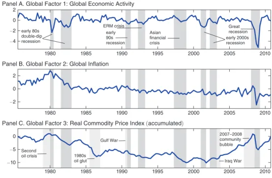
Figure 1 plots the estimated PC for the real activity, inflation, and real commod- ity prices datasets. These factors match closely the empirical evidence about interna- tional business cycles reported by Kose, Otrok, and Whiteman (2003) and Mumtaz and Surico (2009), as well as the main developments in the world commodity markets summarized by Kilian (2006) and Hamilton (2011) in their application to oil markets.
In particular, the global economic activity factor captures the main global down- turns between 1975:I and 2010:IV the double-dip recession at the beginning of the 1980s, the downturn in 1991–1993, the East Asian crisis in 1997–1998, the slowdown of the early 2000s after the Dot-com bubble collapse and 9/11 attacks, and finally the Great Recession of the late 2000s. Likewise, it captures the long expansion during the great moderation period. The real commodity price factor in turn reflects the most important events in commodity markets: the turbulence of the 1978–1981 period ignited by the Iranian revolution and outbreak of the Iran- Iraq war, the oil glut of the 1980s, falling commodity prices during the East Asian crisis in 1997–1998, rising commodity demand in 2000s, and the downturn in com- modity markets in 2008–2009. Lastly, the global inflation factor encompasses the stagflation of the 1970s-early 1980s, the rising food and energy prices in 2000s as well as the deflation of the late 2000s.
used to compute IRFs of the Canadian variables to structural shocks. The simulated data from each Gibbs iteration (after truncation of the first 10,000 realizations) are used to approximate the posterior distribution of these IRFs.
Figure 1. Principal Component Estimates of International Factors
note: Dark gray shaded regions represent the main global recessions; light gray shaded areas depict the main events in global commodities markets.
Panel A. Global Factor 1: Global Economic Activity
1980 1985 1990 1995 2000 2005 2010
−4
−2 0 2
Panel B. Global Factor 2: Global Inflation
1980 1985 1990 1995 2000 2005 2010
−2 0 2
1980 1985 1990 1995 2000 2005 2010
−10
−5 0
early 90s recession ERM crisis
Asian financial crisis early 80s
double-dip
recession early 2000s
recession Great recession
Panel C. Global Factor 3: Real Commodity Price Index (accumulated)
Second
oil crisis 1980s
oil glut Iraq War
2007−2008 community bubble Gulf War
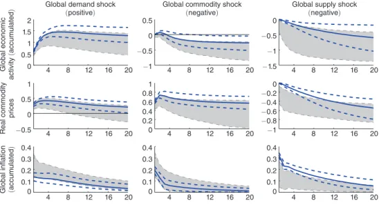
Figure 2 plots the IRFs of the factors to the three global shocks based on the sign restrictions scheme (shaded area covering the conventional 68 percent credible set reported in most of the literature) and the recursive identification scheme (solid line together with 68 percent interval). In general, both schemes provide similar results.
Thus, a positive GD shock generates a significant expansion in global economic activity, increases global inflation and pushes up real commodity prices, with the largest effect taking place within one year. A negative GS shock leads to a decline in real activity, accelerates inflation and depresses real commodity prices. Lastly, a negative GC shock gives rise to a temporary spike in global inflation and very strong increase in real commodity prices. As noticed earlier, the most important difference between the sign-restriction and recursive identification schemes is that, under the latter, the adverse effect of the GC shock on real activity is delayed for one year.16 By imposing a negative accumulated response of the real activity to a GC shock after four quarters, the sign identification scheme avoids this puzzling short-run phe- nomenon, which is also documented in Kilian (2009).
Figure 3 plots historical decompositions of the global economic activity, global inflation and real commodity prices based on the sign-identified structural model.
It shows the contribution of each of the three global shocks to the development of these global factors during the sample period. In this case, the results are virtually invariant to the method of identification. First, both schemes suggest that most of the volatility in the global real activity factor during this period has to be attributed
16 However, this delayed response of the real output to commodity shock conforms well to the results of Rotemberg and Woodford (1996) for the United States, which show that one percent increase in oil prices leads to a reduction in output of about 0.25 percent after five-seven quarters (with statistically significant decline only from the third quarter onwards).
Figure 2. Impulse Responses of International Factors to Global Shocks
note: Identification by sign restrictions—shaded area covering equally-tailed 68 percent credible set; recursive identification—median (solid line) together with equally-tailed 68 percent credible interval.
4 8 12 16 20
0 0.5 1 1.5 2
Global demand shock (positive)
Global economic activity (accumulated)
4 8 12 16 20
−1
−0.5 0 0.5
Global commodity shock (negative)
4 8 12 16 20
−1.5
−1
−0.5 0
Global supply shock (negative)
4 8 12 16 20
−0.5 0 0.5 1
Real commodity prices
4 8 12 16 20
0 0.2 0.4 0.6 0.8 1
4 8 12 16 20
−1
−0.8
−0.6−0.4
−0.2 0
4 8 12 16 20
0 0.1 0.2 0.3 0.4
Global inflation (accumulated)
4 8 12 16 20
0 0.1 0.2 0.3 0.4
4 8 12 16 20
0 0.1 0.2 0.3 0.4
to GD shocks, although a positive GS shock (possibly due to the raising productiv- ity in emerging economies and larger trade liberalization) also seems to play an increasing role from the mid-1990s. Further, some GC shocks seem to have contrib- uted to the economic slowdown at the beginning of the 1980s, as well as to revival of global economy after the Asian financial crisis during 1997–1998. Secondly, to some extent all three shocks played an important role in driving the global inflation.
While the episode of high inflation in the late 1970s-early 1980s is mostly attributed to the negative GS shock under recursive identification, sign restrictions point out to a combination of positive GD and negative GC shocks.
Finally, from the viewpoint of our subsequent analysis, the most interesting find- ing is that a large part of the volatility in real commodity prices during this period is mainly attributed to a GC shock and, to a lesser extent, to a GD shock.17 The former captures the disruption of the oil supply in the late 1970s–early 1980s, the oil glut of the mid-1980s, the region-specific downturn in 1997–1998 and the speculative episode in commodity prices at the beginning of 2008.18 The latter indicates that the Great Recession of the late 2000s was behind the falling commodity prices during
17 Though not reported, but available upon request, the (median) variance decompositions for the three global factors point out that the GC shock explains most of the volatility in the real commodity prices (about 80 percent in the recursive case and 60 percent in the model with sign restrictions), followed by the GD shock which accounts for approximately 20–25 percent. Hence, the GS shock explains practically nothing under the recursive identifica- tion scheme.
18 Since the East Asian financial crisis during 1997–1998 did not generate a strong global recession, our mea- sure of global economic activity fails to account for its effect on commodity markets. Moreover, the impact of this crisis was different across commodity groups. Oil prices recovered very quickly, and by the end of 1999 they reached their precrisis level. By contrast, prices of food, wood, base metals and fertilizers stagnated until the end of 2003. As a result, our measure of GC shocks differs slightly from the measure of oil-market specific demand shocks computed by Kilian (2009), especially after 1998.
1980 1985 1990 1995 2000 2005 2010
−10
−5 0 5 10
Global demand shock
Global economic activity (accumulated)
1980 1985 1990 1995 2000 2005 2010
−10
−5 0 5 10
Global commodity shock
1980 1985 1990 1995 2000 2005 2010
−10
−5 0 5 10
Global supply shock
1980 1985 1990 1995 2000 2005 2010
−6
−4
−2 0 2 4 6
Real commodity prices (accumulated)
1980 1985 1990 1995 2000 2005 2010
−6
−4
−2 0 2 4 6
1980 1985 1990 1995 2000 2005 2010
−6
−4
−2 0 2 4 6
1980 1985 1990 1995 2000 2005 2010
−2
−1 0 1 2
Global inflation
1980 1985 1990 1995 2000 2005 2010
−2
−1 0 1 2
1980 1985 1990 1995 2000 2005 2010
−2
−1 0 1 2
Figure 3. Historical Decompositions of the Global Factors: 1975:I–2010:IV note: Global factors—thick solid lines; identification by sign restrictions—shaded areas.
2008–2009. Hence, in the sequel, we will concentrate on these two shocks (a nega- tive GC shock and a positive GD shock) in analyzing their propagation mechanisms to the Canadian economy.19
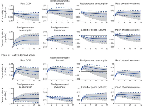
B. Transmission of international shocks to a sCEE
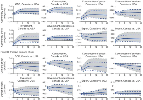
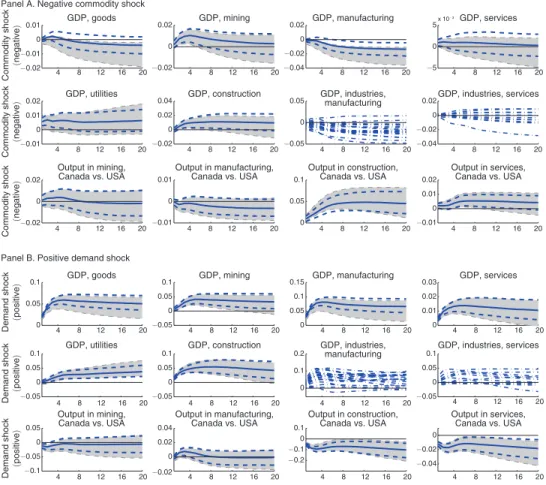
In this section we analyze the effects of these two shocks on the Canadian econ- omy at business-cycle frequencies. We divide our discussion into two parts. First, we illustrate that the sources of changes in real commodity prices are not specially important when studying external balances and commodity currency effects. Next, by contrast, we show that a negative GC shock and a positive GD shock imply very different effects on the aggregate expenditure components (spending effect) and sectoral output (Dutch disease effect) of the Canadian economy.
To report the IRFs of the Canadian variables, we convert them to the original units of the data using standard deviations computed in the first stage of the esti- mation procedure. Further, we standardize the shocks such that both the negative GC shock and the positive GD shock result in the same median level of increase in the real commodity price on impact. This level is chosen to be equal to one stan- dard deviation of the real commodity price factor, which roughly corresponds to an increase of 13 percent in the real energy price index. This procedure helps in making compatible the results on the conditional central tendency and the coverage areas.
Features for which the source of Commodity price Changes Does not Matter Much.—
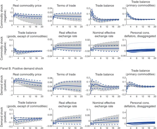
Terms of trade and external balances effects: We begin by reporting the results concerning terms of trade and external balances effects (feature I). Recall that this effect first predicts that a rise in commodity prices improves Canadian terms of trade. Secondly, when commodity prices are high (low), the current account and trade balances tend to improve (worsen). Since so far the evidence for this effect is restricted to oil-exporting economies (see Kilian, Rebucci, and Spatafora 2009), it is interesting to check its validity for other SCEEs.
Figure 4 plots the IRFs of the terms of trade and trade balances (as percent of GDP) to the two global shocks. Like in the graphs to be presented in the remaining subsections, the top panel A depicts IRFs of the relevant variables with respect to a negative GC shock, whereas the bottom panel B does the same for a positive GD shock. As can be observed, both shocks significantly increase real commodity prices and improve Canadian terms of trade. Their effects on external balances are however slightly different. While a negative GC shock improves the trade balance on impact, mainly through a sudden increase in the trade balance of primary commodities, a
19 A positive GS shock has a very similar effect to a positive GD shock on most of the Canadian variables under the sign identification scheme. Two differences worth mentioning are that: i) this shock has a deflationary effect on the nominal prices (in contrast to an inflationary effect of a positive GD shock), and ii) its effect is very persistent in contrast to GD shock which has a maximum impact in 1–2 years. Under the recursive scheme the effects of GS shock are mostly statistically insignificant.