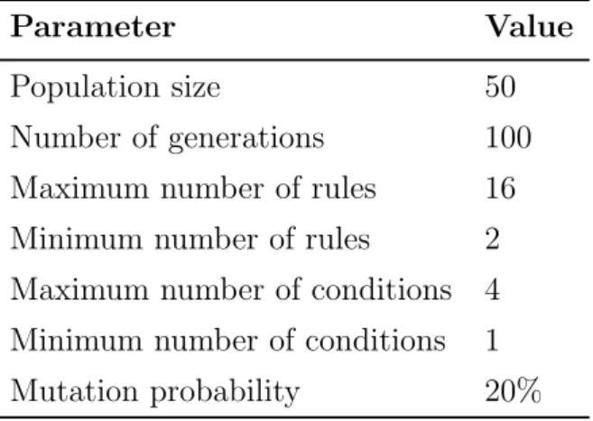
During each generation, the performance of the hyper-heuristic is calculated using a set of training data sets. For each of the text classification tasks there are different proposals that provide solutions.
Motivation
The AutoML works developed for the text classification task have allowed us to note that it is still necessary to develop a framework that has a more general process for selecting appropriate classification methods. Therefore, this thesis project aims to research the development of such a framework, including meta-features that allow a good representation of the data distribution of a dataset.
Objectives
Furthermore, for the algorithm to converge and find the best solution for such a data set, this optimization can be time-consuming if the search space is not bounded and also according to the data distribution of such a data set. In the case of the text classification task, there are proposals that show that the meta-characteristics of a data set provide very valuable information, which allowed them to develop works more focused on the stages before the selection of methods, as well the optimization for the acquisition of textual representations.
Literature Review
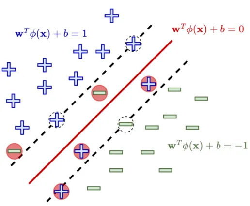
A meta-rule selects a method for a given dataset based on the evaluation of the meta-features extracted from that dataset. Such methodology serves as the basis for the development of the evolutionary model presented in this work.
Genetic Algorithms
- Basics
- Individuals
- Initial Population
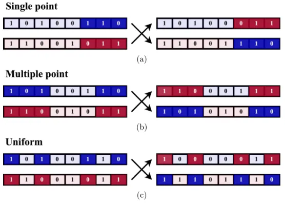
- Crossover
- Mutation
- Fitness
- Selection
- Termination Criterion
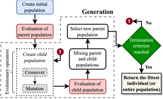
Similar to the crossover operator, the mutation operators are designed based on the representation of the individuals. Some methods directly select the best individuals from the child population as parents of the next generation.
Hyper-Heuristics
Selection Hyper-Heuristics
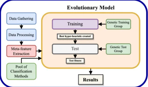
The training part contains the instances of the problem with which the individuals will be evaluated and developed during the evolutionary process. On the other hand, the instances of the test part are used to know the aptitude of the individuals to solve unseen instances of the problem.
Methods for Data Pre-Processing
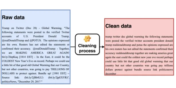
Cleaning Process
Stop words are a set of irrelevant words themselves, such as conjunctions, articles, prepositions and adverbs [52]. The NLTK (Natural Language Toolkit) library [53] provides access to more than 25 sets of stop words from different languages, which facilitates the process of removing them.
Transformation Process
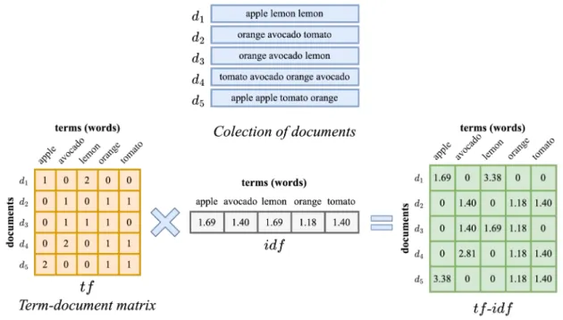
First, the term-document matrix is calculated using thetf(t, d) method, then a part of idf(t) is calculated in order to know the importance of a single term within the entire collection of documents. This results in an expression-document array, but now each element of the array represents a tf-idf value.
Normalization Process
The result can be represented as a diagonal matrix, where each element on the diagonal represents the importance of the expression. Within text classification, this procedure is applied to an expression-document matrix, where each row of the matrix is a vector, and the value associated with each column are the components of that vector.
Machine Learning and Deep Learning Meth- odsods
- Multinomial Na¨ıve Bayes
- Complement Na¨ıve Bayes
- Bernoulli Na¨ıve Bayes
- k -Nearest Neighbors
- Decision Tree
- Logistic Regression
- Support Vector Machines
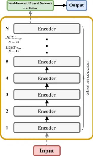
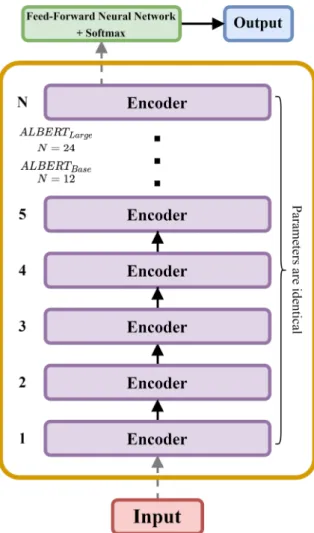
- BERT
- ALBERT
P (ci|x) determines the probability that sample x belongs to a class ci; P (xj|ci) is the probability that a feature xj occurs in a sample belonging to class ci; and P (ci) is the prior probability of the class ci. That is, a document is represented by a vector consisting of ones and zeros, where a 1 represents the presence of the feature in the document and a 0 represents its absence.

Evaluation Setup
Dataset Split
This allows to know a short estimate of how the classification method would perform when tested with real problems, using either of the two techniques (train-test, train-validation test). One of the most popular cross-validation methods isk-fold, this method divides the original data set intok subsets, of which k−1 are chosen to train a classification method, and the remaining subset to validate such a method. The performance of the classification method when using k-fold is the average of the sum of the performances obtained on each occasion.
Since it may happen that some of the generated subsets may not contain documents from any of the categories that appear in the original dataset. This problem can be avoided by applying stratification, which ensures that documents from all categories of the original dataset appear in each subset.
Evaluation Metrics
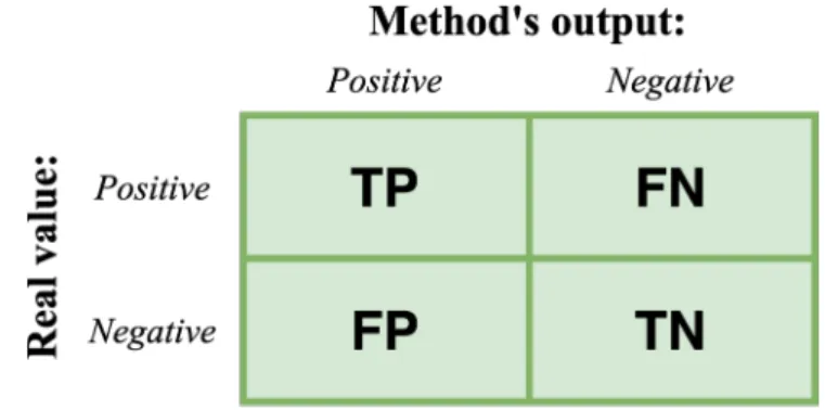
The value of k is defined by the user, and values such as 5, 10, or 20 are usually used. Accuracy is a metric that allows knowing the percentage of everything that is categorized as positive by the classification method that actually is (Eq. 2.20). And the Recall metric instead calculates from the total number of positive class documents how many hits the classification method had (Eq. 2.21).
Therefore, a high value of F1 means that Precision and Recall are high, and vice versa. In summary, the macroform calculates each metric for each class, that is, it creates a confusion matrix for each of the classes, and at the end it averages the obtained results.
Data Gathering
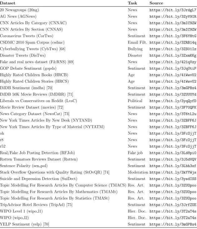
Dataset Description
50K Movie Reviews on IMDB (IMDBR) [71] Sentiment https://bit.ly/3ZUUUYd Liberals vs Conservatives on Reddit (LvsC) Politics https://bit.ly/3yqQyfD Movie Review Dataset (movies ) [72] Sentiment https://bit.ly/3F70QFK News Category Dataset (NewsCat) [73] News https://bit.ly/3T6tL2u New York Times Articles From the New Desk (NYTAND) News https://bit.ly/3ZBFF6J New York Times Articles By Material Type (NYTATM) News https://bit.ly/3ZBFF6J. Real/Fake Job Posting Detection (RFJob) Fake Job https://bit.ly/3Ld8pi0 Rotten Tomatoes Dataset Reviews (Rotten) Sentiment https://bit.ly/3J5dVQV. Stack Overflow Questions with Quality Assessment (StOvQR) [74] Moderationhttps://bit.ly/3kYYWjs Suicidality and Depression Detection Sentiment (SuiDect) https://bit.ly/3ysdISS Topic Modeling for Research Articles By Computer Science (TMACS) Res .
The data collected for this type of task comes from various sources such as Twitter, IMDB, Rotten Tomatoes, TripAdvisor and YELP. For the classification of research articles, the number of categories and documents is the same for the 3 data sets collected.
Data Processing
Within the entire group of datasets, SuiDect is the dataset with the largest number of documents (232,074), HCRS the smallest (430), wipo l2 is the dataset with the largest number of categories (922), while the smallest number of categories (2) can be found, among others, in different databases like csdmc, DisTws, imdbs. For each data set, a vocabulary is extracted from the training set and for each term in it the idf is calculated by Eq. Then, vectorization of each document in the training set is performed according to Eq.
2.1, allowing obtaining a matrix within which each element represents the importance of this term in the document. After vectorizing the training set, the resulting dictionary and idfs are reused to vectorize the test set using the same equalizer.
Classification Methods
Meta-Feature Extraction
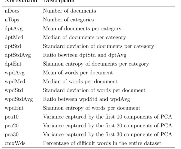
Similar to nDocs, nTops is the number of categories found in the training part of a dataset. This meta-attribute measures the centrality of the number of documents per category, but is sensitive to extreme values. A meta-feature that also measures the centrality of the number of documents per category, but is not sensitive to extreme values, is dptMed, which corresponds to the median of the documents per category.
Given the training portion of a data set, this meta-feature is calculated as the mean value of the ordered list of the number of documents that exist in each category. This meta-feature is the average size of the documents within a given dataset, with which we can generally identify how large or small the documents are.
Evolutionary Model
- Individuals
- Initialization
- Fitness Evaluation
- Crossover Operator
- Mutation Operator
- Selection
- Termination
- Evaluation of the Best Individual
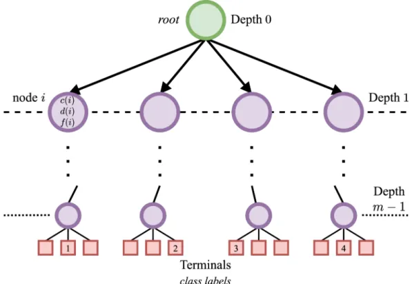
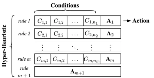
hh and meta-properties values are given to the EvaluateDataset function (shown in Algorithm 1), which is responsible for providing the action (classification method) to be applied to such a dataset. During the evolutionary process, the total fitness of a hh is determined using the genetic training set;. Due to the way the initial population and hhs generation is designed (see Algorithm 3), the size of the blocks/rules is not constant, so there can be blocks with few or many cells (multiple conditions).
Then select the rule for the second hh that is in the same position as the previously selected rule. The evaluation of hh on an unseen data set follows the same procedure as shown in Algorithm 1.
Analysis
Single Run
For a single run of the evolutionary model, the analysis focuses on visualizing the evolution behavior of hhs. With an analysis of this type, information can be obtained about the moment at which the population converges, that is, how the worst hh and the best hh have similar behavior. In some cases, this type of analysis is used to determine the number of generations in which a GA will work, because it can be used to see the moment at which the fitness of individuals does not reach improvements.
From these values, the maximum, average and minimum abilities of such a population in each of the generations are determined. In this way, the general behavior of the population in each generation can be analysed.
Multiple Runs
According to the method designed for the evolutionary process, hhs is evaluated for all populations after applying the evolutionary operators (except the initial population, which is evaluated at the beginning). With the calculation of the frequency of the actions, it is easy to determine which classification methods stand out the most, that is, if one approach is truly superior to another in certain data sets. For a total of executions of the evolutionary model, the frequency of the actions associated with the rules is obtained for each hh (rules without use are not intended).
Similarly, the frequency of occurrence of each of the 16 metafunctions in rules used by hhs is also calculated. Finally, each meta-attribute is calculated how often it is associated with each of the comparison operators (< and >).
Computational Time
Finally, the results of this hh are compared with the optimal one obtained by the best classification methods for each of the datasets in the group. This fitness is the average macro F1 value obtained for each of the genetic training group datasets. The multiple outliers of the box plot (found at the top) mean that there are very expensive methods within the pool, which correspond to instances of the SVM method when using different kernels (polynomial, sigmoid or radial basis function).
The behavior of hhs (in terms of fitness) during the evolutionary process corresponding to run 56 can be observed in fig. This optimal value is used to compare the performance of the final selected hh obtained using the same genetic test group. In this case, hh achieves a performance of 0.6805 by averaging the F1 macro values obtained in each of the datasets.
Similarly, these classification methods also appear as some of the optimal methods for the datasets of both genetic groups (training and testing).