Escuela Profesional de Ciencia de la Computación
“Improving the ILS-TQ technique for The High School Timetabling Problem”
Presentado por:
Jonathan Roger Alvarez Ponce
Para Optar por el Título Profesional de:
Licenciado en Ciencia de la Computación
Asesor: Dr. Alexander Javier Benavides Rojas
Arequipa, Agosto de 2019
profesores por haberme inculcado de los conocimientos necesarios, a mis amigos por haberme ayudado cuando lo nece- sitaba y a mi asesor por darme una buena orientaci´on.
HSTTP High School TimeTabling Problem
SA Simulated Annealing
LNS Large Neighborhood Search TS Tabu Search
GA Genetic Algorithm
VNS Variable Neighborhood Search VND Variable Neighborhood Descent ILS Iterated Local Search
HS Harmony Search
KHE Kingston High school timetabling Engine CSO Cat Swarm Optimization
RVNS Reduced Variable Neighborhood Search SVND Sequential Variable Neighborhood Descent SVNS Skewed Variable Neighborhood Search DGA Direct Genetic Algorithm
IGA Indirect Genetic Algorithm
ITC International Timetabling Competition GVNS General Variable Neighborhood Search PSO Particle Swarm Optimization
TQ Torque MT Matching
ILS-TQ Iterated Local Search - Torque 2TQ Two TQ moves
SC Random Swaps per Class CC Change Random Column S3R Swap Three Requirements ARD Average Relative Deviation SAI Simulated Annealing Inner SAO Simulated Annealing Outer
En primer lugar, deseo agradecer a Dios por haberme guiado a lo largo de estos cinco a˜nos de estudio y en todo lo que he realizado y realizar´e a lo largo de mi vida.
Asimismo, agradezco a mi familia que me ha apoyado en todo lo posible para forjarme como un profesional.
Tambi´en quiero agradecer a mi asesor Prof. Dr. Alexander Javier Benavides Rojas por haberme orientado correctamente para la realizaci´on de esta tesis, brind´andome lo nece- sario para no perderme en el camino.
Por ´ultimo, agradezco a la universidad, mi alma matter, por haberme brindado la for- maci´on que me permitir´a a mejorar la sociedad. Asimismo, agredecer a mis profesores que me han inculcado, tanto directa como indirectamente, de los conocimientos necesar- ios para ejercer mi profesi´on. Tambi´en agradezco al personal administrativo de la misma universidad por velar que todo est´e en orden.
El problema de planificaci´on de horarios para colegios de secundaria es un problema NP-Complete que consiste en asignar cursos, que son ense˜nados por profesores y asignados a cada clase, en periodos mientras se satisface restric- ciones. A trav´es de los tiempos, las meta-heur´ısticas han dado mejores resulta- dos para instancias reales de estos problemas que los m´etodos determin´ısticos ya que el espacio de b´usqueda de los problemas de planificaci´on son inmensos por lo que explorarlas todas resulta imposible. Mientras mejor sean los horar- ios, mayor es el rendimiento para los alumnos y profesores, adem´as que reducen los costos para generar estos horarios. Se proponen modificaciones, por sep- arado, a la b´usqueda local iterada (ILS) con el operador Torque (TQ) para las 34 instancias reales de colegios de Brazil. Estas modificaciones por sepa- rado cambian c´omo un horario es modificado y c´omo este horario es aceptado.
Nuestra implementation del esquema de enfriamiento del templado simulado, con algunas configuraciones de par´ametros, ha dado mejores resultados que nuestros otros m´etodos y soluciones m´as consistentes que el m´etodo original para algunas instancias. Adem´as, para crear otras instancias m´as f´acilmente, se ha creado un formulario.
Palabras clave: Colegios de secundaria, Problema de planificaci´on de horarios para colegios de secundaria, meta-heur´ısticas, B´usqueda Local Iterada, Operador Torque, creador de instancias.
The High School Timetabling Problem is an NP-Complete problem that con- sists in allocating subjects, that are taught by teachers and assigned to each class, to periods while satisfying constraints. Throughout the years, meta- heuristics haven given better results to real-life instances compared to deter- ministic methods since the search space for timetabling problems are huge and exploring it completely is impossible. The better the schedules are, the bet- ter the students and teachers’ performance, and the costs of generating these schedules are reduced. This proposal consists in modifications done separately to the Iterated Local Search (ILS) with the Torque (TQ) operator for the 34 real-life instances of schools of Brazil. These separate modifications change how a schedule is modified and how it is is accepted. Our Simulated Anneal- ing (SA) cooling scheme implementation, with some parameter tuning, gave better results than our other methods, and more consistent solutions than the original method for some instances. Furthermore, to create other instances more easily, a form was created.
Keywords: High school, High school timetabling problem, meta-heuristics, Iterated Local Search, Torque operator, instance creator.
1 High School Timetabling Problem 1
1.1 Constraints . . . 1
1.2 Timetabling Encoding . . . 2
1.3 Objective Function . . . 2
1.4 Final Consideration . . . 3
2 State of the Art 5 2.1 Iterated Local Search (ILS) . . . 5
2.2 Variable Neighborhood Search (VNS) . . . 6
2.3 Tabu Search (TS) . . . 7
2.4 Simulated Annealing (SA) . . . 7
2.5 Cat Swarm Optimization (CSO) . . . 8
2.6 Genetic Algorithms (GA) . . . 9
2.7 Hybrid Meta-heuristics . . . 10
2.8 Final Considerations . . . 13
3 Modified ILS-TQ 14 3.1 Input Encoding . . . 14
3.2 Constraint Violation Calculation . . . 15
3.3 Torque Operator (TQ) . . . 16
3.4 Constructive Algorithm . . . 16
3.5 Iterated Local Search . . . 18
3.6.1 Two ILS-TQ (2TQ) . . . 19
3.6.2 Relaxed Rule (RR) . . . 21
3.6.3 Random Swaps per Class (SC) . . . 21
3.6.4 Change Random Column (CC) . . . 22
3.6.5 Swap Three Requirements (S3R) . . . 22
3.6.6 Simulated Annealing (SA) Cooling Scheme . . . 23
3.7 HSTTP Instance Creator . . . 25
3.8 Final Considerations . . . 27
4 Tests and Results 28 4.1 Test Planning . . . 28
4.2 Instance Descriptions . . . 29
4.3 Results of the Original Method . . . 29
4.4 Results of our Implementation of the Original ILS-TQ . . . 32
4.5 Results of the Two ILS-TQ Moves (2TQ) Method . . . 34
4.6 Results of the Relaxed Rule (RR) . . . 37
4.7 Results of the Random Swaps per Class (SC) Method . . . 40
4.8 Results of the Change Random Column (CC) Method . . . 43
4.9 Results of the Swap Three Requirements (S3R) Method . . . 46
4.10 Results of the Simulated Annealing (SA) Cooling Scheme . . . 49
4.11 Best Result Comparison . . . 62
4.12 Schedule Improvement . . . 65
5 Concluding Remarks 77 5.1 Research Issues . . . 78
5.2 Future Work . . . 79
Bibliography 81
4.1 Instance features . . . 30
4.2 Original ILS-TQ implementation results . . . 31
4.3 Our ILS-TQ implementation results . . . 33
4.4 Our ILS-TQ implementation best results . . . 35
4.5 Two ILS-TQ results . . . 36
4.6 Two ILS-TQ best results . . . 38
4.7 Relaxed Rule results . . . 39
4.8 Relaxed Rule best results . . . 41
4.9 Random Swaps per Class results . . . 42
4.10 Random Swaps per Class best results . . . 44
4.11 Change Random Column results . . . 45
4.12 Change Random Column best results . . . 47
4.13 Swap Three Requirements results . . . 48
4.14 Swap Three Requirements best results . . . 50
4.15 Simulated Annealing Outer (SAO) cooling scheme placed at the end of each iteration with α parameters and t= 1 . . . 51
4.16 Simulated Annealing Inner (SAI) cooling scheme placed in the local search with α parameters and t= 1 . . . 52
4.17 SAI cooling scheme placed in the local search with α parameters and t = 100000 . . . 53
4.18 SAI results wheret = 1 andα = 0.5 . . . 55
4.19 SAI best results wheret= 1 and α= 0.5 . . . 57
4.21 Simulated Annealing (SA) best results where t = 100000, α = 0.5, and
t= 1 for feasible solutions . . . 60
4.22 SAI combined with Two TQ moves (2TQ) results wheret = 1 andα = 0.5 61 4.23 SAI combined with 2TQ best results wheret = 1 andα = 0.5 . . . 63
4.24 Method comparison . . . 64
4.25 Schedules generated by our ILS-TQ implementation . . . 67
4.26 Schedules generated by the method 2TQ . . . 68
4.27 Schedules generated by the method Relaxed Rule (RR) . . . 69
4.28 Schedules generated by the method Random Swaps per Class (SC) . . . . 70
4.29 Schedules generated by the method Change Random Column (CC) . . . . 71
4.30 Schedules generated by the method Swap Three Requirements (S3R) . . . 72
4.31 Schedules generated by the method SAI when α= 0.5 and t= 1 . . . 73
4.32 Schedules generated by the method SAI when α= 0.5 and t= 100000 . . . 75
4.33 Schedules generated by the hybrid method SAI with 2TQ . . . 76
3.1 Modification overview . . . 15
3.2 Torque operator example . . . 17
3.3 Two ILS-TQ example . . . 20
3.4 Relaxed Rule example . . . 21
3.5 Random Swaps per Class example . . . 22
3.6 Change Random Column example . . . 23
3.7 Swap Three Requirements example . . . 24
3.8 Simulated Annealing Inner overview . . . 25
3.9 Simulated Annealing Outer overview . . . 26
3.10 HSTTP instance creator user interface . . . 26
3.11 HSTTP instance creator XML output . . . 27
4.1 Best method vs. our ILS-TQ implementation graph . . . 66
Motivation and Context
Timetabling consists in assigning a set of activities to resources under complex constraints that vary depending of the problem context. It is an active area of research that has ap- plications on universities, traffic, schools, hospitals, sports, business, etc. Furthermore, this problem is NP-Complete which cannot be solved in polynomial time by deterministic algorithms.
TheHigh School TimeTabling Problem(HSTTP) is confronted in a lot of educational institutes worldwide. It consists in assigning resources such as teachers, and students in different time slots that represent lessons. However, this assignment has to satisfy a num- ber of constraints such as avoiding the same teachers or students assist two lectures at the same time. The objective of this problem is to get a schedule that minimizes these conflicts.
These conflicts are divided into hard constraints, and soft constraints: the former must be satisfied since it represents the feasibility of the solution, whereas the latter rep- resent preferences, and some of them might not be satisfied. A schedule is better if it violates less soft constraints.
Since there are many high schools, they might have different constraints, and some of them might be harder to satisfy. However, we assume that the corresponding high schools have already defined their constraints, and they have also defined which students attend which lessons, and the teachers who teach them. Furthermore, out of all these approaches, the one provided by Saviniec and Constantino (2017) has been selected to be improved since we believe we can improve it by setting a better perturbation operator.
There are no deterministic algorithms that can solve NP-Complete problems in polynomial time. However, according to Templatetypedef (2014), other kind of solutions can be applied such as: approximation algorithms, pseudopolynominal-time algorithms, randomized algorithms, parametrized algorithms, fast exponential-time algorithms and heuristics. The last ones are divided in heuristics, meta-heuristics, and hyper-heuristics, and, these last two have showed to solve these kind of problems efficiently. Furthermore,
gorithms have been chosen to be implemented since hyper-heuristics just use a group of meta-heuristics, and they cannot be used if there are no meta-heuristics implemented be- forehand. Moreover, hyper-heuristics’ difficulty is just about tuning how often they will use meta-heuristics to solve a problem, and it is not the implementation itself (Herbawi, 2014).
From my point of view, better solutions to this problem will result in better high school schedules. Therefore, students’ performance will increase, and this increased per- formance will help them perform better in college and other aspects of life.
Problem Statement
The problem being solved is the High School Timetabling Problem (HSTTP): given a set of requirements that provides information about the structure of each lesson, and a set of constraints with their respective weights, a feasible schedule that violates the least constraints is generated.
Objectives
To propose methods based on the Iterated Local Search - Torque (ILS-TQ) technique to solve the HSTTP.
Specific Objectives
• To research recent techniques in solving the HSTTP.
• To understand their operators, and how they modify their solutions.
• To implement the ILS-TQ technique by Saviniec and Constantino (2017).
• To propose methods to improve the ILS-TQ.
• To implement a form to create other instances to this problem for our methods.
• To compare results to the original ILS-TQ technique.
Thesis Organization
This work is organized as follows:
In Chapter 2 the state of the art of methods that try to solve variations of the HSTTP is given. These methods are focused on meta-heuristics.
In Chapter 3 the methods proposed to improve the ILS-TQ are explained in detail.
Additional to our proposal, a form to create instances to this problem is shown too. At the end of this chapter, there is a section focused on explaining the difference between the original method, and ours.
In Chapter 4, all the results obtained by our methods are shown, they are also compared with the original method. At the end of this chapter, in order to compare how each method’s schedules change over time, schedules given by these methods at the 10th, 50th, 100th and final iteration are shown.
Chapter 1
High School Timetabling Problem
The High School Timetabling Problem (HSTTP) consists in efficient assignation of two resources: teachers and classrooms through time. This assignment problem is more diffi- cult due to some constraints such as teachers’ preferences for scheduling and classrooms’
availability.
The HSTTP that is being solved is the same as the problem by Saviniec and Con- stantino (2017) which only consists of five hard constraints, and three soft constraints, these hard constraints represent the feasibility of the solution (i.e. determines whether the schedule is impossible due to having the same teacher teach two classes at the same time), whereas the soft constrains represent the quality of the solution (i.e. the schedule is possible, but might be more or less preferable). Requirements, and teacher unavailable periods are represented by tuples. The following subsections explain these variables in more detail, but this explanation is very similar to the one by Saviniec and Constantino (2017) since it is the same problem.
1.1 Constraints
They also take the following constraints into consideration:
• Hard constraints: they represent the feasibility of the solution.
– hc1: each requirement must be assigned to exactly θ times a week.
– hc2: a class must attend exactly one meeting per period.
– hc3: a teacher must teach at most one lesson per period.
– hc4: teachers must not be assigned periods in which they are unavailable.
– hc5: each requirement must have less or equal thanγ assignments per day.
• Soft constraints: they represent the quality of the solution.
– sc1: each requirement should have at least µdouble lessons a week.
– sc2: idle periods in the schedule of teachers should be avoided.
– sc3: the teachers’ schedules should be concentrated on a minimum number of days.
1.2 Timetabling Encoding
The input data to construct a timetable is given by two parameters:
• R: a set of tuples (c∈C, t∈T, θ∈N, γ ∈N, µ∈N) in which the subject of a class c is taught by a teacher t, and that subject has a duration of θ timeslots at most γ times per day. Also, that subject has a minimum number of weekly double lessons µ.
• U: teacher’s unavailable periods are represented by a tuple u ∈ U in the format (t∈T, d∈D, h∈H) in which teacher t is unavailable at period h of day d.
The set of timeslots will be defined by P as (d, h) ∈ D×H where d is day, and h is hour. Timetables are represented by a 2D array Z in which the rows represent classes, and the columns represent timeslots. Each array’s cell Zej points to a requirement tuple r ∈R assigned to class c∈C in timeslot j ∈P.
1.3 Objective Function
The objective function indicates how good a solution is, and it takes into consideration all soft constraints, and hard constraints, except for the first two of the latter since they are always satisfied.
Let βihc, and βisc be the number of times that constraint types hci(i = 3,4,5), and sci(i = 1,2,3) are violated, and let αhci , and αisc be the penalty constants associated to their respective violations to penalize them. Therefore, the objective function minimizes the following weighted sum:
minf(Z) =
5
X
i=3
αhci ·βihc+
3
X
i=1
αisc·βisc (1.1)
The first term of (1.1) measures the feasibility of the solution which is represented by all the hard constraint violations whereas the second term measures the quality of the solution which is represented by all the soft constraint violations. Since the feasibility of the solution is more important than the quality of it, then all values of αihc must be
greater than αsci to ensure that hard constraints are satisfied.
The values of βihc, andβisc are computed as follows:
β3hc = P
t∈T
P|P|
j=1(πij −1),∀(πij > 1), where πij is the number of times teacher t has been assigned to a timeslot j.
β4hc=P
t∈T
P|P|
j=1ρij, whereρij = 1 if teachertis assigned to teach at an unavailable timeslot j.
β5hc=P|R|
r=1
P
d∈D(σrd−γr),∀(σrd> γr), whereσrd is the number of times ther−th requirement has been assigned in a day, whereas γr is the maximum number of daily meetings.
β1sc =P|R|
r=1(µr−φr),∀(µr > φr), whereµr is the minimum number of double lessons for the r−th requirement, andφr is the total number effectively scheduled.
β2sc =P
t∈T
P
d∈Dηtd, whereηtd is the number of idle periods occur in the schedule of teacher t on day d.
β3sc =P
t∈T xt, wherext is the number of working days are scheduled to teacher t.
In their implementation, they used the following values for the corresponding penal- ties: αhc3 = 100.000, α4hc= 100.000, αhc5 = 10.000, α1sc = 1, αsc2 = 3, and αsc3 = 9
1.4 Final Consideration
The HSTTP problem we are aiming to solve has many variables such as constraints, classes, days, periods, requirements that must be taken into consideration in order to get a high quality schedule. However, this cannot be done with an exact method since there are many possibilities to build a schedule. There areq requirements that must be filled in d×tperiods where dis the number of days, andtis the number of timeslots for each day, and each requirement can appear more than once. So, there are: (d × t)! permutations of these requirements for one class, and since there are c classes, it becomes: (d × t)!c possible schedules that must be checked. Each schedule must be checked in order to know how good of a solution it is. Each objective function iterates over (d × t) × c elements per schedule, so, its computational complexity is:
O(((d × t)!c) × ((d × t) × c)) (1.2)
For example, the smallest instance in our dataset has 4 classes, 5 days, and 5 times- lots, so there are: 100 × (25!4) different ways to form a schedule. 25! is approximately 1025 so (25!)4 is approximately 10100. Thus, there are roughly 10102 different schedules.
A computer that does 109 operations per second would take 3 × 1085 years to compute all schedules. This shows that exact methods cannot be applied to these problems, so, meta-heuristics must be used in order to find feasible solutions in a reasonable time that is generally 10 minutes up to a day.
When the solution space is too large, exact methods cannot find the optimum solu- tion in a reasonable time, so, meta-heuristics are generally used to find a near-optimum solution. In the next section, some methods that apply meta-heuristics to solve this problem are explored.
Chapter 2
State of the Art
The HSTTP has been studied for many years, and many solutions to its variations have been proposed throughout the years. However, since it has been proven to be an NP- Complete problem, exact solutions cannot be applied to real life high schools. Therefore, meta-heuristics have been used to solve bigger, and more complex instances. One problem with these techniques is that they cannot always be compared since they might generate a schedule for a specific school. The Kingston High school timetabling Engine (KHE) by Kingston (2015), which is an open-source ANSI C library which provides a fast, and robust foundation for solving problem instances related to the high school timetabling problem, is often used by some authors such as Brito, Fonseca, Toffolo, Haroldo, and Marcone (2012); Demirovi´c and Musliu (2017); Fonseca and Santos (2014); Fonseca, Santos, and Carrano (2016); Fonseca, Santos, Toffolo, Brito, and Souza (2012, 2016); Yousef, Khader, Kheiri, and Ozcan (2013) to generate initial solutions. Meta-heuristics are methods used to find near-optimal solutions by perturbing a solution or group of solutions and storing the best found so far.
2.1 Iterated Local Search (ILS)
Gendreau and Potvin (2005) explain that Iterated Local Search (ILS) is a meta-heuristic that starts with a basic solution, and then finds the local optimum based on that solution.
In order to escape this local optimum, it applies a perturbation operator to the solution, and then finds the local optimum of that solution.
Saviniec and Constantino (2017) propose a simple, yet efficient algorithm which is the classic ILS meta-heuristic but with a perturbation operator called Torque (TQ). It surpasses the results of Fonseca, Santos, Toffolo, et al. (2016) in almost all problem in- stances. They also propose another perturbation operator called Matching (MT) without significant improvements. It is similar to their earlier work by Saviniec, Aparecido, and Romao (2013), but with a different local search.
Their TQ operator constructs a graph by choosing two periodsti, tj. Each vertex in
the graph represents the pair (ti, tj) for each class, and they are connected if, and only if there is a teacher clash by swapping the pair of one vertex. The generated graph consists of one or more connected components, and each TQ move consists in swapping all the pair for each vertex that belongs to a component. Thus, a new schedule is generated.
The perturbation operator is a single TQ move where ti, tj, and the component to be swapped are chosen randomly. Their local search is done by iterating through all possible timeslot pairs, and for each pair, they generate its corresponding graph. Each of its components are swapped generating new solutions. If the new solution improves the current one, then former replaces the latter, and the remaining components are swapped.
This process is repeated until there is no further improvement. At the end of the local search, the local optimum is returned. The new local optimum is compared with the best solution so far, and replaces it if it is better. If three local optimum cannot improve the best solution so far, the current solution is reset to the best solution so far. The stopping criterion is a time limit of ten minutes.
2.2 Variable Neighborhood Search (VNS)
The main characteristic of the Variable Neighborhood Search (VNS) is that it considers a number of neighborhoods to be explored, and each one is explored according to its suc- cess: if there is no better solution, then the next neighborhood is explored. If a better solution is found, it goes back to the first neighborhood Gendreau and Potvin (2005). A neighborhood is formed by all solutions that can be reached with a certain operator, and the closest neighborhood of a solution is made by all the solutions that can be reached by applying an operator once to that solution.
Saviniec and Constantino (2017) also propose a VNS which uses the MT, and TQ operators. However, no significant improvement was done compared to their ILS Imple- mentation. The most important part of their implementation are both operators. The MT operator selects a set of requirements of the same class, builds an N×N cost matrix where N is the number of requirements with their respective timeslots, and each cell is filled with the cost of inserting the requirementiin the timeslotj. This cost matrix is used to solve the corresponding assignment problem by applying the primal–dual algorithm by Carpaneto and Toth (1987). The solution of the assignment problem is the permutation that minimizes the objective function.
The VNS-HS by Fonseca and Santos (2014) starts by using the KHE, and then applies the VNS with improvements on some instances. They compare some variants of this meta-heuristic: The Reduced Variable Neighborhood Search (RVNS) has no descent phase, therefore improving its computation time when the neighborhood structure is ex- tensive; the Sequential Variable Neighborhood Descent (SVND) only explores the k−th neighborhood at each iteration k; and the Skewed Variable Neighborhood Search (SVNS) also accepts worse candidate solutions by following a relaxed rule, that calculates the distance between the candidate solution, and the best solution so far, and that considers one neighborhood structure in each iteration. Since the last variation gives better results
compared to the other two variations, some relaxed rules might improve Saviniec et al.’s Saviniec and Constantino (2017) method.
2.3 Tabu Search (TS)
Tabu Search (TS) is a meta-heuristic that moves from the current solution to the best neighbor that is not in the tabu list. This is used to avoid cycling moves Glover (1989).
The TS by Minh, Thanh, Trang, and Hue (2010) builds an initial solution with a greedy algorithm that splits each course in blocks (i.e. consecutive lectures) to be assigned on consecutive periods. Each course is split in different combinations of blocks (i.e. block splitting way) according to the constraints, then it calculates all period-assigning ways for each block for each course. After that, it selects the block-splitting way that has the block that belongs to the course with the smallest number of possible period-assigning ways to be placed in a period-assigning way. That causes the least reduction of those period-assigning ways. Their initial solution is improved with TS primarily by using single moves. It also applies swap moves, and block-changing moves when there is no improvement with single moves. There are two tabu lists: one for single moves, and another one for block-changing moves. They applied their algorithm to three real-world instances of two high schools of Vietnam, but there are no comparison with standard benchmarks. The initial solution constructive heuristic is more expensive than Saviniec and Constantino (2017) greedy algorithm, but it might provide a better initial solution.
2.4 Simulated Annealing (SA)
Simulated Annealing (SA) is a meta-heuristic that tries to find the global optimum in a large search space (Du & Swamy, 2016). It starts with an initial temperature which de- creases with each iteration by a factor ofα, and solutions that are worse may be accepted according to the current temperature, and the difference between the current solution, and the best one.
Zhang, Liu, M’Hallah, and Leung (2010) propose a SA to generate their initial so- lution, and another one to improve the initial solution. The first SA that they use selects a period that causes conflict in any day to exchange it with another random period for a random permutation of classes. It updates the best solution so far if the swap neighbor improves it. Their second SA generates a random permutation of periods where the first one is selected, and swapped with the rest of the periods in the permutation for each ran- dom class. It updates the best solution so far if the swap neighbor improves it, and it does not violate any hard constraints. They have two groups of datasets: the hdtt4-hdtt8, and from Greek schools. A modification to its local search might be used as a perturbation phase since it is not as expensive as Minh et al. (2010).
The SA proposed by Demirovic and Musliu (2017) uses a bitvector representation to improve an initial solution generated with the Kingston High school timetabling Engine (KHE). For each lesson, it creates 2 +m of vectors of length n where m is the number of different durations each sub-lesson has, and n is the number of total periods. The first vector has a 1 set in position i if the sub-lesson is taught at positioni, the second vector has a 1 set in position i if a sub-lesson starts at that position, and the following vectors have a 1 set in position i if a sub-lesson of length d starts at that position, where d is the duration of that lesson, and each different d belongs to a vector. This representation is efficient to calculate the quality of each solution. However, their representation is best used as an initial solution generator since it performs better than KHE, but it does not give competitive results compared to the best existing solutions, but those solvers did not have time nor resources constraints. Furthermore, they use the XHSTT-2014 dataset, but they could model 23 out of 39 instances with bitvectors. Still, it might be worth representing the solution as bitvectors when finding an initial solution
Similarly, Brito, Fonseca, and Haroldo (2012) propose a technique that starts with an initial solution generated by KHE, and improve it with SA. It got the best results for some instances in the International Timetabling Competition (ITC) 2011 dataset.
Odeniyi, Omidiora, Olabiyisi, and Aluko (2015) modify the cooling schedule to be- come parabolic which takes less computation time, and less computational cost compared to the original SA. In other words, the original SA has the reduction parameterα= log 1+t1 where t is the temperature, and they changed it to α = log 1+t+t1 2. Their approach was used to generate ”the first time school timetable of Fakunle Comprehensive High School, Osogbo Nigeria during the 2012/2013 session”. Although it sounds promising, their mod- ification is required to be tested in more instances to see whether it truly improves over the original SA.
2.5 Cat Swarm Optimization (CSO)
Cat Swarm Optimization (CSO) has a population of solutions represented as cats in which each cat behaves in two modes: seeking mode, and tracing mode. In every iteration, cats are sorted into these two modes where the quality of the solutions are bound to change (Bahrami, Bozorg-Haddad, & Chu, 2006).
Skoullis, Tassopoulos, and Beligiannis (2016) propose a hybrid CSO for greek schools.
Their proposal consists in a modified CSO with a local search at the end. In their seeking mode, copies of a cat are made, and for each copy the value of Count of Dimensions to Change (CDC) is changed at random. After calculating each solution’s fitness, and each solution’s probability to be chosen is changed, and, after selection, the cat is moved to that position. In their tracing mode, each cat updates its velocity according to the best cat’s position, and it is set to the maximum velocity if the new one exceeds it. The position of the cat is updated. Each cat is represented as a 2D array where rows represent classes, and columns represent periods, similar to the Direct Genetic Algorithm (DGA)
representation. They also have auxiliary procedures that involve swapping cells: the change random(), which replaces a random whole column with the best cat’s column, and swaps cells horizontally if there is a conflict, and the single swap(), which swaps two cells only if they have different values, they are not empty, and if they do not produce a teacher clash. Furthermore, their method achieves better results compared to the majority of algorithms when the same instances are used: ten widely used school timetabling instances where six of these constitute the Beligiannis benchmark. This technique finds comparable results to the Hybrid Particle Swarm Optimization (PSO) by Katsaragakis, Tassopoulos, and Beligiannis (2015), but takes less execution time , and even though CSO consists of many solutions, the auxiliary operators might be worth a try as part of the perturbation phase.
2.6 Genetic Algorithms (GA)
This meta-heuristic starts with a solution population that can be randomly generated.
Then, it selects a number of solutions which can also be repeated, and then it applies a crossover operation to each other. A mutation operator is randomly applied to the new population to escape the local optimum, and this process is repeated over the new population (Carr, 2014).
The Genetic Algorithm (GA) by Febrita and Mahmudy (2017) combines GA Fuzzy Time Window to solve instances at a private school at Malang. The Fuzzy Window af- fects the quality of the solutions. Subjects are divided in exact, and non-exact subjects in which the exact subjects need to be scheduled between the first, and fourth period, and the non-exact subjects can be placed at the remaining periods. However, if an exact subject is not scheduled within those periods, then its satisfaction level is less than one.
Solutions are represented as a 2D matrix where rows are the periods, and columns repre- sent the classes, and each gene (i.e. cell) is represented by an integer. Its crossover phase consists in swapping two sub-matrices of two parents to generate two children. In the mu- tation phase, two points are selected for two random classes, the first point is a gene with a unsatisfied time window while the other is a non-exact subject. The selection operation used is the replacement selection mechanism. They used the dataset taken at a private school in Malang with five school days, and seven periods per day. More tests need to be made, but having a Fuzzy Time Window affect mutations, and fitness sounds interesting.
However, the dataset we used does not distinguish between exact, and non-exact subjects.
Saptarini, Suasnawa, and Ciptayani (2018) apply a direct representation GA to groups of solutions where each group computed a different GA, and their solutions might migrate to other groups. Their solutions are represented as a 2D matrix where the rows represent time, and the columns represent the class’ name. In this representation, each cell has an integer that represents the teacher, and subject (i.e. course); their selection is the roulette wheel method where the higher the quality of the solution, the more likely it is to be selected for the next generation of solutions; each solution is mutated based on two operators: change, and swap where the former is used when a teacher teaches less
times than the other teachers in the same field, whereas the latter is done otherwise; their crossover is a one-point crossover for being simple. Elitism is also implemented. Their most important part is the migration step that helps the algorithm not to get stuck at a local optimum, this is done by having a migration probability that decides whether to choose a random solution to migrate to another group. This algorithm was applied to a specific case, so more tests must be done to actually say for certain whether it is a viable solver or not; regardless of that, their mutation operators are common, and seem less likely to improve the method by Saviniec and Constantino (2017)
Raghavjee and Pillay (2013) compare the two-phase Direct, and Indirect GA to solve the African HSTTP; the former consists of solutions represented by a matrix whereas the latter consists of solutions represented by a string of instructions. It’s called two-phase because the first phase generates a feasible solution while the second phase improves it.
In the DGA, each solution is represented as a 2D matrix similar to what Saptarini et al. (2018) did, but each cell stores a tuple that consists of a teacher, its subject, and the venue if applicable. It uses the tournament selection in phase one, and both the original, and modified one in phase two. It has four mutation operators for phase one, and they are all swaps, but they differ whether the swap results in a better solution or not, and whether one or two constraint violating tuple are chosen for the swap, whereas it also has four mutation operators for phase two in which one is a random swap, the other one is a row swap, the third one, and the fourth one as the two operators for phase one that select one or two tuples that violate constraints. All these operators for phase two consider improvement over the last solution. For the Indirect Genetic Algorithm (IGA) representation, each solution is represented as a string of instructions where each one is represented as a character (A, D, 1..4, 5..8 for Allocation of a random tuple, Deallocation of a random tuple, operators for phase one, operators for phase two respectively). These instructions are capable of building or modifying a timetable. Each solution is generated randomly, but it is possible that the string might not contain all possible tuples. Their method uses the cut-and-splice crossover, and the unmodified tournament selection method. Unfortunately, both algorithms were tested on only two instances, but that IGA performed far better than DGA. So, it might be beneficial to change our timetabling encoding to a string of instructions, but that would change many things in the current implementation.
2.7 Hybrid Meta-heuristics
Hybrid solutions consist in combining two or more meta-heuristics. By combination, it means that one meta-heuristic is used after the other or it is used within another one.
Fonseca et al. (2012) approach consists in first generating a solution by using the KHE. Then, they apply a SA, and finally, they apply an ILS. Two years later, they improve their solution, called GOAL Fonseca, Santos, Toffolo, et al. (2016), by changing which neighborhoods to use in the perturbation phase in their Iterated Local Search (ILS) implementation
Fonseca, Santos, and Carrano (2016) also generate their solution using the KHE.
Then, they apply SA to improve the solution (similar to Fonseca, Santos, Toffolo, et al.
(2016)). The difference is in the last step where they apply the late acceptance stagnation- free Hill climbing heuristic that stores the best solutions in an array. Their meta-heuristic is created in order not to have an artificial cooling schedule, to use information of previ- ous iterations of the search, and to have a simple acceptance mechanism. However, the difference with this variation of the acceptance Hill climbing heuristic is that the array is restored to the last improvement if there is no improvement after a certain number of iterations. The results of this hybrid approach have also improved over the results by Fonseca, Santos, Toffolo, et al. (2016) in 15 instances out of 18 in the ITC Post, Gaspero, Kingston, McCollum, and Schaerf (2016) 2011 dataset. The most important, and promising part is the heuristic they use which is simple to implement, it has only one parameter that is the size of the array, and it does not add the need to change the imple- mentation by Saviniec and Constantino (2017). Furthermore, it provided better results in a number of standard instances over the method by Fonseca, Santos, Toffolo, et al. (2016).
The technique by Brito, Fonseca, Toffolo, et al. (2012) generates an initial solution with KHE too, and then improves it with SA, and VNS afterwards. Moreover, they also implement two variations of VNS which are the RVNS, and General Variable Neighbor- hood Search (GVNS): The RVNS variation is obtained when no local search is made, and just random solutions are obtained from the neighborhood, whereas the GVNS is achieved when the local search is replaced by a Variable Neighborhood Descent (VND) in which the change of neighborhoods is done in a deterministic way. The GVNS variation performs better for small, and medium-sized instances whereas the RVNS performs better for large instances since the VND method takes more time as the size increases. They also run their implementations on the ITC 2011 dataset. Depending on the size of our instance, a VND might prove more beneficial than the current local search for the method by Saviniec and Constantino (2017).
Demirovi´c and Musliu (2017) also generate a solution using the KHE (KHE14) or by ignoring the soft constraints, then they improve it with a local search based on SA, and finally they improve it even further with Large Neighborhood Search (LNS) by unscheduling, and rescheduling subevents while recording each operator’s performance.
Each solution is encoded as a Partial Weighted maxSAT problem in which clauses are partitioned in hard, and soft clauses, and each soft clause has a weight. The objective is to satisfy the hard constraints, and minimize the accumulated weight of all soft clauses violated, similar to the HSTTP. Boolean variables Ye,t represent each maxSAT represen- tation whereeis an event, andtis the timeslot it is taking place, so, a solution consists in assigning truth values to each of these variables. The local search based on SA uses two neighborhoods that are swap, and block-swap. After that, a LNS is used to find a near optimum solution, it consists of two operators that destroy, and insert the solution. The destroy operator consists of two neighborhood vectors based on resources, and based on days where all possible combination of resource-pair, and days are inserted in their corre- sponding vectors, and they are ordered randomly when a vector becomes active; only one vector becomes active after a timeout or if all the neighborhoods have been visited twice.
As for the insert operator, it finds the best possible insertion for the unscheduled events by searching exhaustively on the maxSAT formulation. Trying to adapt the method by
Saviniec and Constantino (2017) to this implementation would require a lot of work, so it will not be our top priority.
Fonseca and Santos (2013) use a memetic algorithm which is similar to GA, but with a refinement phase where they apply SA, and then ILS to it, they start with initial solutions generated by KHE. For the crossover phase, their method splits the population in two, and selects thei−th solution in both groups so that they become the new parents based on the crossover rate; if they do, then each parent produces a exact copy of itself, and for each cell, according to a probability, both parent’s cells are swapped, and this is reflected in both children analogously. Each solution is mutated by a Lesson Swap or a Resource Swap. For the selection phase, it runs a tournament selection where elitism is implemented. For the refinement phase, as said before, SA, and ILS are applied to each solution. Their technique overcomes the method by Fonseca, Santos, Toffolo, et al. (2016) using the ITC 2011 dataset. Since Saviniec and Constantino (2017) is not a GA, then this method is not that useful. Furthermore, their operator is not new, so it might not improve our modification.
Similarly, Yousef et al. (2013) also begin with solutions by KHE which are improved by applying Harmony Search (HS) which is a population meta-heuristic that replaces the worst solution with the new one if the latter is better, and then SA. Each solution is represented as an array which is called a harmony vector. Since the hard constraints of the initial solutions are likely to be violated, the rest of the algorithm needs to fix that. New harmony vectors are generated by either copying each element from an already existing vector or by applying a neighborhood move to it so that the new vector will have some elements from its parent. It has three neighborhood moves which are Move Meeting, Swap Meeting, and Do Nothing, and all three have equal probability. If this new vector has better quality than the worst harmony vector, then the worst one is re- placed by the new one. After each iteration, SA is applied in order to improve the best solution obtained, and five neighborhoods are considered: Move Meeting, Swap Meeting, Swap Three Meetings, Swap Block of Meetings, and Task Split. They use the ITC 2011 dataset, but did not improve any best solution found by other methods. The Swap Three Meetings neighborhood seems interesting, and not hard to implement compared to the classical operators such as Move meeting, and Swap Meeting that have already been used many times, Swap Block of Meetings does not apply to the ILS-TQ swaps since only two cells are swapped, and we cannot split our tasks for the last neighborhood.
Sutar and Bichkar (2017) initialize a solution with workload fulfillment, then improve it with TS by swapping room, teacher pairs. After that, they keep the best solutions in an array for their GA which prevents adding other clashes. This is done with their muta- tion operator that is more likely to be applied the more errors the solution has, it checks for room/teacher clashes, and it replaces the clashing value with a random number in the range of room/teacher values. Furthermore, they also implemented an intelligent crossover that maintains workload feasibility. Their TS only has random room, teacher pair swaps applied a number of times to each solution, and the best one of these swaps is chosen, the pairs’ indices are stored in the tabu list to avoid these moves. Finally, the best solution of the last iteration is used to initialize GA. Their technique converges, and gives
solutions within a few seconds for the hdtt4, ”hard timetabling” dataset in OR-library.
The most interesting part that can be implemented is the mutation part, the crossover phase is interesting too, but the ILS-TQ only works with a single solution.
2.8 Final Considerations
The main problem with these methods is that they do not always use standard datasets, so it is not possible to directly compare them. We chose to improve the ILS-TQ technique because it improved over GOAL’s results, and it might show improvement if its perturba- tion operator is modified. So, what we can do is implement some perturbation/mutation operators from the methods explained above. These operators are modified versions of Fonseca and Santos (2014); Skoullis et al. (2016); Yousef et al. (2013); Zhang et al. (2010), a two-move TQ and a hybrid method; they have been chosen because of their simplicity, how well we can adapt them to the ILS-TQ, and the results they obtained.
Chapter 3
Modified ILS-TQ
Our proposal are modifications to the original by Saviniec and Constantino (2017). Their method provides solutions with no hard constraints to 34 real-case instances that are from 2008, 2010, and 2011 which were collected from thirteen schools in Brazil. Furthermore, their method improved upon GOAL’s results. All the pseudo-codes shown in this chapter are from Saviniec and Constantino (2017).
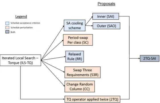
Figure 3.1 shows an overview of all our modifications: modifications pertaining to how a solution is accepted (schedule acceptance criterion) are painted blue, modifications pertaining to how a schedule is perturbed are painted red and the rest is painted purple which is both modifications in one.
3.1 Input Encoding
Requirements are represented as a C × T matrix where C is the number of classes, and T is the number of teachers. Each cell has a three-tuple (θ, γ, µ) that belongs to the requirement that has c as a class, andt as a teacher, θ as the duration in timeslots, γ as times per day, and µas the minimum number of weekly double lessons. Requirements are represented that way since the pair (c, t) for each requirement is unique for each instance.
This is logically represented as a vector of length C × T. Although there are empty cells in this representation, access to each requirement is fast since it is all in a contiguous memory block. Empty cells are represented as (0,0,0).
Teacher unavailabilities are represented as a T × P matrix where T is the total number of teachers and P is the total number of periods. Each cell has a value of 1 or 0 where 1 means the teacher t is unavailable at period p, and 0 means otherwise. This is logically represented as a vector of length T × P. Access to each position (t, p) is fast since all values are in a contiguous memory block.
Figure 3.1: Overview of all our modifications. Blue modifications change how a solu- tion is accepted; red modifications change how a solution is perturbed and the purple modification combines both.
3.2 Constraint Violation Calculation
The calculation of all objective functions was done by using the following data structures:
• Teacher timeslots: aT × P matrix that stores how many times teachertteaches in each periodp. This is used to calculate violations to the third hard constraint: a teacher must teach at most one lesson per period. This is logically represented as a vector.
• Assignments: anR × D matrix whereR is the number of requirements, andD is the number of days. It stores the number of times a requirementris taught in a day.
This is used to calculate violations to the fifth hard constraint: each requirement must have less or equal thanγ assignments per day. This is logically represented as a vector.
• Teacher wd: a T × D matrix that stores which days teacher t teaches in each week. This is used to calculate violations to the third soft constraint: the teachers’
schedules should be concentrated on a minimum number of days. This is logically represented as a vector.
• Double lessons: aRvector that stores the number of double lessons a requirement r has per week. This is used to calculate violations to the first soft constraint: each requirement should have at least µ double lessons a week.
• Unavbls: a T × P matrix that stores the teachert that is unavailable at period p where 1 means that the teacher is unavailable at that period, and 0 means otherwise.
This is used to calculate violations to the fourth hard constraint: teachers must not be assigned periods in which they are unavailable. This is logically represented as a vector.
• Idle tbl: a 2DP vector where DP is a number of periods per day. It stores all combinations of idle times in a day. This is used to calculate violations to the second soft constraint: idle periods in the schedule of teachers should be avoided.
While this data structure is efficient, it does not allow instances with more than 5 days or 5 periods per day to be solved since this vector is hard coded.
3.3 Torque Operator (TQ)
The Torque (TQ) operator builds a conflict graph in which each vertex represents a pair of different requirementsri, rj ∈R for a class, and each edge represents a conflict between this pair, and another pair of requirements from another class when two requirements of a class are swapped. After all connected components are identified, each component represents a chain of one or more swap moves that generates a new neighboring solution that minimizes conflicts.
Figure 3.2 shows how the TQ operator is applied to a schedule, that shows teachers’
ids, to build a conflict graph. Two random timeslots (t9 and t15) are selected. If we swap those timeslots for class c0, there is a teacher clash with c2 (i.e. teacher 14 teaches on timeslot t15 at the same time onc0 and c2). So, they are connected in the conflict graph.
There is no conflict withc2 and the rest of the classes, so it is another separate connected component. In the end, there are two connected components, the blue one is chosen, so all pairs of requirements in that connected component are swapped, and the new schedule is a neighbor of the current schedule.
3.4 Constructive Algorithm
Initial solutions are constructed by the randomized heuristic shown in Algorithm 1 by Saviniec and Constantino (2017) that receives a set of requirements R, and for each requirement e that belongs to R, e’s address is stored in p(e), its class is stored in c0 and the number of lessons for that requirement is stored in numLessons. Finally, p(e) is randomly placed in numLessonsempty timeslots for class c0.
Solutions represented this way satisfy the constraints hc1 (i.e. each requirement must be assigned to exactlyθ times a week), and hc2 (i.e. a class must attend exactly one meeting per period). To sum up, the algorithm iterates through all requirements, and randomly assigns them to empty timeslots according to their class.
Figure 3.2: TQ Move applied to a schedule with teachers’ ids, two random timeslots (t9 and t15) are selected. Conflicts are highlighted in blue and red in the conflict graph. The blue connected component is chosen and its requirements are swapped.
Algorithm 1 Pseudo-code of the constructive algorithm by Saviniec and Constantino (2017)
1: function Construct-Solution(R)
2: Initialize an empty solution Z.
3: for each e∈R do
4: Letp(e) be a pointer to e.
5: c0 =e.c
6: numLessons=e.θ
7: while numLessons >0 do
8: Let Pc0 be the subset of timeslots j ∈P for whichZc0j is empty to class c0.
9: Choose a random timeslot j ∈Pc0
10: Zc0j =p(e)
11: numLessons = numLessons - 1
12: end while
13: end for
14: return Z
15: end function
3.5 Iterated Local Search
The local search as seen in Algorithm 2 by Saviniec and Constantino (2017) receives a solution Z as a parameter, setsP as the set of timeslots in the solution, and CC as the connected components in a graphGof conflicting meetings. The score of the solutionZ is stored inf0, and for every unique timeslot pair (i,j), it constructs the conflict graphGof solution Z and updatesCC to store the connected components ofG. For every connected component k in CC, all the requirements in k are swapped to obtain a new solution Z00 that will replace the current solution Z if it is not worse. The algorithm stops until no further improvement is made compared tof0. To sum it up, it builds a new conflict graph for every period pair, and for every component of the graph, it swaps all nodes that belong to that component, and the new solution is changed to be the best one if it is not worse than the current one. It stops until no more improvement is made.
Algorithm 2 Pseudo-code of the local search with the TQ operator by Saviniec and Constantino (2017)
1: function LocalSearchTQ(Z)
2: Let P be the set of timeslots defined in Section 4.1.
3: Let CC be the set of connected components in a graphG of conflicting meetings.
4: do
5: f0 =f(Z)
6: for each (i, j ∈P;i6=j) do
7: Construct the graph G for requirements assigned to timeslots i, and j of solution Z.
8: Compute the connected components of G, and update CC.
9: for each (k∈CC) do
10: Swap the requirements at the component k to obtain a neighboring solution Z00.
11: if f(Z00)≤f(Z)then
12: Z =Z00
13: end if
14: end for
15: end for
16: while f(Z)< f0
17: return Z
18: end function
The implementation of Algorithm 3 by Saviniec and Constantino (2017) is similar to the classic ILS: it starts with a solution Z and the number of seconds stored in tmax, the best solutionZ∗ is initially the current solutionZ. The solution is perturbed by applying one TQ move, and then it is local searched to improve the solution Z, if this solution is strictly better than the best one found so far, then the counter N otImproved goes back to 0. Otherwise, it is incremented. The best solution is stored inZ∗ if the current solution not worse than the best one. If there was no improvement in the last 3 iterations, the counter is reset and the current solution is the best one. Here, the modification to the classic ILS is given by the number of times the current solution shows no improvement: if it is equal or greater than three, then it resets the current solution to the best one found so far. The implementation runs for tmax seconds.
Algorithm 3 Pseudo-code of the ILS-TQ algorithm by Saviniec and Constantino (2017)
1: function ILS-TQ(Z, tmax)
2: Z∗ =Z.
3: NotImproved = 0.
4: while CpuT ime()< tmax do
5: Z =P erturbation(Z,1)
6: Z =LocalSearchT Q(Z)
7: if f(Z)< f(Z∗) then
8: N otImproved= 0
9: else
10: N otImproved=N otImproved+ 1
11: end if
12: if f(Z)≤f(Z∗) then
13: Z∗ =Z
14: end if
15: if N otImproved≥3 then
16: Z =Z∗
17: N otImproved= 0
18: end if
19: end while
20: return Z∗
21: end function
3.6 Modifications
The perturbation phase of Saviniec et al.’s method consists of a single TQ move that ran- domly chooses between two periods. We believe that a modification in this perturbation phase will help improve its results if it is explored more. Furthermore, applying relaxed rules might help find a better solution.
3.6.1 Two ILS-TQ (2TQ)
The problem with a single random TQ move is that it might get canceled in the local search phase with another TQ move. So, in order for this not to happen, two TQ moves are applied instead of one.
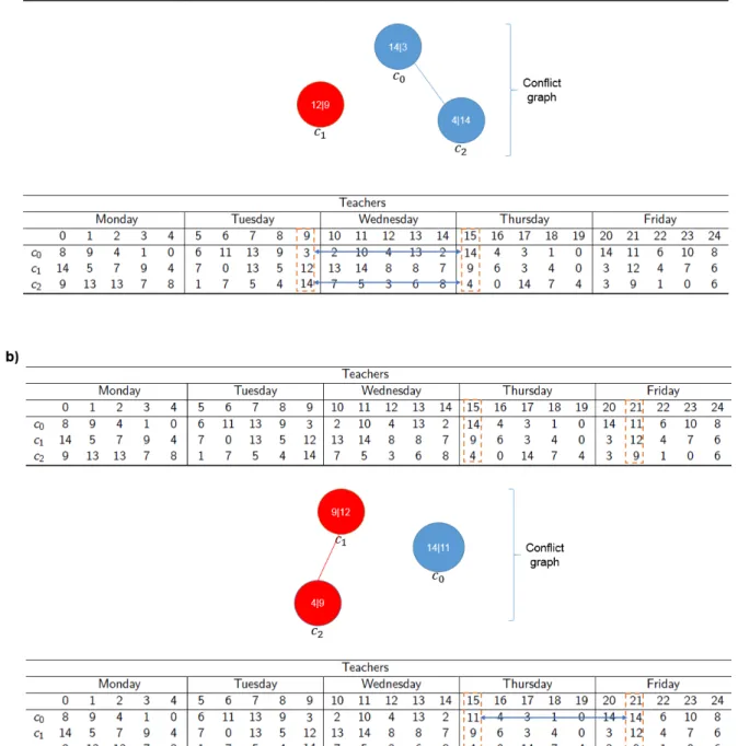
Figure 3.3 shows an example of this method applied to a schedule with teachers’ ids.
The timeslots are randomly selected, the second conflict graph is built after one connected component from the first graph has been swapped. The new schedule after the second TQ move is the new neighbor. The blue component from the first conflict graph has been chosen, and the green component from the second conflict graph was chosen.
Figure 3.3: 2TQ applied to two schedules with teachers’ ids. a) two random timeslots (t9 and t15) are selected and the requirements in the blue connected component are swapped.
b) Two random timeslots (t4 and t10) are selected and the components in the green connected component are swapped. Conflicts are highlighted in blue, red and green in the conflict graphs.
Figure 3.4: RR applied to one schedule with teachers’ ids. The upper schedule S is the best found so far, and the lower schedule S0 is the current one after a local search. Its new score is only to compare against the best solution found.
3.6.2 Relaxed Rule (RR)
The original ILS-TQ has no relaxed rules, meaning that it will not accept solutions that are worse than the best one. This is not a perturbation operator per se, but it will allow more solutions to be explored. This is a rule used by Fonseca and Santos (2014) that im- proved over their variations. In other words, the evaluation function of the new solution f(S”) is replaced by f(S”)−α × ρ(S, S”) where S” is the new solution, S is the best solution, α is 1.0, andρ(S, S”) is the distance between the two solutions (i.e. the number of cells between the two solutions are different). This relaxed rule is placed at Line 11 in Algorithm 2
Figure 3.4 shows this relaxed rule applied to a scheduleS0 that has been found after a local search (i.e. lower schedule). The upper schedule S is the best schedule that has a score of f(S), whereas the current schedule has a score of f(S0), its new score is only used to compare against the best solution found.
3.6.3 Random Swaps per Class (SC)
This perturbation consists in swapping two random periods for each class that is chosen randomly. This perturbation does not get canceled like the original perturbation phase.
This is a modified version of the local search used in the second SA by Zhang et al. (2010).
Figure 3.5 shows an example of this method applied to a schedule with teachers’
ids. Classes are selected in a random order and timeslots are randomly chosen. For c0, timeslots t4 andt16 are swapped;c2, timeslotst3 and t7 are swapped;c1, timeslotst19and t20 are swapped.
Figure 3.5: SC applied to the current schedule with teachers’ ids. In each step, a random new class is chosen, and two timeslots are randomly chosen to be swapped.
3.6.4 Change Random Column (CC)
This move copies a random i−th column of the best solution to the current solution’s i−th column, and replaces the new solution’s requirements with extra periods with those that lack periods. This is one operator used by the technique by Skoullis et al. (2016)
Figure 3.6 shows how this method is applied to the current schedule. The fifth column (i.e. timeslot t4) was randomly chosen from the best schedule (upper one) to be copied to the current schedule. However, in order to copy this column, timeslots t4 and t11 are chosen for class c0, and timeslots t4 and t7 are chosen for class c1 to be swapped so that the current solution’s second column can be the same as the best schedule’s.
3.6.5 Swap Three Requirements (S3R)
This operator swaps requirements r1, and r2, and then it swaps requirements r2, and r3 for each node in the components generated in the two conflict graphs for three random timeslots t1, t2, t3. This is a modification of the operator by Yousef et al. (2013), but applying the TQ operator.
Figure 3.6: CC applied to the current schedule with teachers’ ids with timeslot t4 as the chosen column to copy from the best schedule. Timeslotst11and t7 are chosen for classes c0 andc1 respectively, and swapped with timeslott4. Finally, the column has been copied.
Figure 3.7 shows an example of this method applied to a current schedule. This is similar to the method 2TQ, except for the fact that the last timeslot chosen in the first TQ move is the first timeslot chosen in the second TQ move. In this case, timeslots t9 and t15 have been chosen in this order for the first TQ move, and the blue connected component has been chosen. So, timeslots t15 and t21 have been chosen in this order for the second TQ move, and the blue connected component has also been chosen.
3.6.6 Simulated Annealing (SA) Cooling Scheme
We decided to implement the SA cooling scheme within our implementation of the Iterated Local Search Torque ILS-TQ. Similar to the method RR, this may also accept worse re- sults, but according to the following criterion: r < ef(S)−f(S”)t modified from Zhang et al.
(2010) where r is a random number between 0 and 1 inclusive, f(S) is the score of the best solution, f(S”) is the score of the current solution and t is the temperature. The latter is a parameter that is tuned, but the temperature changes according to a cooling scheme given by t = α×t where α is the cooling rate and this parameter is also tuned.
The criterion is placed in the local search and evaluated when the current solution S” is worse than the best solution found so far S (i.e. after Line 12 in Algorithm 2). However, the cooling scheme can be placed at the end of each iteration or at the end of each loop in the local search (the temperature is reset at the start of each local search). The former is the SAO whereas the latter is the SAI. A hybrid method is also proposed using the SAI
Figure 3.7: S3R applied to one schedule with teachers’ ids. a) TQ move applied to the current schedule. b) Another TQ move applied to the new schedule with timeslot t15 as the common timeslot. Conflicts are highlighted in blue and red in the conflict graphs.
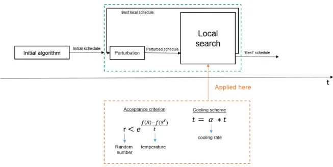
Figure 3.8: SAI overview. Both the acceptance criterion and the cooling scheme are applied inside the local search, the latter is applied at the end of the local search.
cooling scheme and the 2TQ perturbation operator.
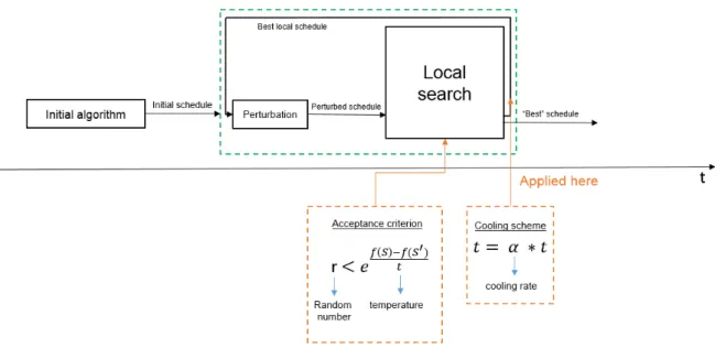
Figure 3.8 and Figure 3.9 show the difference between the SAI and the SAO. The difference is that the former applies the cooling scheme inside the local search (i.e. after Line 15 in Algorithm 2), whereas the latter applies the cooling scheme outside and after the local search (i.e. after Line 18 in Algorithm 3).
3.7 HSTTP Instance Creator
Creating instances following the XML format used for this problem is a tedious task since there are multiples requirements per class and teacher unavailabilities. On this creator as seen in Figure 3.10, users can enter the number of classes, teachers, days, and periods for the schedule. After that, the ”Generate” button generates two matrices of size T ×3 and T ×D×P respectively where T is the number of teachers, D is the number of days, and P is the number of periods per day. In the first matrix, users can create requirements by choosing a class in the combobox, the teacher row, and entering the Lessons (i.e. total number of lessons), M ax (i.e. maximum number lessons per day), DLessons (i.e. min- imum number of double lessons). Requirements that have 0 lessons are ignored. In the second matrix, the user can define teachers’ unavailabilities by clicking on any button that corresponds to the teacher, the day (i.e. the number in each button) and the period (the number above each button); if the button is green, it means that the teacher is available on that period, if it is red, it means that the teacher is unavailable on that period. Then, the user can click on the ”Finish” button to generate the XML file. This form was created in C# on Visual Studio Community 2015.
Figure 3.9: SAO overview. Only the acceptance criterion is inside the local search, but the cooling scheme is applied outside the local search at the end of the iteration of the meta-heuristic.
Figure 3.10: HSTTP instance creator user interface
Figure 3.11: HSTTP instance creator XML output
Figure 3.11 shows the XML output of the creator given the input parameters shown in Figure 3.10, class 0 also has requirements that cannot be seen in the latter figure.
Although this instance is not valid, it is still shown to give an idea about what this creator generates.
3.8 Final Considerations
The method proposed by Saviniec and Constantino (2017) does not mention how the constraint violations are calculated or what data structures they used to calculate them, so we mentioned what data structures we used. Our modifications are done to the per- turbation phase, the original method uses one random TQ move, but the main problem with it is that it might get canceled in the local search. So, we are going to implement the following: two TQ moves, Relaxed rule, Random swaps per class, Change random column, and Swap Three Requirements. In the following section, the results to these changes are compared to the original method. Furthermore, the HSTTP instanc