Furthermore, the fulfillment of the involution in the weak sense when the mesh parameter goes to zero is shown. Some numerical examples illustrate the behavior of nonlocal solutions to the problem, in particular the clustering phenomenon.
Introduction
- Scope
- Assumptions
- Motivation
- Related work
- Outline of the chapter
In the highly degenerate case, solutions of the nonlocal problem are usually discontinuous and must be defined as weak solutions. The interpretation of (1.1) as a model for the aggregation of populations (e.g. of animals) can be illustrated as follows.
Definition of a weak solution
It is easy to check that the entropy solution to the initial value problem is a weak solution. The following lemma states that, conversely, every weak solution to the initial value problem is an entropy solution.
Jump conditions and uniqueness
Rankine-Hugoniot condition
Uniqueness of weak solutions
Convergence analysis of numerical schemes
- Preliminaries
- Uniform estimates on {v n j } and {u n j+1/2 }
- Convergence to the weak solution
- Finite Speed of Propagation
In Lemma 1.4.1 we prove that the v-scheme is monotonic, and derive from this that the numerical solution {vnj} satisfies an L1Lipschitz continuity in time property (Lemma 1.4.2). Then we prove in Lemma 1.4.4 that the spatial total variation of A(Un) is uniformly bounded. 2 Lemma 1.4.4 generally does not allow establishing a uniform bound on the spatial total variation TV(Un) of the solution values{unj+1/2}generated by the u scheme.
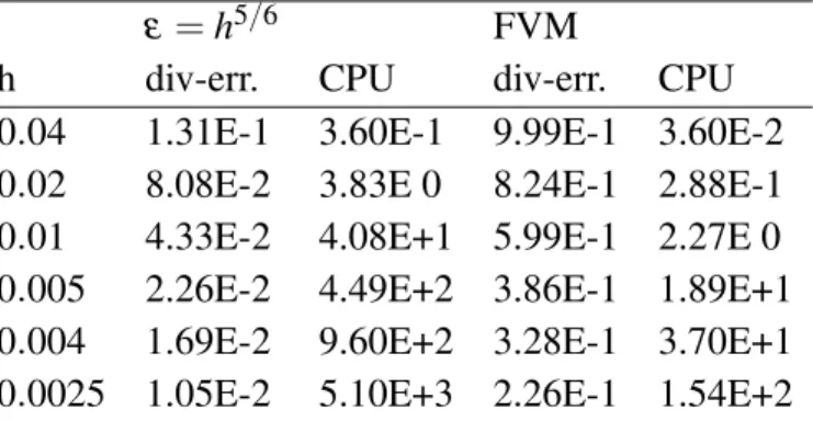
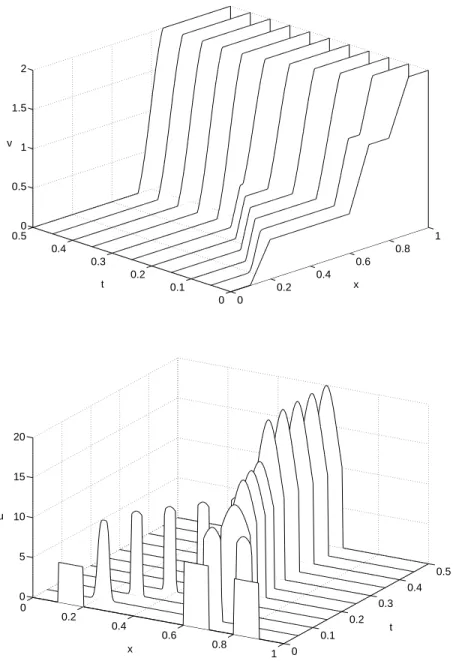
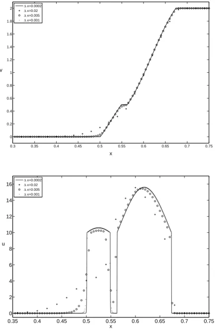
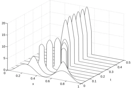
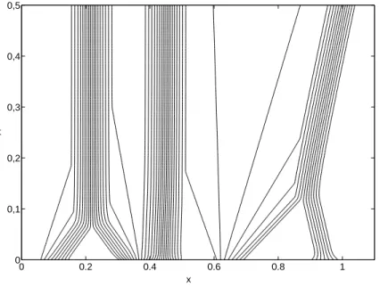
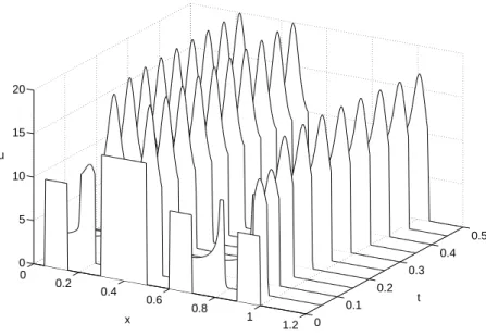
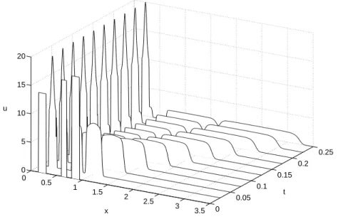
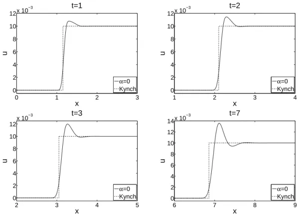
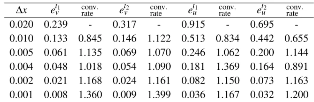
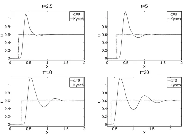
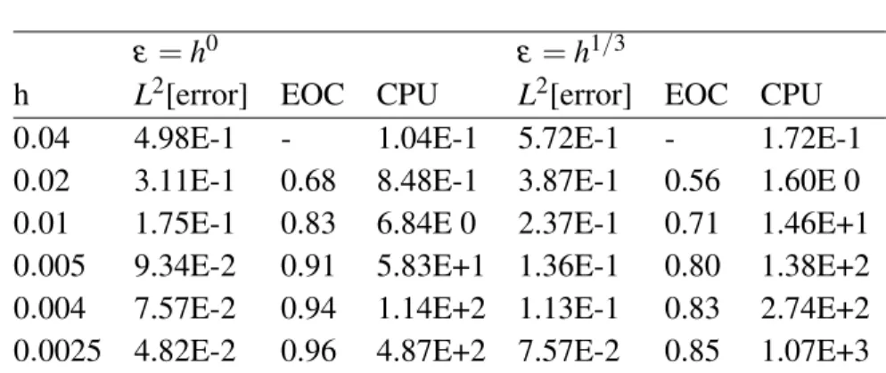
Let us assume that v∗ In addition to Figure 1.5, we show in Figure 1.6 a contour plot of the numerical approximation of v for this example. Clearly, (2.1) can be considered as a non-local version of the kinematic sedimentation model due to Kynch [70] which gives rise to the local scalar conservation law. It seems to us that only (2.9) is suitable for simulating the complete sedimentation process from the dilute boundary to the densely packed bed. But for α ≥1 the expression inside the derivative on the right-hand side of (2.10) is multiplied by du(1−u), regardless of the algebraic form of V, so for u=0 and u=1 (2.10) degenerates to. We state some assumptions about the functions su0andV and about the mask of the numerical scheme and derive some estimates of differences in the discrete convolution. Conclusions, limitations and possible extensions are addressed in section 2.7. of all particles and the nature of boundaries, if any [52]. Equation (2.16) does not contradict the result that the velocity of the test sphere is affected by all the spheres in a suspension, because the velocity variance is determined by the positions of all the spheres [108]. Although the velocity of the spheres relative to the liquid is independent of the shape of the container [13], equation (2.17) applies only to dilute suspensions that settle towards an infinite flat plate. The Richardson-Zaki equation [100] (2.6), corresponding to V(u) given by (2.3), is widely used to predict the interface position and the propagation of concentration changes. In the Pickard-Tory model, the dependence of the settling velocity, vs(x0,t), onc(x0,t) instead of u(x0,t) is similar to the dependence in [11], but not as specific. Layered sedimentation in suspensions The obvious difficulty in defining a numerical scheme for (2.1) arises from the discretization of the integral. The calculations and numerical analysis are based on the Lax-Friedrichs scheme for a standard non-linear scalar conservation law. We summarize all assumptions about the initial datumu0, the velocity function V and the grid. Applying the last two inequalities to the right-hand side of (2.23) and using thatu∆(·,tn)∈L1loc(R), we obtain. In what follows, Ca always denotes a constant that is independent of ∆:= (∆x,∆t) but depends on one and which can change from one line to the next. Moreover, the discontinuity between two values of the solution must satisfy the following jump entropy condition, which is a consequence of (2.27): By inserting the last terms into the integrands in (2.30) using the properties of the Ka kernel and the fact that it has bounded variation we arrive at . Due to the CFL condition, the last right-hand side is a convex combination of unj+1, unj−1 and one. Using Lemma 2.3.2, we can prove the following unitary limit of the total variation of the numerical approximation generated by (2.31). Summing over j and using Lemma 2.5.1, we find that there are constants C6 and C7 that depend on but not on ∆, so that. Then, using the u∆ is Lipschitz continuous respecting the space variable and Lemma 2.3.1, we get that the solution generated by the numerical method converges to a Lipschitz continuous function. The "viscous shock" type solution is of particular interest in the context of the sedimentation model, as it corresponds to the evolution of the suspension-supernate interface.). As predicted in Section 2.2.2, we obtain the formation of low mass due to the non-constancy of the initial data. We assume a stronger oscillatory behavior where meta=0.2 and ena=0.1, and that the period of the oscillation is proportional to the value of for both cases. The obvious problem occurs when we are "close" to the boundary, since in a batch process we have a zero flux condition and for the numerical calculations we have to extrapolate values to calculate the numerical fluxes. We also use a non-linear color scale to emphasize the layering phenomenon, which is supposed to appear in the concentration range close to the original concentration. We also see, if we compare Figures 2.10 and 2.12, that the "width" of the layer is proportional to the parametera. Unfortunately, most of the constants that appear in the compactness estimates in Section 2.5.1 are not uniform with respect to a, i.e. it is proved for Finite-Volume schemes that the discrete solution of the extended system converges to the weak solution of the original system for vanishing discretization and expansion parameter under appropriate scalings. The proofs rely on a reformulation of the expansion as a relaxation-type approximation and careful use of the convergence theory for Finite-Volume methods for systems of Friedrich's type. The solutions of the equations of linear elasticity must satisfy compatibility conditions on the strain gradient, which results in an involution condition (cf. Chapter 5 in [39]). Another example is a linear piezoelectric system (see [84]). By carefully investigating the convergence theory of Vila and Villedieu [112] and Jovanovic and Rohde [59], we obtain (see Theorem. The key fact is that the estimate does not depend critically on the parametersε. In particular, it is clear that we are again within the framework of symmetric systems, and the extended formulation leads to a hyperbolic system. We want a generic estimate (as in Theorem 3.2.1) for the system (3.9), but it is not clear how the constant will depend on ε. To obtain estimates for kuεtk andkϕtεk we use (3.9), the limit for kUεk2. Proposition 3.2.1 shows the equivalence of the solutions of the extended formulation (3.9) and the solution of the original problem for ε>0. However, it is not clear how ε can be solved (asymptotically) in the calculation and whether the constraint (3.3) is satisfied in the limit. Aε,ne,K =OTΛ+O+OTΛ−O, (3.13) where Λ+(Λ−) is a diagonal matrix whose entries are positive (negative) eigenvalues of Aε,ne,K. However, we will choose ε =ε(h)withε(h)→0 as h→0, so that the GLM-FV method should satisfy the constraint (3.3) whenever the classical FVM does not. The key question here is how to determine ε(h) to obtain the (optimal order of) convergence and satisfy the side condition (3.3). With Lemma 3.4.1 we can now prove a global L2 stability result as discrete counterpart to Lemma 3.2.1. A Comparison Result We conclude with the proof of Theorem 3.4.1. Using Proposition 3.4.2 and Lemma 3.4.2 with ω =θ and π=θUε we only need to estimate. Returning to the first term of R.H.S in (3.35), we notice that thanks to Green's formula we find ∑e∈∂K∑di=1nie,K(Aε,i)nKUKε(t)θ(t)|e|=0 .Therefore using the last expression and Green's formula we have that For example, using the Cauchy-Schwarz inequality, Lemma 3.4.3, the regularity of F and θ, Theorem 3.2.2, and the CFL condition, we obtain Numerical results will show the role of ε in maintaining the constraint at the numerical level. In Example 3.5.3 we will see that the absence of ε results in serious problems in involution. This parameter can potentially improve the convergence speed of the involution, at least in the weak sense. Initial condition for E1, E2 and B3 are chosen according to (3.42) together with the results for the application of the GLM-FV method. This is not a surprise, because the predicted rate in the case without including the involution (FVM) is 1/2 [112]. We do not show the error in the discrete calculation of ∇·E because ∇·E=0 is preserved in machine precision. Example 3.5.1 suggests that using the GLM-FV method does not pay off as the higher computational cost comes with an even worse convergence rate (compared to the original FV method). The following three examples show the advantages of the approach when the divergence error becomes more important. The idea behind this numerical example is to study the behavior of the discrete version of ∇·B generated by the GLM-FV approximation. We see that for both methods (FV and GLM-FV) the error in ∇·B converges to zero. However, we also notice that the error of the GLM-FV method remains much lower than that of the FV method and, in addition, we obtain better results for smaller values of ε =ε(h). We now want to study the behavior of the GLM-FV method for the Maxwell equations under a small perturbation in the condition∇·j=0. This approach is a generalization of the approach for the equations of electrodynamics due to. Numerical examples illustrated the performance of the method on the Maxwell equations and the induction equation in MHD. Convergence of locally divergence-free discontinuous Galerkin methods to the induction equations for the 2D-MHD equations. Asymptotic behavior of interfaces to a nonlinear degenerate diffusion equation in population dynamics. Japan J.Numerical examples
Motivation of the nonlocal sedimentation model
Nonlocal dependence of settling velocities
Preliminaries
Assumptions and numerical scheme
Definition and uniquenss of entropy solutions
Definition of an entropy solution and jump conditions
Uniqueness of entropy solutions
Convergence analysis and existence of entropy solutions
Numerical Examples
Conclusions
Preliminaries
Finite-Volume Discretization
Convergence of the GLM-FV scheme
Stability results
The Error Estimate
Numerical Examples
Example 1
Example 2
Example 3