Hyperbolic structures on surfaces and geodesic currents
Javier Aramayona and Christopher J. Leininger January 31, 2014
Abstract
These are lecture notes for a course given by the authors during the program Automorphisms of Free Groups: Geometry, Topology, and Dynamics, held at the CRM (Barcelona) in 2012. The main objec- tive of the notes is to describe Bonahon’s construction of Thurston’s compactification of Teichm¨uller space, in terms of geodesic currents on surfaces. In the final section, we present several extensions of the notion of geodesic current to various other more general settings.
1 Introduction
This chapter contains the lecture notes from the course “Hyperbolic struc- tures on surfaces and geodesic currents”, given by the authors during the summer school onAutomorphisms of Free Groups: Geometry, Topology, and Dynamics, held at the CRM (Barcelona) in September 2012. The main ob- jective of the notes is to give an account of Bonahon’s description [5] of Thurston’s compactification of Teichm¨uller space in terms of geodesic cur- rents on surfaces. The plan of the chapter is as follows. Section 2 deals with hyperbolic structures on surfaces, explaining why a surface equipped with a complete hyperbolic structure is isometric to the quotient ofH2 by a Fuch- sian group. In Section 3 we will review some basic features of Teichm¨uller spaces and measured geodesic laminations, ending with some words about the “classical” construction of Thurston’s compactification. In Section 4, we will introduce geodesic currents, and explain Bonahon’s interpretation of the compactification of Teichm¨uller space. Finally, in Section 5 we will present some generalizations of the notion of geodesic currents to other set- tings, such as negatively curved metrics on surfaces, flat metrics on surfaces, and free groups.
The main references for the material presented here are [1,4,5,14,15,29].
Acknowledgements. We would like to thank Juan Souto for conversations.
The second author was partially supported by NSF grant DMS-1207183.
2 Hyperbolic structures on surfaces
In this section, we briefly discuss the notion of ahyperbolic structure on an oriented topological surfaceS, and explain why a surface equipped with a complete hyperbolic surface is isometric to the quotient of the hyperbolic plane H2 by a discrete subgroup of PSL(2,R), the group of orientation- preserving isometries of H2. We refer the reader to the sources [2, 3, 10, 11, 24, 33] for more detailed accounts of the topics treated here.
Definition 2.1 (Hyperbolic structure). Let S be an oriented topological surface without boundary. A hyperbolic structure onS consists of an open cover (Ui)i∈I of S, together with maps ψi :Ui →H2, such that
1. ψi is an orientation-preserving homeomorphism onto its image, for all i∈I, and
2. Whenever Ui∩Uj 6= ∅, the restriction of ψj ◦ψ−1i to each connected component ofψi(Ui∩Uj) is an orientation-preserving isometry ofH2, that is, an element of PSL(2,R).
A surface equipped with a hyperbolic structure will be called a hyperbolic surface.
Each pair (Ui, ψi) is called achart. Observe that a hyperbolic structure determines a Riemannian metric on S by declaring each map ψi in the definition above to be an isometry (in particular, this endows S with a smooth structure). In this way we can talk about the length of a (rectifiable) path on S; we say that a path on S is a geodesic if it locally minimizes distance between its points.
We next present two constructions of hyperbolic surfaces.
Example 1. Let Γ be a torsion free Fuchsian group, that is, a subgroup of PSL(2,R) acting freely and properly discontinuously onH2. ThenS=H2/Γ is a surface andp:H2→S is a covering map. Let (Ui)i∈I be a collection of evenly covered open sets ofS whose union coversS, and letψi :Ui→H2 be a continuous 1–sided inverse to p (which exists since Ui is evenly covered).
In this way, we see that the open sets (Ui), together with the maps ψi, give an example of a hyperbolic structureS =H2/Γ.
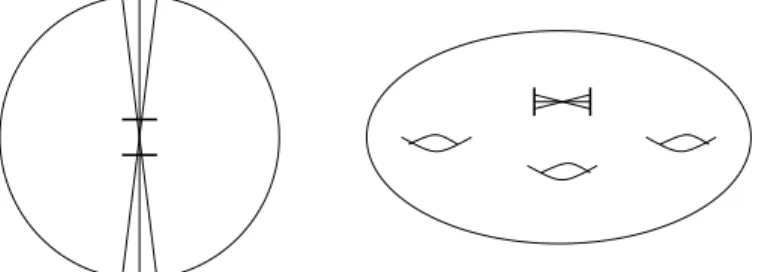
Example 2. Let P be a regular hyperbolic 4g–gon with internal angle π/2g, where g ≥2 is an integer. Let S be the closed orientable surface of genusgobtained by gluing the opposite sides ofP by hyperbolic isometries;
see Figure 1. The surface S admits a hyperbolic structure determined by charts defined on open subsets obtained from disks in the interior of P, or constructed by gluing half-disks or sectors of disks about points in the boundary of P; see again Figure 1. In fact, Poincar´e’s Polygon Theorem (see, for instance, [24]) tells us that this example is essentially equivalent to the one above; for instance, the Fuchsian group Γ of Example 1 is generated by the hyperbolic isometries used to identify the sides of the polygon.
d
d c
c b
b
a
a
Figure 1: A regular hyperbolic octagon with internal angle π/4. Gluing opposite edges of the polygon renders a closed surface of genus 2, which is naturally equipped with a hyperbolic structure: the diagram shows charts around a point, depending on whether a lift of the point lies in the interior, on a side, or at a vertex of the polygon.
The following theorem states that Example 1 is the unique source ofcom- plete hyperbolic structures, that is, those hyperbolic structures that make the surface into a complete metric space; we refer the reader to [8] for a nice discussion of incomplete hyperbolic structures.
Theorem 2.2 (Cartan-Hadamard). Suppose S is equipped with a complete hyperbolic structure. Then S is isometrically diffeomorphic to H2/Γ, where Γ is a torsion free Fuchsian group.
In particular, if S is a closed surface equipped with a hyperbolic struc-
ture, then S is (isometrically diffeomorphic to) the quotient of H2 by a Fuchsian group.
The idea of the proof of Theorem 2.2 is as follows; see [3] for a detailed proof. Suppose thatS is equipped with a hyperbolic structure, with charts (Ui, ψi)i∈I. Choose x ∈ S and, up to relabeling, assume we have a chart defined on an open set U1 containing x. Given a path α: [0,1] → S with γ(0) = x, we cover it with domains of charts U1, . . . , Un such that only consecutive sets intersect and such that there is a subdivision 0 = t0 <
t1 < . . . < tn = 1 with α([ti−1, ti])⊂Ui for each i= 1, . . . , n; furthermore, up to refining the cover, we may assume that the intersection of any two consecutive open sets is connected. Using the fact that ψi and ψi+1 differ by an element gi ∈PSL(2,R)
ψi =gi◦ψi+1
we may construct a pathαH: [0,1]→H2 starting at ψ1(x) so that for each i, αH|[ti−1,ti] agrees with ψi◦γ|[ti−1,ti], up to composing with an element of PSL(2,R); one can check that the terminal endpoint ofαH only depends on the homotopy class ofα, rel endpoints. In this way we obtain a map
Dev : ˜S →H2,
where ˜S denotes the universal cover of S, which associates to each α ∈S,˜ the endpoint of αH. By construction, the map Dev, called the developing map, is a locally isometric diffeomorphism onto its image, where ˜S has been equipped with the unique Riemannian metric that turns the natural covering map ˜S →S into a Riemannian covering map.
In a similar fashion, to each α∈π1(S, x) we associate a unique element of PSL(2,R), namely the composition g1◦. . .◦gn−1 of the maps associated to the consecutive pairs of the setsU1, . . . , Un chosen to cover α, where we assume U1 =Un. As above, the element of PSL(2,R) depends only on the homotopy class ofα rel basepoint, and thus we obtain a map
Hol :π1(S, x)→PSL(2,R), called theholonomy homomorphism.
One can check that with the action of π1(S) on ˜S, Dev is equivariant with respect to Hol:
Dev(α·z) = Hol(α)·Dev(z).
The completeness assumption shows that Dev is a covering map. Since ˜S andH2 are simply connected, it is a homeomorphism and hence an isomet- ric diffeomorphism. At this point, it follows from standard covering space
theory that Hol is an injective homomorphism and the image is a Fuchsian group.
Remark 1. The construction of the maps Dev and Hol depend on the choice of basepoint and initial chart. However, the developing maps corre- sponding to two different choices differ by an isometry and the holonomy homomorphisms differ by conjugation in PSL(2,R). See [3] for details.
3 Teichm¨ uller space
Throughout the remainder of these notes,S will be assumed to be a closed oriented surface of genusg≥2. This is for simplicity in this section, but in later sections this assumption is necessary not just for the proofs, but for the results themselves.
Theorem 2.2 yields that S admits a complete hyperbolic structure. In this section, we introduce the Teichm¨uller space of all hyperbolic structures on S, up to equivalence, and explain why it is homeomorphic to an open subset ofR6g−6. We will end the section by briefly introducing Thurston’s compactification of Teichm¨uller space in terms of measured geodesic lami- nationson S.
A convenient way to think of a hyperbolic structure onS is as a marked hyperbolic surface.
Definition 3.1. A marked hyperbolic surface is a pair (X, f) where 1. X=H2/Γ is a hyperbolic surface, and
2. f:S →X is an orientation-preserving homeomorphism.
Given a marked hyperbolic surface (X, f), we can pull back the hyper- bolic structure on X by f to one on S. Conversely, given a hyperbolic structure onS, the identity mapid:S →S makes (S, id) into a marked hy- perbolic surface. That said, the notion of marked hyperbolic surface is more convenient for many purposes. Now we give the definition of Teichm¨uller space, as a set.
Definition 3.2. The Teichm¨uller spaceof S is the set T(S) ={(X, f)}/∼
of equivalence classes of marked hyperbolic surfaces, where two marked hy- perbolic surfaces(X, f) and(Y, h)are deemed equivalent if h◦f−1 is homo- topic to an isometryX →Y.
In order to relax notation, we will denote a point [(X, f)] ∈ T(S) by (X, f), or simply by X with the marking homeomorphism implicit.
This definition of Teichm¨uller space gives a natural way to endow it with a topology. Given [(X, f)] ∈ T(S), we can choose an isomorphism π1(X) = Γ<PSL(2,R), and then we have
f∗:π1(S)→π1(X) = Γ.
Note that this is just a holonomy homomorphism for the associated hy- perbolic structure on S obtained by pulling back via f. An equivalent marked surface (Y, h) ∼ (X, f) gives rise to a conjugate homomorphism h∗:π1(S)→PSL(2,R), and thus we obtain a map
T(S)→Hom(π1(S),PSL(2,R))/conjugation.
In fact this map is an injection. The set Hom(π1(S),PSL(2,R)) can be given the compact-open topology, where PSL(2,R) is given its natural topology as a quotient of the matrix group SL(2,R) and π1(S) is given the discrete topology. Equivalently, choosing 2g generators for π1(S), we obtain an in- jection
Hom(π1(S),PSL(2,R))→PSL(2,R)2g
where a homomorphism ρ is sent to the 2g–tuple of ρ–images of the gen- erators. The quotient Hom(π1(S),PSL(2,R))/conjugation is then given the quotient topology, and soT(S) is topologized as a subset of this space via the injection above.
The mapping class groupMod(S) ofS is the group of isotopy classes of orientation-preserving homeomorphisms ofS; in other words,
Mod(S) = Homeo+(S)/Homeo0(S),
where Homeo0(S) denotes the connected component of the identity map in the orientation-preserving homeomorphism group Homeo+(S). The map- ping class group acts naturally on T(S) by changing the marking; namely, givenφ∈Mod(S) and X= [(X, f)], we define
φ(X) = [(X, f ◦φˆ−1)],
where ˆφ denotes a representative of φ. This action is discrete and prop- erly discontinuous (see [15], for instance); the quotient T(S)/Mod(S) is the classical moduli spaceof S.
3.1 Length functions
As we shall see,T(S) is not compact. Thurston [33] constructed a Mod(S)- invariant compactification of T(S) in terms of measured laminations on S, which may be regarded as limits of simple closed curves on the surface; com- pare with the paragraph preceding Theorem 3.6 below. Thurston’s strategy to construct the compactification is to use length functions to embed T(S) into the function spaceRS(S), whereS(S) denotes the set of all isotopy classes of simple closed curves on S, and then understand the closure of T(S) in the projectivized spacePRS(S); this is explained in detail in [1], for instance.
Although this is not the approach that we will follow here, we give a brief account of this construction; along the way, we will obtain a more concrete, geometric description of Teichm¨uller space and its topology. We refer the reader to [1] for a complete discussion of the material discussed here.
Let (X, f) be a marked hyperbolic surface, where X = H2/Γ and Γ is a Fuchsian group. Given an (isotopy class of) simple closed curveα on S, there is a unique simple closed geodesic on X homotopic to f(α). This is the projection of the axis of the element f∗(α) ∈ Γ, where we have chosen a basepoint onα and an isomorphismπ1(X) = Γ. Equivalently,f∗(α) is a hyperbolic isometry fixing the (ideal) endpoints of a lift of f(α). We note thatf∗(α) is only well-defined up to conjugacy in Γ depending on the choices involved, but the resulting geodesic inX is independent of these choices.
For every simple closed curve α ⊂ S and marked hyperbolic surface (X, f), we define
`α([(X, f)]) = length(f(α))
where length(f(α)) denotes the length, measured in the hyperbolic metric onX, of the unique simple closed geodesic homotopic tof(α). An equivalent marked hyperbolic surface (Y, h)∼(X, f) gives the same value, so for every simple closed curveα⊂S there is a well-defined function
`α:T(S)→R.
To relax notation, we often write`α(X) for `α([(X, f)]), with the marking implicit.
There is an explicit relation between `α(X) and the trace tr(f∗(α)) of f∗(α), viewed as an element of Γ (up to conjugacy); namely
tr2(f∗(α)) = 4 cosh2
`α(X) 2
(1) (see, for instance, [3]). As a consequence, length functions are continuous functions on Teichm¨uller space.
Consider the map
L:T(S)→RS≥0(S)
defined asL(X) = (`α(X))α∈S(S). GivingRS≥0(S) the product topology, turns L into a continuous map. Observe that there is a natural action of R+ on RS≥0(S)\ {0}. Denoting the quotient space of this action byPRS≥0(S), we have the following result [1]:
Theorem 3.3. The map
L:T(S)→RS≥0(S)
is a proper embedding. Furthermore the composition of L with the quotient map RS≥0(S)\ {0} →PRS≥0(S) gives an embedding T(S)→PRS≥0(S).
Our next goal is to give an idea of the proof of Theorem 3.3. Along the way we introduceFenchel-Nielsen coordinates, which serve to give a concrete description ofT(S) as an open subset ofR6g−6.
3.2 Fenchel-Nielsen coordinates
It is a standard fact in plane hyperbolic geometry (see, for instance, Propo- sition 10.4 of [15]) that, for any a, b, c > 0, there is a right-angled hyper- bolic hexagon with three non-consecutive sides of lengtha, b, c, respectively;
moreover, such a hexagon is unique up to an isometry of H2. As a conse- quence, any triple (a, b, c) ∈ R3+ determines a unique hyperbolic structure with geodesic boundary1 on a sphere with three boundary components, or pair of pants, in such a way that the boundary components have prescribed lengthsa, b, c.
A pants decomposition of S is a set of (isotopy classes of) simple closed curvesα1, . . . , α3g−3such that every connected component ofS\∪αiis home- omorphic to the interior of a pair of pants. Now, fix a pants decomposition α1, . . . , α3g−3 of S and let X ∈ T(S). If αi, αj, αk bound a pair of pants in S, then by the discussion above, the hyperbolic structure on the sub- surface ofX bounded by the geodesic representatives of f(αi), f(αj), f(αk) is uniquely determined by`αi(X), `αj(X), `αk(X). However, the hyperbolic structure on X is not uniquely determined by these numbers: we need an- other 3g−3 real numbers t1(X), . . . , t3g−3(X), called the twist parameters
1The definition of hyperbolic structure with geodesic boundary is analogous to Defini- tion 2.1, with the modification that the elements of the cover are open subsets of a closed half-space ofH2.
ofX that measure “how twisted” onX the different pairs of pants are with respect to one another; see, for instance, Section 10.6 of [15] for details. The tuple
(`α1(X), . . . , `α3g−3(X), t1(X), . . . , t3g−3(X))
is called theFenchel-Nielsen coordinates of the point X ∈T(S). One then has:
Theorem 3.4. The map
F:T(S)→R3g−3+ ×R3g−3, given by
F(X) = `α1(X), . . . , `α3g−3(X), t1(X), . . . , t3g−3(X) , is a homeomorphism.
The proof of Theorem 3.4 follows quickly from the construction of the coordinates. Indeed, F is continuous since the first 3g−3 are length func- tions, and the last 3g−3 coordinates have simple expressions in terms of the associated homomorphism to PSL(2,R) showing that these are also con- tinuous. Moreover, it is a bijection, as it admits an “obvious” inverse map:
one first starts with a collection of pairs of pants whose boundary compo- nents have length prescribed by the first 3g−3 parameters, and then glues them appropriately according to the twist parameters; again, see Section 10.6 of [15] for details.
Armed with Theorem 3.4, one can show the following stronger version of the first statement of Theorem 3.3:
Theorem 3.5. There exist 9g−9 simple closed curves γ1, . . . , γ9g−9 on S such that the map
N:T(S)→R9g−9≥0 ,
defined as N(X) = (`γi(X))9g−9i=1 , is a proper embedding.
The collection of curves of Theorem 3.5 may be chosen as follows. First, consider a pants decomposition α1, . . . , α3g−3, together with 3g−3 trans- verse curves β1, . . . , β3g−3: these are curves with i(αj, βk) = 0 if j 6= k and i(αj, βj) = 1 or 2, depending on the topological type of the subsurface filled byαj and βj. In addition consider, for each j, the curve β0j obtained by performing a positive Dehn twist to βj along αj; see [15]. The curves {αj, βj, β0j}3g−3j=1 so constructed form the collection of 9g−9 curves whose
existence is claimed by Theorem 3.5. Again,Nis continuous since it is given by length functions. The fact that it is injective follows from a result of Ker- ckhoff [25], which states that the length functions ofβj and βj0 are strictly convex functions of the jth twist parameter tj; see Section 10.6 of [15] for details. Finally, N is proper since the map F of Theorem 3.4 is a homeo- morphism and the lengths of βj, βj0 tend to infinity with tj, whenever the length ofαj is bounded.
Proof of Theorem 3.3. As mentioned above, the first statement is a direct consequence of Theorem 3.5. To see the injectivity of the map T(S) → PRS(S), one proceeds as follows. Let [(X, f)] ∈ T(S), and choose simple closed curvesα, β ⊂S which transversely intersect once. WriteX =H2/Γ, where Γ is a Fuchsian group, and denote byAandBthe realization off∗(α) andf∗(β), respectively, as elements of Γ<PSL(2,R). Now, let γ and δ be, respectively, the positive and negative Dehn twists of α along β. Then γ and δ are realized by the matrices AB and AB−1, respectively. From the trace relation
tr(A) + tr(B) = tr(AB) + tr(AB−1)
in PSL(2,R), plus the relation (1) between trace and length, we obtain a relation between the lengths of α, β, γ, δ which is not invariant by scaling for all choices ofα, β, γ, δ. See [1] for details.
3.3 Measured laminations and Thurston’s compactification of T(S)
We now recall some basic facts about measured geodesic laminations on surfaces, referring the reader to [7, 11, 31] for a detailed account.
We continue to assume S is a closed oriented surface of genus g ≥ 2, which we endow with a fixed hyperbolic structure defining a metric σ. A complete, simpleσ–geodesic on S is an injectively immersed geodesic with respect toσisometric toRor a circle of some length. A(geodesic) lamination onS is a closed subsetL⊂S which may be decomposed as a disjoint union of pairwise disjoint, complete, simpleσ-geodesics on S. The decomposition into simple geodesics depends only on the subset, so the subsetLdetermines the structure as a geodesic lamination. Each geodesic in the decomposition is called aleaf of the lamination.
A transverse measure λon a lamination Lis an assignment of a Radon measureλ|k to each arckon S transverse to L, in a way that:
1. Ifk0 is a subarc of an arck, then λ|k0 is the restriction tok0 ofλ|k;
2. If k, k0 are arcs that are homotopic via a homotopy Ft, such that F1:k→k0 is a homeomorphism and Ft(k) is transverse to the leaves ofLfor all t, thenλ|k0 = (F1)∗(λ|k).
As a consequence of (2), it follows that for any arc k, the support of the measure is contained in the intersectionk∩L. A measured laminationis a pair (L, λ) of a geodesic lamination together with a transverse measure. We often abuse notation and simply writeλinstead of (L, λ).
We denote by ML(S) the set of measured geodesic laminations on S.
Topologize ML(S) by declaring that a sequence (λn)n∈N of measured lami- nations converges to another measured laminationλif
Z
k
f dλn→ Z
k
f dλ;
for every continuous functionf :k→Rwith compact support defined on a generic transverse geodesic arc k⊂S (that is, a geodesic arc transverse to all simple complete geodesics, or equivalently, not contained in any simple complete geodesic).
Remark 2. Observe that the notation ML(S) does not make reference to the fixed hyperbolic metric σ on S that we used to define measured geodesic laminations. The reason for using such notation is that, as we shall see in Section 4 below, for any two choices of hyperbolic metric there is a canonical homeomorphism between the corresponding spaces of measured geodesic laminations.
A first example of a measured geodesic lamination on S is a simple closed geodesic α⊂S, where the transverse measure assigns, to each arc k transverse toα, the Dirac measureµα|k that counts the intersection withα:
µα|k(E) =|E∩α|,
for any Borel subset E ⊂k. More generally, we can consider the weighted measure tµα, where t is a positive real number. Since every isotopy class of simple closed curves has a unique geodesic representative, we thus obtain an injective map
S(S)×R+→ML(S),
given by (α, t)7→tµα. As it turns out, the image of the above map is dense in ML(S) (see, for instance, Theorem 3.1.3 of [31]). There is a slightly weaker result whose proof is less involved, which we explain next. Ifα1, . . . , αn are pairwise disjoint simple closed curves and t1, . . . , tn ∈ R+, then P
itiµαi also defines a measured geodesic lamination called aweighted multicurve.
Theorem 3.6. The subset of ML(S) consisting of weighted multicurves is dense in ML(S).
This theorem follows from the construction of the so-calledDehn-Thurston coordinates for ML(S) (see, for instance, [31]), which may be regarded as an analog for laminations of Fenchel-Nielsen coordinates for Teichm¨uller space. Before describing these coordinates we need some definitions. Given α∈S(S) and λ∈ML(S), the intersection number ofα and λis defined by
i(α, λ) = Z
α∗
dλ
where the integral is over the geodesic representativeα∗ ofα. This general- izes the notion ofgeometric intersection numberi(α, β) between two simple closed curvesαandβ, which is defined as the minimal number of transverse intersection points between representatives of α and β. Indeed, with the notation above,
i(α, β) =i(α, µβ).
More generally, there is a continuous, symmetric, bilinear form i:ML(S)×ML(S)→R,
called the intersection numberform, which extends the usual geometric in- tersection number for pairs (α, β) ∈ S(S)×S(S). In the next section we will give an explicit definition for (a generalization of)iin terms of geodesic currents.
Given a fixed pants decomposition α1, . . . , α3g−3, the associated Dehn- Thurston coordinates forML(S) is a homeomorphism
ML(S)→(R3g−3≥0 ×R3g−3\ {0})/∼ (2) where the first 3g−3 coordinates ofλ∈ML(S) are the intersection numbers i(αi, λ) and the last 3g−3 coordinates{twi(λ)}3g−3i=1 provide a measurement of the twisting ofλaround the curvesαi. As with twisting in Fenchel-Nielsen coordinates, the twisting here can be expressed in terms of (intersection numbers with) transverse curves; see [31]. The equivalence relation∼in (2) is generated by
(x1, . . . , xi−1,0, xi+1, . . . , x3g−3, τ1, . . . , τi, . . . , τ3g−3)
∼(x1, . . . , xi−1,0, xi+1, . . . , x3g−3, τ1, . . . ,−τi, . . . , τ3g−3)
for alli. The point is that if theith coordinate ofλ∈ML(S) is zero, that is i(αi, λ) = 0, then the twisting has no well-defined sign. In fact, in this case
λ can be written as λ0 +ciµαi for some (largest possible) ci > 0, and the (3g−3 +i)th coordinate of λis±ci. Finally, points in R3g−3≥0 ×R3g−3 with rational coordinates correspond to a subset of the weighted multicurves, and thus Theorem 3.6 follows.
The Dehn-Thurston coordinates (2) are homogeneous of degree 1, and so the space ofprojective measured laminations
PML(S) = (ML(S)\ {0})/R+
is homeomorphic to (R3g−3≥0 ×R3g−3/ ∼ \{0})/R+. It is not difficult to see that this space is homeomorphic to a (6g−7)–dimensional sphere S6g−7, and thus
PML(S)∼=S6g−7.
We are finally in a position to say some words about Thurston’s com- pactification. First, using intersection numbers, one proves an analog for ML(S) of Theorem 3.5; as it turns out, one may use the same 9g−9 curves as in that theorem. That is, the intersection numbers determine an injective map
ML(S)→RS≥0(S). (3) This map is homogeneous of degree 1 and hence remains injective after positively projectivizing both domain and range:
PML(S)→PRS≥0(S).
By Theorem 3.3,T(S) embeds intoPRS≥0(S). The images ofT(S) andPML(S) in PRS≥0(S) are readily seen to be disjoint. With much more work (see [1]), one proves that the closure ofT(S) inPRS(S)is precisely the image ofT(S)∪ PML(S):
Theorem 3.7. T(S)∪PML(S) is a Mod(S)-invariant compactification of T(S). Moreover, T(S)∪PML(S) is homeomorphic to the closed unit ball B
6g−6 =B6g−6∪S6g−7.
Here the action of Mod(S) onML(S), and consequentlyPML(S), is the natural extension of the action on simple closed curves.
4 Geodesic currents
Throughout this sectionS will denote a closed oriented surface of genusg≥ 2, endowed with a hyperbolic metric σ. By Cartan-Hadamard’s Theorem
2.2, the universal cover ˜S is isometrically diffeomorphic toH2, and thus we have a homeomorphism
S˜∪S1∞→H2∪S1,
whereS1∞ and S1 denote, respectively, the ideal boundaries of ˜S and H2. Let G( ˜S) be the set of unoriented, bi-infinite geodesics on ˜S. Each such geodesic is determined uniquely by its endpoints, which are necessarily distinct, and therefore
G( ˜S)∼= (S1∞×S1∞\∆)/Z2,
where ∆ denotes the diagonal inS1∞×S1∞, and Z2 is the order-two group action that swaps the coordinates. Given{a, b} ∈(S1∞×S1∞\∆)/Z2, letab denote the unoriented biinfinite geodesic in ˜S with these endpoints. Observe that the action ofπ1(S) extends to an action on ˜S∪S1∞, and thus there is a natural action ofπ1(S) on G( ˜S).
Remark 3. The notations G( ˜S) or S1∞ are may seem rather ambiguous, as they do not make any reference to the hyperbolic metric on S that we have fixed to define these objects. However, ifS1 andS2 denote the result of equippingSwith two hyperbolic metricsσ1andσ2, then the universal covers S˜1 and ˜S2 are π1(S)-equivariantly quasi-isometric to each other, by the Svarˇc-Milnor Lemma (see, for instance, [9]). Such a quasi-isometry extends to aπ1(S)-equivariant homeomorphism between their ideal boundaries, and thus there is a π1(S)–equivariant homeomorphism G( ˜S1) and G( ˜S2).
Following Bonahon [5] we will define geodesic currents as certainπ1(S)- invariant measures on the spaceG( ˜S). In order to motivate their definition, we present an alternative viewpoint on measured geodesic laminations to the one given in the previous section.
4.1 Measured laminations as measures on G( ˜S)
Given a measured geodesic lamination (L, λ)∈ML(S), consider the preim- age ˜L=p−1(L). AsLis a disjoint union of simple complete geodesics, ˜Lis also a disjoint union of bi-infinite geodesics, and is invariant by π1(S). As such, we can view ˜Las a π1(S)-invariant closed subset ofG( ˜S), and we do so whenever it is convenient.
Next we explain how λdetermines a π1(S)-invariant Radon measure on G( ˜S) with support equal to ˜L ⊂ G( ˜S). For this, note that a small arc ˜k
transverse to ˜L descends to an arc k transverse to L. We define the λ–
measure of the set of geodesics intersecting ˜kto beλ|k(k), and this extends to a measure on all ofG( ˜S) supported on ˜L.
Conversely, suppose we are given a π1(S)-invariant Radon measure λ on G( ˜S) with support ˜L = p−1(L), for some geodesic lamination L in S.
Then λ determines a transverse measure on L, in the sense of Section 3.3, as follows. Given a small arc k⊂S transverse to L we need to describe a measure λ|k on k. For this, let ˜k be a lift of k to ˜S. IfE ⊂k is any Borel subset, let ˜E ⊂ ˜k be its lift to ˜k, and define λ|k(E) to be the λ–measure of the set of geodesics inG( ˜S) intersecting ˜k in ˜E. It is straightforward to check that this defines a transverse measure as in Section 3.3. This is the basis for the following; see [4, 5].
Theorem 4.1. The above construction defines an injective map ML(S)→ {π1(S)-invariant Radon measures on G( ˜S)}
assigning to each(L, λ)∈ML(S), a measure onG( ˜S), also denoted λ, with supp(λ) = ˜L.
4.2 Currents
Following Bonahon [5], we define ageodesic currentonSas aπ1(S)-invariant Radon measure onG( ˜S). We denote by Curr(S) the set of geodesic currents on S; although this technically depends on an initial choice of hyperbolic metric on S, the canonical π1(S)–equivariant homeomorphism mentioned in Remark 3 between corresponding spaces of geodesics G( ˜S) determines a canonical homeomorphism between the corresponding spaces of currents, and so we continue to ignore this dependence in the notation. We endow Curr(S) with the weak∗ topology; that is, a sequence (µn)n∈N of geodesic currents converges toµ∈Curr(S) if and only if
Z
G( ˜S)
f dµn→ Z
G( ˜S)
f dµ,
for every f ∈ Cc(G( ˜S),R), the space of continuous R-valued functions on G( ˜S) with compact support.
As a simple closed geodesic onS determines a measured geodesic lami- nation, an arbitrary primitive closed geodesicγ ⊂S (not necessarily simple) determines a geodesic current on S; here primitive means not a nontrivial power of another closed geodesic. Indeed, the preimage ˜γ =p−1(γ) deter- mines a π1(S)–invariant closed discrete subset of G( ˜S) of the same name,
and we can define a measureµγ onG( ˜S) with support ˜γ that simply counts points of intersection with ˜γ
µγ(E) =|E∩γ˜|
where E ⊂ G( ˜S) is an arbitrary Borel set. Since ˜γ is invariant by π1(S), µγ is also π1(S)–invariant. In the special case thatγ is simple, this agrees with previous construction of a measured lamination associated toγfollowed by the identification of the latter with a π1(S)–invariant measure on G( ˜S).
For notational purposes, in the sequel we will blur the difference between a closed geodesicγ and the geodesic currentµγ it defines, denoting both asγ when it is convenient to do so.
Analogous to the fact that weighted simple closed curves are dense in ML(S) (see Theorem 3.6 and the paragraph preceding it), Bonahon [5]
proved that positive real multiples of (geodesic currents defined by) primitive closed geodesics form a dense subset of Curr(S).
Theorem 4.2. The subset of Curr(S) consisting of positive real multiples of primitive closed geodesics onS is dense in Curr(S).
Using the embedding ML(S) → Curr(S) from Theorem 4.1, we will identifyML(S) and its image under this embedding, denoting the image of (L, λ) asλ∈ Curr(S). Bonahon [5] proved that the geometric intersection number between closed geodesics has a unique continuous extension to a symmetric bilinear form on Curr(S), which simultaneously extends the ge- ometric intersection number between simple closed curves and the bilinear intersection form
ML(S)×ML(S)→R
eluded to in Section 3.3. Moreover he showed that measured geodesic lami- nations are characterized as those geodesic currents that have zero intersec- tion number with themselves. Before we proceed to define the intersection number form on Curr(S) and study some of its features, it is useful to have an alternative perspective on the space of geodesic currents.
4.3 Alternative definition of geodesic currents
As we will see, geodesic currents may also be defined as certain π1(S)- invariant transverse measures on theprojective tangent bundlePT( ˜S) of the universal cover ˜S. We need some preliminaries before we are able to present this alternative description.
Recall that the unit tangent bundle of a Riemannian manifold M is T1(M) ={(x, v)|x∈M, v∈Tx(M),||v||= 1},
where Tx(M) denotes the tangent space to M at x, and || · || is the norm (onTx(M)) determined by the Riemannian metric.
For the universal cover ˜S of our surfaceS (equipped with its hyperbolic metric), the unit tangent bundle T1( ˜S) may be identified with Θ+3(S1∞), the space of positively (i.e. counterclockwise) oriented distinct triples on the circle at infinity S1∞. We describe this identification concretely as follows.
Let (x, v)∈T1( ˜S), and letδ be the unique bi-infinite geodesic on ˜S passing through x with direction v. Let a, b ∈ S1∞ be the (necessarily distinct) endpoints ofδ, labelled so that thatδ goes fromatob. Letδ0 be the unique bi-infinite geodesic on ˜S that passes throughx and is orthogonal toδ, and letcbe the endpoint ofδ0 such thata, b, cappear in this (cyclic) order when traveling counterclockwise alongS1∞; see Figure 2. Then the rule
(x, v)7→(a, b, c)
provides the desired homeomorphismT1( ˜S)→Θ+3(S1∞).
x v
a b
c
Figure 2: The rule (x, v)7→(a, b, c) defines a homeomorphism betweenT1( ˜S) and Θ+3(S1∞).
The projective tangent bundle PT( ˜S) of ˜S is obtained from T1( ˜S) by forgetting the sign of tangent vectors. More precisely, we have
PT( ˜S) ={(x,[v])|(x, v)∈T1( ˜S),[v] ={±v}}.
Observe that π1(S) acts on T1( ˜S) and PT( ˜S); the quotient spaces are T1(S) and PT(S), the unit tangent bundle and projective tangent bundle of S, respectively. We remark that these are both compact spaces since S is compact; we will make use of this fact when we describe the properties of the intersection number form on Curr(S).
The metric determines a geodesic flow onT1( ˜S), whose trajectories are the images of lifts t 7→ (γ(t), γ0(t)) to T1( ˜S) of (unit speed parameteriza- tions of) geodesics t7→ γ(t) in ˜S. This defines a foliation ofT1( ˜S) by flow lines. With respect to the homeomorphismT1( ˜S)→Θ+3(S1∞), the leaves are precisely the fibers of the map onto the last coordinate. This foliation de- scends to a 1-dimensional foliationFofPT( ˜S), called thegeodesic foliation ofPT( ˜S).
We now (re-)define a geodesic current as aπ1(S)-invariant Radon trans- verse measure on (PT( ˜S),F) that is transverse to F. More precisely, a geodesic current is a π1(S)-invariant assignment of a measure to each sub- manifoldV ⊂PT( ˜S) of codimension 1 that is transverse to F; furthermore, we require that such assignment be invariant under homotopy transverse to F. The latter condition means that given two codimension-1 submanifolds V, V0⊂PT( ˜S) transverse toFand a homeomorphismh:V →V0homotopic to the inclusion ofV intoPT( ˜S) by a homotopyht preserving intersections with each leaf ofF(i.e. for eachx∈V,ht(x) andht0(x) are contained in the same leaf, for all t, t0), then the measure assigned to V0 coincides with the push forward byhof the measure assigned toV (compare with the definition of transverse measure on a geodesic lamination from Section 3.3).
We now explain how one goes back and forth between this notion of geodesic current and the one given in Section 4.2. First, we remark that there is a homeomorphism
P :PT( ˜S)→Π( ˜S)⊂G( ˜S)×G( ˜S),
where Π( ˜S) is the set of all ordered pairs of unoriented bi-infinite geodesics in ˜S that are orthogonal to each other. In other words,
Π( ˜S) =
({a, b},{c, d})|a, b, c, d∈S1∞ pairwise distinct andab⊥cd ; whereabis the unoriented geodesic with endpoints aand b, and ⊥denotes orthogonality. Indeed,P may be obtained by setting
P((x,[v])) = ({a, b},{c, d}),
wherea, bare the endpoints of the unique unoriented bi-infinite geodesicδin S˜ through x and with direction v, and c, d are the endpoints of the unique
unoriented bi-infinite geodesic through x and orthogonal to δ; see Figure 3. Observe that, in the identification of PT( ˜S) with Π( ˜S), any leaf of the
x [v]
a b
c d
Figure 3: The rule (x,[v])7→({a, b},{c, d}) defines an identification between PT( ˜S) and the subset ofG( ˜S)×G( ˜S) consisting of those pairs of unoriented geodesics that are orthogonal to each other.
geodesic foliationF consists precisely of a set of points with image in Π( ˜S) having the same first coordinate. Said differently, the map
PT( ˜S)→G( ˜S)
given by composingP with the projection onto the first factor is a submer- sion, and the fibers are precisely the leaves of F. It follows that there is a bijection between the set ofπ1(S)-invariant, transverse Radon measures on (PT( ˜S),F) that are transverse toF, and the set ofπ1(S)-invariant measures onG( ˜S). In other words, we see that the two definitions of geodesic current that we have given are in fact equivalent.
This provides us with yet another formulation that can be understood without going to the universal cover. Namely, we can consider the unit tangent bundle T1(S) of S and the geodesic flow on it. This descends to a geodesic foliation of the projective tangent bundle PT(S), which we also denote F. The covering map ˜S → S induces a covering map PT( ˜S) → PT(S), and the geodesic foliation descends to the geodesic foliation. A π1(S)–invariant transverse measure to FonPT( ˜S) descends to a transverse measure toFonPT(S). In this way, we can also think of a geodesic current as a transverse measure toFon PT(S).
4.4 The flow-box topology on Curr(S)
A useful way to understand the topology onPT( ˜S) is through the notion of aflow boxonPT( ˜S), as described by Bonahon in [4]. We now briefly explain how this works.
An H-shape on S consists of three arcs (τL, γ, τR) on S subject to the following conditions:
• γ is a geodesic arc on S transverse toτLandτRwith one endpoint on τL and the other onτR;
• Each geodesic arc on S that connectsτL and τR and is homotopic to γ rel τL∪τR intersects eachτL and τR transversely.
Theflow boxB =BH ⊂PT(S) defined by an H-shape (τL, γ, τR) consists of the lifts to PT(S) of all the geodesic segments that connect τL and τR and are homotopic toγ relτL∪τR. By a flow box in PT( ˜S) we mean a lift of a flow box in PT(S); therefore, a flow box in PT( ˜S) is defined by a set of geodesic segments in ˜S with endpoints on a pair of (small, close-by) arcs.
See Figure 4. In order to keep notation under control, we will use the same notation for a flow box inPT(S) orPT( ˜S).
Figure 4: A flow box inPT( ˜S) (left) consists of lifts toPT( ˜S) of segments of biinfinite geodesics with endpoints on the two arcs, while a flow box inPT(S) (right) consists of lifts to PT(S) of geodesic segments having endpoints on the arcs,and in the correct relative homotopy class.
Observe that a flow boxBinPT( ˜S) (or inPT(S), for the same reason) is homeomorphic toQ×[0,1], where Q= [0,1]×[0,1]. Informally, each point ofQspecifies a pair of points on the small, close-by pair of arcs defining B, respectively, thus determining a unique geodesic segment connecting the two arcs; finally, the third coordinate specifies the position along such geodesic segment.
If B ∼= Q×[0,1] is a flow box in PT( ˜S), then Q may be lifted to a codimension-1 submanifold ofPT( ˜S) transversal to the geodesic foliationF, simply by specifying a third coordinatet0 ∈[0,1] onB. In the light of this we define, for a flow box B ⊂PT( ˜S) and a geodesic current µ ∈ Curr(S) (thought of as a transverse measure onPT( ˜S)), the µ-measure ofB as
µ(B) =µ(Q).
The fact that µ(B) does not depend on the chosen lift of Q follows from the definition of geodesic current, as such lift is unique up to homotopy transverse to the geodesic foliation. Observe that, in the particular case whereµ=µα withα a primitive closed geodesic onS, the numberµα(B) is the number of subarcs ofαthat connect the pair of transversal arcs defining the flow boxB and are homotopic toγ rel τL, τR.
Using this, one can give a local description of the topology on Curr(S) in terms of measures of flow boxes. Here, one has to impose a standard condition that the boundaries of flow boxes have measure zero with respect to the given current; more concretely, given a geodesic currentµ∈Curr(S), we say that a flow box B ∼= Q×[0,1] ⊂ PT( ˜S) is µ-admissible if µ(∂Q× {t0}) = 0, where we are applying the measure µ defined on the transversal Q× {t0}as described above.
Lemma 4.3. Let µ∈Curr(S). The collection of sets of the form U(µ;B, ) ={ν∈Curr(S)| ∀B ∈B,|µ(B)−ν(B)|< },
where ranges over all positive real numbers and B ranges over all finite collections of µ-admissible flow boxes, forms a basis of neighborhoods for µ.
4.5 Intersection number between geodesic currents
LetDG( ˜S) be the subset ofG( ˜S)×G( ˜S) consisting of those pairs of geodesics in ˜Sthat intersect transversely in ˜S. In other words,DG( ˜S) consists of those pairs ({a, b},{c, d}), where a, b, c, d ∈ S1∞ are distinct and the pairs {a, b}
and {c, d} link at infinity, meaning that a and b lie in different connected components ofS1∞\ {c, d}. Given a pairµ, ν ∈Curr(S), we can restrict the product measureµ×ν toDG( ˜S), which we also denote µ×ν.
Observe that DG( ˜S) is π1(S)–equivariantly homeomorphic to a subset of the Whitney sumPT( ˜S)⊕PT( ˜S):
DG( ˜S)∼={(x,[u],[v])∈PT( ˜S)⊕PT( ˜S)|[u]6= [v]}.
Here the homeomorphism sends a pair ({a, b},{c, d}) to the triple (x,[u],[v]) wherexis the point of intersection of the geodesicsabandcdand [u],[v] are the respective tangent directions of ab and cd. The advantage of thinking about DG( ˜S) in this way is that the action of π1(S) on the Whitney sum (and hence on DG( ˜S)) is properly discontinuous and free, and hence the quotient
DG( ˜S)→DG(S) =DG( ˜S)/π1(S).
is a covering map. In fact,DG(S) is nothing butPT(S)⊕PT(S).
Given two geodesic currentsµ, ν ∈Curr(S), the measureµ×νonDG( ˜S) descends to a measure on on DG(S) that we also denote µ×ν. This is defined bylocallypushing forwardµ×νon open subsets ofDG( ˜S) on which the quotient is a homeomorphism. Now one defines theintersection number betweenµandν, denoted byi(µ, ν), as the (µ×ν)-mass of the spaceDG(S), that is
i(µ, ν) = Z
DG(S)
dµ×dν.
To get some feeling for this, let us consider the case that α and β are primitive closed geodesics on S and µα, µβ are the corresponding geodesic currents. Note that on DG( ˜S), µα×µβ is the Dirac measure that counts, for any Borel subset E ⊂DG( ˜S), the number of points ({a, b},{c, d}) ∈E where{a, b}and{c, d}are endpoints of geodesics in the preimages ofαand β, respectively. This descends to a measure on DG(S) ⊂ PT(S)⊕PT(S) which is the Dirac measure on the finite set of points (x,[u],[v]) where x is a point of intersection of α and β and [u],[v] are lines tangent to these two geodesics, respectively, at the pointx. Thus, i(µα, µβ) is precisely the geometric intersection numberi(α, β).
It is not obvious from the definition that the intersection number between any two currents is finite. We prove this in the following lemma from [4]:
Lemma 4.4. For all µ, ν ∈Curr(S), i(µ, ν) is finite.
Proof. Let pk : PT(S)⊕PT(S) → PT(S) be the projection to the k-th factor, for k = 1,2. Given two flow boxes B, B0 in PT(S), let B ⊕B0 = p−11 (B)∩p−12 (B0), which is the set of all points (x,[u],[v]) where (x,[u])∈B and (x,[v])∈B0.
Since PT(S) is compact, it may be covered by finitely many flow boxes B1, . . . , Bn. Therefore,
DG(S)⊂
n
[
i,j=1
Bi⊕Bj.
Hence,
i(µ, ν) = Z
DG(S)
dµ×dν≤
n
X
i,j=1
Z
(Bi⊕Bj)∩DG(S)
dµ×dν
≤
n
X
i,j=1
µ(Bi)ν(Bj), which is finite, as desired.
Bonahon proved the following theorem in [4], which extends the afore- mentioned result of Thurston on the intersection number form for measured geodesic laminations:
Theorem 4.5. The function i : Curr(S) ×Curr(S) → R is continuous, symmetric, and bilinear.
The proof that the intersection number form i is continuous requires a fair amount of work due to the fact thatDG(S), which is the complement of the diagonal inPT(S)⊕PT(S), is not compact; see [4] for details.
As mentioned above, it is possible to characterize the subset of mea- sured geodesic laminations as the “light-cone” in Curr(S) with respect to the intersection number form. Specifically, one has:
Proposition 4.6. Let µ ∈ Curr(S). Then i(µ, µ) = 0 if and only if µ ∈ ML(S).
Proof. Suppose thatµ ∈Curr(S) satisfies i(µ, µ) = 0. By the definition of intersection number, we deduce that the support of µ is a π1(S)-invariant closed set ˜Lof pairwise non-intersecting geodesics in ˜S. Therefore,p( ˜L) = L ⊂ S is a closed subset which is a union of pairwise disjoint, complete, simple geodesics (a transverse intersection between two geodesics would give rise to intersecting geodesics in ˜L). Therefore, L is a geodesic lamination and µdefines a transverse measure on it.
For the other direction, note that given (L, λ)∈ML(S), the support ˜L⊂ G( ˜S) consists of pairwise non-intersecting geodesics, and thereforei(λ, λ) = 0.
4.6 Projective currents
We say that a geodesic currentµ∈Curr(S) isfillingif, for allg∈G( ˜S), there existsh∈G( ˜S) in the support of µsuch thatg andh intersect transversely in ˜S.
Remark 4. The reader should be reminded of the homonymous condition for a collection of closed geodesics onS. Indeed, a first example of a filling current is given by α1+. . .+αn, where α1, . . . , αn are closed geodesics on S such that S−(α1∪. . .∪αn) is a collection of topological disks, and in the sum α1+. . .+αn, we view each term as a geodesic current.
A useful fact about filling currents is the following from [5]:
Theorem 4.7. Let µ ∈Curr(S) be a filling current and R > 0. Then the set
CR=CR(µ) ={ν ∈Curr(S)|i(µ, ν)≤R}
is compact.
Proof. Let Ω = Cc(G( ˜S),R≥0) be the set of continuous, nonnegative real valued functions fromG( ˜S) with compact support. We consider the embed- ding Curr(S)→RΩ given by
ν7→
Z
G( ˜S)
f dν
!
f∈Ω
,
for all ν ∈ Curr(S), where the target is given the product topology (that this is an embedding follows from the definition of the weak* topology, and the fact that integrating functions separates points). Since
Z
G( ˜S)
f dν ≤max(f)ν(supp(f))
and f is continuous and has compact support, it suffices to show that the set
{ν(supp(f))|ν ∈CR}
is bounded in R for all f ∈ Cc(G( ˜S),R), by the Tychonoff Theorem. In particular, it is enough to show the following:
Claim. For all K ⊂G( ˜S) compact, the set {ν(K) |ν ∈CR} is bounded in R.
To prove the claim, it suffices (by compactness ofK) to prove that every geodesic δ ∈ G( ˜S) has a neighborhood Uδ such that {ν(Uδ) | ν ∈ CR} is bounded. Let δ ∈ G( ˜S). Since µ is a filling current, we may choose ∈G( ˜S) in the support ofµsuch thatδandintersect transversely in ˜S. Let Uδ, U ⊂DG( ˜S) be neighborhoods of δ and , respectively, such that every element ofUδintersects every element ofU; in particular,Uδ×U⊂DG( ˜S).
Moreover, by reducingUδ and U if necessary, we may assume thatUδ×U
projects homeomorphically toDG(S). Thus,
i(µ, ν)≥(ν×µ)(Uδ×U) =ν(Uδ)µ(U).
Since is in the support ofµ, then µ(U)6= 0, and hence ν(Uδ)≤ i(µ, ν)
µ(U) ≤ R µ(U).
Thus{ν(Uδ) |ν ∈CR} is a bounded subset ofR, as claimed. This finishes the proof of the theorem.
LetPCurr(S) := (Curr(S)\ {0})/R+ be the space ofprojective geodesic currents. We have:
Corollary 4.8. The space PCurr(S), endowed with the quotient topology, is compact.
Proof. Letµ∈Curr(S) be a filling geodesic current, and consider the set S1(µ) ={ν∈Curr(S)|i(µ, ν) = 1},
which is a closed subset of C1(µ) by Theorem 4.5, and hence compact by Theorem 4.7. Now, the restriction of the projectivization Curr(S)\ {0} → PCurr(S) to the subsetS1(µ) is surjective (in fact, the restriction is a home- omorphism ontoPCurr(S)), and hence the imagePCurr(S) is compact, and we are done.
4.7 Determining currents from intersection numbers
In the sequel, we will make use of the following result of Otal [29], which gives an extension of the embeddings of Theorem 3.3 and Fact (3). Denote byC(S) the set of all closed curves onS. We have:
Theorem 4.9. Every µ ∈ Curr(S) is determined by {i(α, µ)}α∈C(S). In fact, the mapi∗: Curr(S)→RC(S), given by
i∗(µ) ={i(α, µ)}α∈C(S) is a proper embedding.
Before we give the proof, we need a lemma. Given a primitive closed geodesic γ ⊂ S, let ˜γ ⊂ p−1(γ) ⊂ S˜ denote a bi-infinite geodesic in the preimage ofγ and letγ∗ ∈π1(S) be an element that generates the stabilizer of ˜γ in π1(S). Let [γ) ⊂ γ˜ denote a half-open arc of length `γ, which is a fundamental domain for the action of hγ∗i on ˜γ. Let E[γ) ⊂ G( ˜S) denote the set of geodesics that transversely intersect [γ) nontrivially.
Lemma 4.10. Suppose γ is a primitive closed geodesic, and letE[γ)⊂G( ˜S) be as above. For any µ∈Curr(S), we have
i(µγ, µ) =µ(E[γ)).
Proof. Let µ ∈ Curr(S). The support of µγ ×µ in DG( ˜S) is the set of pairs of geodesics (˜δ1,δ˜2) where ˜δ1,δ˜2 are geodesics in the supports of µγ, µ respectively. Since the support ofµγ is exactly the full preimagep−1(γ), it follows that
{˜γ} ×(E[γ)∩supp(µ))⊂DG( ˜S) projects bijectively onto the support of µγ×µ. Therefore,
i(µγ, µ) = Z
DG(S)
dµγ×dµ= (µγ×µ)({˜γ} ×(E[γ)∩supp(µ))) =µ(E[γ)).
Sketch of proof of Theorem 4.9. Given a geodesic arc, ray, or line τ ⊂ S,˜ let Eτ ⊂ G( ˜S) denote the set of geodesics that nontrivially transversely intersectτ.
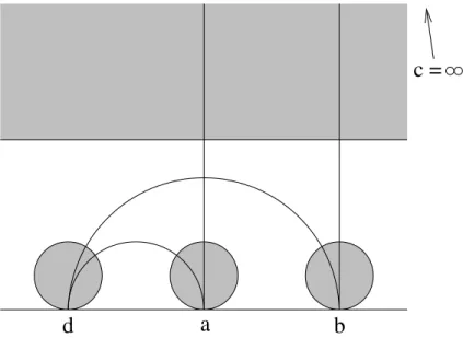
Letδ ⊂T1(S) denote a complete geodesic which is dense in both forward and backward time inT1(S). It follows that the set of all lifts ˜δofδ is dense inG( ˜S). Considering two disjoint lifts ˜δ1 =ad,δ˜2=bc, the set of bi-infinite geodesics that lie strictly between ˜δ1,δ˜2 is the set (a, b) ×(c, d) ⊂ G( ˜S) consisting of all the geodesics with one endpoint in the arc (a, b)⊂S1∞ and the other in the second arc (c, d)⊂S1∞; see Figure 5.
Density of the set of lifts ˜δ ofδ inG( ˜S) implies that µis determined by the set{µ((a, b)×(c, d))} over all (a, b)×(c, d) where ˜δ1 =ad,δ˜2 =bc are disjoint lifts ofδ. The proof of injectivity ofi∗ is then a consequence of the following claim, by taking→0.
Claim. Given disjoint lifts ˜δ1 = ad,δ˜2 = bc of δ and > 0, there exists α1, α2, α3, α4∈C(S) such that
µ((a, b)×(c, d))−i(α1, µ) +i(α2, µ)−i(α3, µ)−i(α4, µ) 2
< .
c
1 [α )2
[α )3 [α )4
δ2
τ1 τ2
δ1 d
b c
a a
d
b [α )
Figure 5: On the left: disjoint lifts ˜δ1,˜δ2ofδdefining a subset ofG( ˜S) of the form (a, b)×(c, d) ⊂G( ˜S) and the corresponding diagonal arcs ˜τ1,τ˜2. On the right: fundamental domains for (α1)∗, . . . ,(α4)∗ ∈π1(S) approximating the four geodesics
Proof of Claim. We sketch the idea; see [29] for the details.
Consider the geodesics ˜τ1 = ad,τ˜2 = bc as shown in Figure 5. Note that the set of geodesics (a, b)×(c, d) consists of precisely those geodesics that transversely intersect bothτ˜1 and ˜τ2, andneither δ˜1 nor ˜δ2. So, one is tempted to write
µ((a, b)×(c, d)) = µ(Eτ˜1) +µ(E˜τ2)−µ(E˜δ1)−µ(Eδ˜2) 2
However, the measures on the right are all infinite. For any > 0, we approximate the left-hand side to within > 0 by a formula similar to the right-hand side, where we replace each of the bi-infinite geodesics by appropriately chosen long, but finite length, subarcs [˜τi) ⊂τ˜i and [˜δi)⊂δ˜i, fori= 1,2. That is
µ((a, b)×(c, d))− µ(E[˜τ1)) +µ(E[˜τ2))−µ(E[˜δ
1))−µ(E[˜δ
2)) 2
< .
Density of δ in forward and backward time tells us that these arcs can be chosen so that the tangent vectors to these arcs (oriented from the “bottom”
to the “top” in the figure) at the endpoints are as close as we like to four vectors projecting to the same vector inT1(S). The arcs [˜τ1),[˜τ2),[˜δ1),[˜δ2) are therefore as close as we like to arcs [α1),[α2),[α3),[α4), respectively, which are fundamental domains for primitive closed geodesicsα1, α2, α3, α4,
respectively. With enough care, we can guarantee that the µ–measures of these also satisfy an inequality analogous to the previous one:
µ((a, b)×(c, d))− µ(E[α1)) +µ(E[α2))−µ(E[α3))−µ(E[α4)) 2
< . Applying Lemma 4.10 proves the claim.
Thus, i∗ is injective. The continuity of i∗ follows from continuity of i. To prove thati∗ is proper, letK ⊂RC≥0(S) be a compact set. Then for any curve α, there existsR >0 so thati−1∗ (K) is a closed subset of
CR(α) ={µ∈Curr(S)|i(α, µ)≤R}.
By Theorem 4.7,CR(α) is compact if αis a filling curve. Choosing α to be a filling curve, it therefore follows thati−1∗ (K) is compact, and hence i∗ is proper.
4.8 Liouville currents
For more on the results of this section, see [5]. Recall that G(H2) = (S1×S1\∆)/Z2,
where ∆ denotes the diagonal, andZ2 is the order-two group swapping the two coordinates. Given disjoint intervals [a, b] and [c, d] inS1, we define the Liouville measureof [a, b]×[c, d]⊂G(H2) as the modulus of the logarithm of the cross ratio of a, b, c, d:
L([a, b]×[c, d]) =
log
(a−c)(b−d) (a−d)(b−c)
. (4)
We refer to L as the Liouville current for H2. In the upper half-plane model ofH2, we can take (local) coordinates (x, y)∈R×R\∆⊂Rb×Rb\∆.
The current L is absolutely continuous with respect to Lebesgue measure dx dy and a simple calculation verifies that
L= dx dy (x−y)2.
In the disk model, with (eiα, eiβ)∈S1×S1\∆, one has L= dα dβ
|eiα−eiβ|2.


![Figure 3: The rule (x, [v]) 7→ ({a, b}, {c, d}) defines an identification between P T( ˜ S) and the subset of G( ˜ S) × G( ˜ S) consisting of those pairs of unoriented geodesics that are orthogonal to each other.](https://thumb-us.123doks.com/thumbv2/123dok_es/5734727.5460055/19.918.355.562.259.467/figure-defines-identification-subset-consisting-unoriented-geodesics-orthogonal.webp)