This is a post-peer-review, pre-copyedit version of an article published in International Journal of Life Cycle Assessment . The final authenticated version is available online at https://doi.org/10.1007/s11367-018-1443-y.
Global guidance on environmental life cycle impact assessment indicators: Impacts of climate
1
change, fine particulate matter formation, water consumption and land use
2
3
Olivier Jolliet1, Assumpció Antón2, Anne-Marie Boulay3,4, Francesco Cherubini5, Peter Fantke6, Annie
4
Levasseur3, Thomas E. McKone7, Ottar Michelsen8, Llorenç Milà i Canals9, Masaharu Motoshita10,
5
Stephan Pfister11, Francesca Verones5, Bruce Vigon12, Rolf Frischknecht13
6
7
Corresponding author: Olivier Jolliet, [email protected], Tel. +1 (734) 647 0394, Fax. +1 (734) 936
8
7283
9
10
1 Environmental Health Sciences, School of Public Health, University of Michigan, Ann Arbor, MI,
11
USA.
12
2IRTA, Institute for Food and Agricultural Research and Technology, Cabrils, Barcelona, Spain
13
3CIRAIG, Department of Chemical Engineering, Polytechnique Montreal, Montreal, Canada.
14
4LIRIDE, Sherbrooke University, Sherbrooke, Canada
15
5Industrial Ecology Programme, Department of Energy and Process Engineering, Norwegian University
16
of Science and Technology, Trondheim, Norway
17
6 Department of Management Engineering, Quantitative Sustainability Assessment Division, Technical
18
University of Denmark, Kgs. Lyngby, Denmark.
19
7School of Public Health, University of California, Berkeley, CA, USA
20
8NTNU Sustainability, Norwegian University of Science and Technology, Trondheim, Norway
21
9Economy Division, United Nations Environment Programme, Paris, France.
22
10National Institute of Advanced Industrial Science and Technology, Tsukuba, Japan
23
11ETHZ - Swiss Federal Institute of Technology - Zurich, Zurich, Switzerland
24
12SETAC, Pensacola, FL, USA.
25
13treeze Ltd., Uster, Switzerland.
26
27
28
1. Abstract
29
Purpose Guidance is needed on best suited indicators to quantify and monitor the man-made impacts on
30
human health, biodiversity and resources. Therefore, the UNEP-SETAC Life Cycle Initiative initiated
31
a global consensus process to agree on an updated overall life cycle impact assessment (LCIA)
32
framework and to recommend a non-comprehensive list of environmental indicators and LCIA
33
characterization factors for 1) climate change, 2) fine particulate matter impacts on human health, 3)
34
water consumption impacts (both scarcity and human health), and 4) land use impacts on biodiversity.
35
Method The consensus building process involved more than 100 world-leading scientists in task forces
36
via multiple workshops. Results were consolidated during a one week Pellston WorkshopTM in January
37
2016 leading to the following recommendations.
38
Results
39
LCIA framework: The updated LCIA framework now distinguishes between intrinsic, instrumental
40
and cultural values to assess, with DALY to characterize damages on human health and with measures
41
of vulnerability included to assess biodiversity loss.
42
Climate change impacts: Two complementary climate change impact categories are recommended: a)
43
The Global Warming Potential 100 years (GWP 100) represents shorter term impacts associated with
44
rate of change and adaptation capacity, and b) the Global Temperature change Potential 100 years (GTP
45
100) characterizes the century-scale long term impacts, both including climate-carbon cycle feedbacks
46
for all climate forcers.
47
Fine particulate matter (PM2.5) health impacts: Recommended characterization factors (CFs) for
48
primary and secondary (interim) PM2.5 are established, distinguishing between indoor, urban and rural
49
archetypes.
50
Water consumption impacts: CFs are recommended, preferably on monthly and watershed levels, for
51
two categories: a) The water scarcity indicator “AWARE” characterizes the potential to deprive human
52
and ecosystems users and quantifies the relative Available WAter REmaining per area once the demand
53
of humans and aquatic ecosystems has been met, and b) the impact of water consumption on human
54
health assesses the DALYs from malnutrition caused by lack of water for irrigated food production.
55
Land use impacts: CFs representing global potential species loss from land use are proposed as interim
56
recommendation suitable to assess biodiversity loss due to land use and land use change in LCA hotspot
57
analyses.
58
Conclusions The recommended environmental indicators may be used to support the UN Sustainable
59
Development Goals in order to quantify and monitor progress towards sustainable production and
60
consumption. These indicators will be periodically updated, establishing a process for their stewardship.
61
Keywords
62
LCIA framework, Climate change, Fine particulate, Human health, Water scarcity, Water consumption,
63
Land use.
64
2. Introduction and goal of the harmonisation process
65
The current environmental pressure and, especially, its reduction according to the UN Sustainable
66
Development Goals (United Nations 2015) in the coming years require the development of
67
environmentally sustainable products and services. Because markets and supply chains are increasingly
68
globalised, harmonised guidelines are needed on how to quantify the environmental life cycle impacts
69
of products and services. In particular, guidance is needed on which quantitative and life cycle based
70
indicators are best suited to quantify and monitor the man-made impacts on human health, biodiversity,
71
water resources, etc. The ongoing developments in the application of life cycle assessment (LCA) to
72
Product Environmental Footprint and to a wide range of products, calls for not only providing
73
recommendations to method developers, but also to provide recommended globally applicable
74
indicators that can then be used in such footprints within comprehensive life cycle impact assessment
75
(LCIA) approaches. Following multiple open consultations and workshops in multiple continents
76
(Jolliet et al. 2014), stakeholders in industry, public policy and academia thus agreed on the need for
77
consensus and global guidance on environmental LCIA indicators.
78
A series of complementary initiatives for LCIA consensus building have taken place since the early
79
1990s, striving towards providing recommendations and guidance for the development and use of LCIA
80
methods. Two rounds of SETAC working groups led to category-specific recommendations for
81
developing LCIA impact indicators (Udo de Haes et al. 2002), taking advantage of broader consensus
82
efforts, such as those led by the Intergovernmental Panel on Climate Change for climate change issues.
83
The LCIA program of the phase I and phase II of the UNEP-SETAC Life Cycle Initiative developed a
84
combined midpoint-damage framework (Jolliet et al. 2004), and provided further recommendations for
85
multiple impact categories. The UNEP-SETAC scientific consensus toxicity model was then developed
86
and endorsed to estimate ecotoxicity and human toxicity impacts in LCA (Rosenbaum et al. 2008; Westh
87
et al. 2015). In parallel, more emphasis was given to better frame resource-related categories, especially
88
for land use (Milà i Canals et al. 2007) and water use, with the launch of a Water Use in LCA working
89
group, WULCA (Köhler 2007). Since the launch of phase I of the initiative and the publication of its
90
framework, several developments have been and are being carried out for developing worldwide
91
applicable methods, with spatially differentiated impact indicators, at midpoint level (Hauschild et al.
92
2011 and 2013) and damage level (Bulle et al. 2016; Frischknecht et al. 2013; Huijbregts et al. 2014and
93
2017; Itsubo and Inaba 2010). These developments now need to be accounted for in a global consensus
94
building process.
95
To answer these needs, Phase III of the UNEP-SETAC Life Cycle Initiative launched a flagship project
96
to provide global guidance and build consensus on environmental LCIA indicators. Initial workshops in
97
Yokohama in 2012 and in Glasgow 2013 as well as a stakeholder consultation scoped this flagship
98
project (Jolliet et al. 2014), focusing the effort in a first stage on a) impacts of climate change, b) fine
99
particulate matter health impacts, c) water consumption and d) land use, plus e) crosscutting issues and
100
f) LCA-based footprints. For each of the impact categories, the main objective of the flagship project is
101
four-fold: (1) To describe the impact pathway and review the potential indicators. (2) Based on well-
102
defined criteria, to select the best-suited indicator or set of indicators, identify or develop the method to
103
quantify them on sound scientific basis, and provide characterization factors with corresponding
104
uncertainty and variability ranges. (3) To apply the indicators to a common LCA case study to illustrate
105
its domain of applicability. (4) To provide recommendations in term of indicators, status and maturity
106
of the recommended factors, applicability, link to inventory databases, roadmap for additional tests and
107
potential next steps. The scope of the work is not to cover comprehensively all relevant impact categories
108
and the list of resulting impact category indicators should not be interpreted as a sufficient or complete
109
list of impacts to address in LCA.
110
This paper presents the consensus building process and scientific approach retained, as well as the
111
indicators selected and recommendations reached for the above-described selected impact categories
112
and crosscutting issues. The first section describes the process and criteria used to select the
113
recommended indicators. The second section presents the updated LCIA framework. The next sections
114
describe the selected characterization factors and the main recommendations for each of the four impact
115
categories considered. The paper ends by applying the recommended indicators to a rice case study,
116
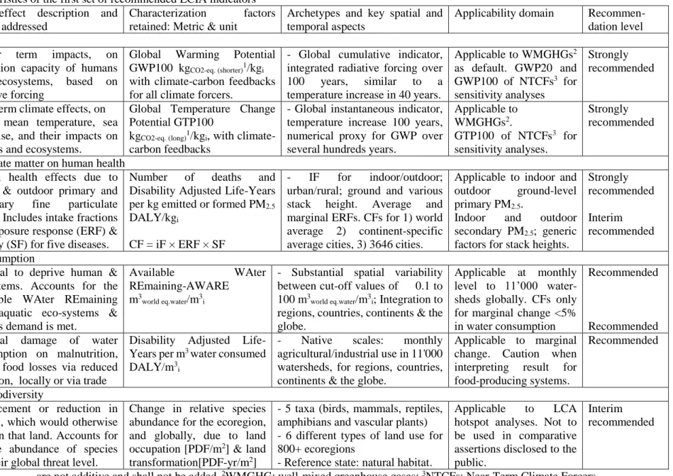
followed by conclusions and outlook that addresses potential concerns that such consensus processes
117
may raise (Huijbregts, 2014). A more comprehensive description of the process and its outcome is
118
further detailed in the first assessment report on LCIA guidance (Frischknecht and Jolliet 2016).
119
3. Process and recommendation criteria
120
Process: To achieve the goals of the LCIA harmonisation project, following open calls for interest and
121
search for category specific specialists, task forces were set up involving more than 100 world-leading
122
domain experts and LCA scientists, organized in impact category specific task forces (TFs) and
123
complemented by a TF on crosscutting issues. Multiple topical workshops and conferences were
124
organised by each individual TF to first scope the work and then develop scientifically robust state-of-
125
the-art indicators suitable for a global consensus (Boulay et al. 2015c; Cherubini et al. 2016; Curran et
126
al. 2016; Fantke et al. 2015; Hodas et al. 2016; Levasseur et al. 2016; Teixeira et al. 2016). This was
127
followed by two overarching workshops and stakeholder meetings in Basel 2014 and in Barcelona 2015
128
to address specific critical crosscutting issues and collect feedback from multiple stakeholders. Section
129
S1 of the supporting information further details the multiple workshops and communications carried out
130
in each task force. Additionally, an LCA case study on the production and consumption of rice common
131
to all TFs (Frischknecht et al. 2016) was developed to test the recommended impact category indicators
132
selected in the harmonisation process and further help to ensure their practicality.
133
This first part of the consensus-finding process ended with a one week Pellston WorkshopTM. According
134
to the standard operating procedures for SETAC-supported Pellston WorkshopsTM, a steering committee
135
was first appointed by the International Life Cycle Panel of the Life Cycle Initiative, with diverse
136
members from government, academia/NGO and industry (steering committee composition in section S2
137
of supplementary information). The steering committee selected 40 invited experts and stakeholders
138
from industry, academia, government and NGOs originating from 14 different countries, both among
139
and outside the task forces to ensure a broad worldwide representativeness (see list of additional
140
workshop participants in acknowledgments). The workshop took place in Valencia, Spain, from 24 to
141
29 January 2016 to make recommendations on environmental indicators for each of the considered
142
impact category. This paper summarizes decisions reached at this workshop, complemented by work of
143
the specific TFs.
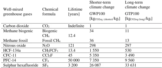
144
Guiding principles for harmonisation: Building on the earlier work and process by Hauschild et al.
145
(2011 and 2013), the following global guiding principles were identified and applied in the LCIA
146
indicator harmonisation process: Environmental relevance to ensure that the recommended indicators
147
address environmentally important issues; completeness to ensure they cover a maximum achievable
148
part of the corresponding environmental issue with global coverage; scientific robustness to ensure they
149
follow state-of-the-art knowledge and evidence rather than subjective assumptions; documentation and
150
transparency to ensure that the recommended indicators are accessible and reproducible; applicability
151
and level of experience to ensure that the recommended approaches can easily be implemented and
152
applied in LCA databases, and have proven their practicality in a number of sufficiently diverse LCA
153
case studies; and stakeholder acceptance to ensure that the indicators meet the needs and requirements
154
of science and non-governmental organisations and of decision makers in industry and governments.
155
Starting from a generic checklist, criteria were first customized for the considered impact category.
156
Existing impact category indicators were then systematically evaluated and compared against these
157
evaluation criteria, leading to white papers as inputs to the Pellston workshop. The scope of this
158
harmonisation work was not to provide a complete set of environmental LCIA indicators nor to create
159
a new and comprehensive LCIA method. The selection of impact categories in the present report was
160
primarily based on potential for global consensus (Jolliet et al. 2014) and is not to be interpreted as an
161
implicit expression of preference on these topics over others.
162
Levels of recommendations: The recommendations presented in this paper are the result of consensus-
163
finding processes based on objectively supportable evidence, with the aim to ensure consistency and
164
practicality. They however do not necessarily reflect unanimous agreement and the body of experts
165
assigns levels of support for a practice or indicator, according to the workshop process principles and
166
rules. These levels are stated by consistently applying the terminology of “strongly recommended”,
167
“recommended”, “interim recommended”, and “suggested or advisable”.
168
169
4. LCIA framework and modelling guidance
170
4.1 Framework and damage categories
171
A consistent framework is key to ensure that new developments and findings can be integrated into
172
LCIA in a way that makes environmental impact category indicators compatible. Building on the earlier
173
LCIA framework of the UNEP-SETAC Life Cycle Initiative (Jolliet et al. 2004), Verones et al. (2017)
174
proposed an updated framework, distinguishing three different kinds of values: 1) Intrinsically valued
175
systems that have a value by virtue of their existence (e.g. ecosystem quality as well as human health),
176
2) instrumentally valued systems, which have a clear utility to humans (natural resources, ecosystem
177
services and socio-economic assets), and 3) culturally valued systems which have a value to humans by
178
virtue of artistic, aesthetic, recreational, or spiritual qualities. These cultural values have so far rarely
179
been assessed in LCA, but could be included in the future.
180
Each environmental intervention (elementary flow) may have impacts on several of these values and
181
impact categories that can be determined and reported separately.
182 183
In this updated LCIA framework , impact characterization models link the life cycle inventory results
184
to impacts at midpoint level or at damage level. Impact categories at damage level are available on a
185
disaggregated level (e.g. climate change or land use impacts), or can be aggregated into overarching
186
areas of protection. Conversion factors that provide the linkage between midpoint level and damage
187
level impacts may be spatially variable and therefore non-constant. Weighting or normalization of
188
damage category scores are optional steps distinct from damage modelling.
189
It is acceptable, though not promoted, that, for the case that no relevant midpoint impact indicator can
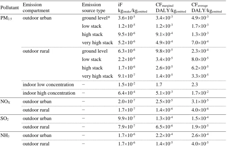
190
be identified along the impact pathway, proxy indicators can be designed, which are not defined along
191
an impact pathway itself, such as for example water scarcity indicators (section 4.3 below). These
192
proxies need to be thoroughly justified, clearly labelled and documented, in order to avoid confusion.
193
4.2 Damage category specific recommendations
194
The following recommendations are made for the indicators pertaining the three presently operational
195
damage categories, for human health, ecosystem quality and natural resources.
196
Human health is an area of protection that deals with the intrinsic values of human health, addressing
197
both their mortality and morbidity. It is recommended to continue using Disability-Adjusted Life Years
198
(DALYs) in LCIA for human health, as proposed and motivated by Fantke et al. (2015), following the
199
current Global Burden of Disease (GBD) approach (Forouzanfar et al. 2015) and not including age
200
weighting nor discounting. It is also recommended to transparently document the different components
201
of a DALY separately (e.g., the years of life lost-YLL, and the Years Lived with Disability-YLD).
202
Ecosystem quality is an area of protection dealing with terrestrial, freshwater, and marine ecosystems
203
and biodiversity, focusing on their intrinsic value. It is recommended to characterize ecosystems and/or
204
species in a way that takes resilience, rarity and recoverability into account. It is recommended that the
205
unit at the damage level should be based on “potentially disappeared fraction (PDF) of species” (e.g.
206
global or local PDF, PDF-m2-yr or PDF-m3-yr). Any method addressing biodiversity that includes units
207
that are convertible to PDF related metrics is recommended to describe and report the conversion factors.
208
It is recommended to develop CFs at local, regional and global levels, to reflect losses in local and
209
regional ecosystem functionality and global extinction. We emphasize that impacts quantified at global
210
level (i.e. species are completely lost from the Earth) cannot be directly compared with local or regional
211
impacts (i.e. species are only extinct in a certain part of the world); thus method developers need to
212
report very explicitly at which level their model was developed.
213
Natural resources are material and non-material assets occurring in nature that are at some point in time
214
deemed useful for humans (Sonderegger et al. 2017). Ecosystem services are instrumental values of
215
ecosystems and, therefore, impacts on ecosystem services are different from impacts on ecosystem
216
quality, which represents an intrinsic value. It is recommended that method developers also address the
217
instrumental value of natural resources and ecosystem services when developing impact indicators and
218
CFs, considering the different nature of resources, i.e. stocks, funds and flows.
219
A number of recommendations are further detailed in Verones et al. (2017), regarding transparent
220
reporting on reference states, spatial differentiation, and addressing uncertainties, as well as
221
normalization and weighting.
222
5. Selected indicators, characterization factors and main recommendations
223
This section provides the background, the description of selected indicators and a summary of the
224
calculation methods, a list of selected characterization factors and the main recommendations for each
225
of the four impact categories considered. The full list of characterization factors is available for
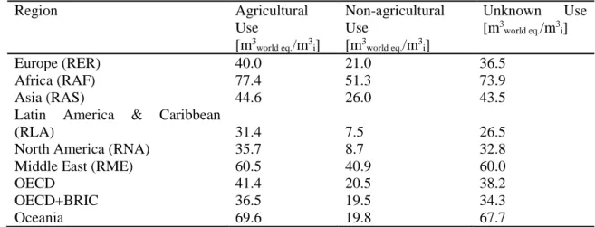
226
download on the UNEP-SETAC life Cycle Initiative website
227
(http://www.lifecycleinitiative.org/applying-lca/lcia-cf/).
228
Table 1 Main characteristics of the first set of recommended LCIA indicators
229
Impact category
& subcategory
Cause-effect description and impact addressed
Characterization factors retained: Metric & unit
Archetypes and key spatial and temporal aspects
Applicability domain Recommen- dation level a) Climate change impacts
a1) Climate Change
Shorter-term
Shorter term impacts, on adaptation capacity of humans and ecosystems, based on radiative forcing
Global Warming Potential GWP100 kgCO2-eq. (shorter)1/kgi
with climate-carbon feedbacks for all climate forcers.
- Global cumulative indicator, integrated radiative forcing over 100 years, similar to a temperature increase in 40 years.
Applicable to WMGHGs2 as default. GWP20 and GWP100 of NTCFs3 for sensitivity analyses
Strongly recommended
a2) Climate Change
Long-term
Long-term climate effects, on global mean temperature, sea level rise, and their impacts on humans and ecosystems.
Global Temperature Change Potential GTP100 kgCO2-eq. (long)1/kgi, with climate- carbon feedbacks
- Global instantaneous indicator, temperature increase 100 years, numerical proxy for GWP over several hundreds years.
Applicable to WMGHGs2.
GTP100 of NTCFs3 for sensitivity analyses.
Strongly recommended
b) Impacts of fine particulate matter on human health Health impacts
of fine particles
Human health effects due to indoor & outdoor primary and secondary fine particulate matter. Includes intake fractions (iF),exposure response (ERF) &
severity (SF) for five diseases.
Number of deaths and Disability Adjusted Life-Years per kg emitted or formed PM2.5
DALY/kgi
CF = iF × ERF × SF
- IF for indoor/outdoor;
urban/rural; ground and various stack height. Average and marginal ERFs. CFs for 1) world average 2) continent-specific average cities, 3) 3646 cities.
Applicable to indoor and outdoor ground-level primary PM2.5.
Indoor and outdoor secondary PM2.5; generic factors for stack heights.
Strongly recommended Interim recommended c) Impacts of Water Consumption
c1) Water
scarcity
Potential to deprive human &
ecosystems. Accounts for the Available WAter REmaining once aquatic eco-systems &
humans demand is met.
Available WAter
REmaining-AWARE m3world eq.water/m3i
- Substantial spatial variability between cut-off values of 0.1 to 100 m3world eq.water/m3i; Integration to regions, countries, continents & the globe.
Applicable at monthly level to 11’000 water- sheds globally. CFs only for marginal change <5%
in water consumption
Recommended
Recommended c2) Impacts of
water
consumption on human health
Potential damage of water consumption on malnutrition, due to food losses via reduced irrigation, locally or via trade
Disability Adjusted Life- Years per m3 water consumed DALY/m3i
- Native scales: monthly agricultural/industrial use in 11'000 watersheds, for regions, countries, continents & the globe.
Applicable to marginal change. Caution when interpreting result for food-producing systems.
Recommended
d) Land use impacts on biodiversity Potential species
loss due to land occupation &
transformation
Displacement or reduction in species, which would otherwise exist on that land. Accounts for relative abundance of species and their global threat level.
Change in relative species abundance for the ecoregion, and globally, due to land occupation [PDF/m2] & land transformation[PDF-yr/m2]
- 5 taxa (birds, mammals, reptiles, amphibians and vascular plants) - 6 different types of land use for 800+ ecoregions
- Reference state: natural habitat.
Applicable to LCA hotspot analyses. Not to be used in comparative assertions disclosed to the public.
Interim recommended
1 kgCO2-eq.(shorter) and kgCO2-eq.(long) are not additive and shall not be added. 2WMGHG: well-mixed greenhouse gases; 3NTCFs: Near-Term Climate Forcers
230
5.1 Climate change
231
5.1.1 Background and scope
232
LCA studies quantify the climate change impacts of greenhouse gas emissions due to human activities
233
by aggregating them into a common unit, e.g. CO2-equivalent (Hellweg & Milà i Canals 2014). Global
234
Warming Potential (GWP, IPCC 2007) has been the default metric used in LCIA since its first
235
publication in 1990 and none of the substantial advancements in climate science or new metrics (e.g.
236
Global Temperature Change Potential – GTP, Shine et al. 2005) have been considered. Two main
237
challenges were addressed towards more comprehensive LCIA indicators: a) how to best characterize
238
gases with lifetimes ranging from a few years for methane (CH4), up to several hundreds or thousands
239
of years for well-mixed greenhouse gases (WMGHG) such as carbon dioxide or CFCs, and b) how to
240
consider the new climate science developments on climate-carbon cycle feedbacks (the changing climate
241
influencing itself, e.g. the rates of soil respiration and photosynthesis), and on the contributions from
242
Near-Term Climate Forcers (NTCFs, like ozone precursors and aerosols such as black carbon). Climate
243
change impacts from human-induced albedo changes were not considered.
244
5.1.2 Description of selected indicators
245
a) Selected indicators (Table 1a): There is no single metric that can adequately assess the different
246
contributions of climate forcing agents to both the rapid shorter-term temperature changes and the long-
247
term temperature increases that are associated with different types of damages. It is therefore
248
recommended to adopt two distinct and complementary subcategories based on two separate indicators:
249
1) Shorter-term climate change, addressing shorter-term environmental and human health consequences
250
from the rate of climate change (over next decades, e.g., lack of human and ecosystems adaptation),
251
using GWP 100 as indicator. By explicitly accounting for all the forcing of an emission until the time
252
horizon, GWP100 captures the cumulative effects of climate pollutants that contribute to the rate of
253
warming. As it is numerically close to GTP40 (Allen et al. 2016), it can be interpreted as a proxy for
254
temperature impacts within about four decades, a time scale markedly shorter than that of GTP100.
255
2) Long-term climate change impacts, reflecting the long-term effects from climate change (over next
256
centuries, e.g., future temperature stabilization, sea level rise), using GTP 100 as indicator. GTP100 is
257
an instantaneous indicator measuring the potential temperature rise still occurring 100 years after
258
emission. Its numerical values are similar to GWP with a time horizon of several centuries, which would
259
have also been a suitable indicator to reflect long-term effects from climate change. However, the IPCC
260
does not provide GWP values for such long time horizons, since modeling too far in the future would
261
lead to very high uncertainties.
262
Sensitivity analysis: Given the high uncertainty ranges associated with the CFs for NTCFs, these should
263
only be considered in a sensitivity analysis using the range of values for each species. Results can be
264
shown by taking the CFs representing a best case (using the lower end of the range) and a worst case
265
(using the upper end of the range) scenario. It is also recommended to use GWP20 in a sensitivity
266
analysis for assessing the dependency of the results on an indicator based on very short term climate
267
change effects.
268
b) Calculation method: The GWP from the IPCC 5th Assessment Report (Myhre et al. 2013, Joos et
269
al. 2013) are produced from models that give the temporal evolution of radiative forcing in response to
270
an instantaneous emission of a climate forcer. For CO2 the impulse response function consists of three
271
terms governed by distinct decay time constants, and one time-invariant constant term that represents a
272
variety of carbon cycle processes operating on a range of time scales (Joos et al. 2013). Simpler models
273
are used for non-CO2 climate forcers with simple exponential decays, accounting for indirect effects for
274
CH4 and N2O. The GTP are obtained from models yielding the temporal evolution of global-mean
275
temperature change due to changes in radiative forcing. These models are based on a short and a longer
276
time constant that are calibrated using more complex models (Boucher and Reddy 2008). Further
277
technical details can be found in Section 8.SM.11 of IPCC 5th AR, as well as in the two publications of
278
the climate change TF (Levasseur et al. 2016; Cherubini et al. 2016).
279
c) Characterization factors: Table 2 provides the recommended values for a subset of the main
280
greenhouse gases contributing to climate change. Additional values for GWP20 and NTCFs for
281
sensitivity studies can be found in the climate change chapter of the full report (Frischknecht and Jolliet
282
2016, Chapter 3). Compared to earlier Global Warming potentials, the improvement of models and the
283
inclusion of climate-carbon feedbacks for all climate forcers leads to an increased value of the shorter–
284
term indicator GWP100 for methane from 25 (IPCC 2007) to 34 kgCO2-eq.(shorter)/kgCH4. When considering
285
the long-term indicator GTP100, CH4 impact is smaller relative to CO2 and amounts to 11 kgCO2-
286
eq.(long)/kgCH4. The factors for fossil methane include the degradation of fossil methane into CO2 and thus
287
are higher by 2 kgCO2-eq.(long)/kgCH4 for both indicators compared to the factor for biogenic methane. kgCO2-
288
eq.(shorter) and kgCO2-eq.(long) are not additive and shall not be added, thus the indication in parentheses, i.e.
289
(shorter) and (long).
290
291
Table 2 IPCC Characterization factors for selected greenhouse gases, representing shorter-term
292
(GWP100) and long-term (GTP100) climate change impacts, according to Myhre et al. (2013, Table
293
8.A.1).
294 295
Well-mixed greenhouse gases
Chemical formula
Lifetime [years]
Shorter-term climate change
Long-term climate change GWP100
[kgCO2eq. (shorter)/kgi]
GTP100
[kgCO2eq.(long)/kgi]
Carbon dioxide CO2 Indefinite 1 1
Methane biogenic Biogenic
CH4 12.4
34 11
Methane fossil Fossil CH4 36 13
Nitrous oxide N2O 121 298 297
HCF-134a CH2FCF3 13.4 1 550 530
CFC-11 CCl3F 45 5 350 3 490
PFC-14 CF4 50 000 7 350 9 560
Sulphur hexafluoride SF6 3 200 26 087 33 631
296
CFs for Near-Term Climate Forcers and GWP20 are available for download on the UNEP-SETAC life
297
Cycle Initiative website (http://www.lifecycleinitiative.org/applying-lca/lcia-cf/) to perform the
298
recommended sensitivity studies and assess very short-term climate change effects.
299
5.1.3 Recommendation and applicability
300
It is strongly recommended to use GWP100 for the shorter-term impact category related to the rate of
301
temperature change, and GTP100 for the long-term impact category related to the long-term temperature
302
rise for WMGHGs. Based on the IPCC AR5 recommendations, it is recommended to consistently use
303
the characterization factors that include the climate-carbon cycle feedbacks for both non-CO2 GHGs and
304
CO2. For the shorter-term climate effects, a sensitivity analysis may also include results from NTCFs
305
and may apply GWP20 (in addition to GWP100) as CFs.
306
The use of two complementary climate change impact subcategories in LCA is an element of novelty
307
compared to the traditional practice, which is based on the use of a single climate change indicator
308
(usually GWP100). The proposed refinement will certainly require updates of CFs in common database
309
and software providers, and the availability of characterization factors in the IPCC 5th AR can make
310
this transition easy. Modest adaptation efforts from practitioners will ensure an important step forward
311
in the robustness and relevance of climate change impact assessment in LCA.1 For sensitivity analysis
312
including NTCFs, it is also recommended to complement life cycle inventory databases with explicit
313
1 One participant expressed in a minority statement its concerns regarding the implications of recommending two impact categories for climate change for practical applications of LCA, with the risk that different climate change labels used on products present divergent information.
data on black carbon and organic carbon emissions, which are currently aggregated within particulate
314
matter emissions.
315
5.2 Fine particulate matter impacts on human health
316
5.2.1 Background and scope
317
A number of health studies, in particular the global burden of disease (GBD) project series (Lim et al.
318
2012), reveal the significant disease burden posed by fine particulate matter (PM2.5) exposures indoors
319
(household and occupational buildings air) and outdoors (ambient urban and rural air) to the world
320
population. However, clear guidance is currently missing on how health effects associated with PM2.5
321
exposure can be consistently included in LCIA (Fantke et al. 2015). This section provides a consistent
322
modelling framework elaborated by multiple world experts for calculating characterization factors for
323
indoor and outdoor emission sources of primary PM2.5 and secondary PM2.5 precursors.
324
5.2.2 Description of selected indicators
325
a) Selected framework and indicators (Table 1b): The general framework extends earlier work from
326
the UNEP-SETAC life cycle initiative on the health effects from PM2.5 exposure (Humbert et al. 2011,
327
Humbert et al. 2015) and includes the combination of three factors and metrics, characterizing exposure,
328
health response and severity:
329
Exposure: The intake fraction iF [kginhaled/kgemitted], expressed as the fraction of an emitted mass of PM2.5
330
or precursor ultimately taken in as PM2.5 by the total exposed population (Bennett et al. 2002), was
331
selected as the exposure metric for both indoor and outdoor primary PM2.5 and secondary PM2.5
332
precursor emissions. Emission source types indoors and outdoors can be associated with a specific iF.
333
Such an iF is easier to interface and combine at the level of human exposure than a field of indoor or
334
ambient concentrations over a certain distance around the considered emission sources.
335
Exposure-response: The exposure-response slope factor ERF [deaths/ kginhaled] represents the change in
336
all-cause mortality (or in specific disease endpoints) per additional population intake dose unit. This
337
exposure-response slope is determined based on the non-linear integrated exposure-response model
338
developed by Burnett et al. (2014) to support the 2010 GBD analysis. It synthesizes effect estimates
339
from eight cohort studies of ambient air pollution, combined with effect estimates from indoor studies
340
at much higher levels of exposure (second-hand smoke and active smoking, indoor air pollution from
341
cooking).
342
Severity: The severity factor, SF [DALYs/death], represents the change in human health damage
343
expressed as disability-adjusted life years per death, as summarized in the GBD (Lim et al. 2012;
344
Forouzanfar et al. 2015). The health metric chosen for exposure to PM2.5 indoors and outdoors is the
345
Disability-Adjusted Life Year (DALY) without age weighting and without discounting (see Section
346
4.2), summing up Years of Life Lost (YLL) and Years Lived with Disability (YLD). The latter includes
347
a weighting factor describing the quality of life during the period of disability (Murray 1994).
348
The resulting characterization factors, CF [DALY/kgemitted], are then determined as the product of these
349
three metrics:
350
SF ERF iF
CF (1)
351
b) Calculation method - spatial/temporal differentiation: Data for calculating the intake fraction iF
352
are mainly based on Apte et al. (2012) for outdoor urban environments and on Brauer et al. (2016) for
353
outdoor rural environments. These outdoor urban and rural/remote area archetypes are further
354
disaggregated to account for ground level, low stack, high stack, and very high stack emissions. We
355
distinguish outdoor archetypes at three levels of detail (Fantke et al. 2017): At generic level 1, default
356
iF values are calculated reflecting a population weighted average intake fraction. At intermediary level
357
2, iF are provided for continent-specific average cities, to represent urban areas for a continental and
358
sub-continental regions. The characteristics of each of the 3646 cities with more than 100000 inhabitants
359
are used in the detailed level 3 iF calculation. The basic ground work for calculating iF for different
360
indoor source environments is provided by Hodas et al. (2015). The considered archetypes differentiate
361
high, medium and low ventilation rates, further subdivided into with and without PM2.5 filtration, and
362
into indoor spaces with high, medium and low occupancy. The coupled indoor-outdoor emission-to-
363
exposure framework is available as a spreadsheet and fully described in Fantke et al. (2017).
364
The ERF slope for total mortality is determined at the working point for exposure to PM2.5 in indoor and
365
outdoor environments based on the supralinear integrated risk function of Burnett et al. (2014), with
366
data for outdoor background mortality rates based on Apte et al. (2015). The marginal slope at the
367
working point is provided when small changes are expected, and the average slope between the working
368
point and the minimum risk is given for large variations.
369
The typical time scale considered are a few days or weeks for fate and exposure - to assess cumulative
370
exposures, and decades or lifetime for exposure-response functions - to account for long-term mortality.
371
c) Characterization factors: Table 3 provides the global generic level 1 recommended default values.
372
Marginal PM2.5 CFs vary by up to 5 orders of magnitude, ranging from 1.4×10⁻⁵ DALY/kgemitted for
373
outdoor rural high stack emissions up to 1.7 DALY/kgemitted for indoor emissions in low background
374
PM2.5 concentration situations.
375
376
Table 3 Summary of default intake fractions (based on Fantke et al. 2017) and characterization factors
377
for human health impacts of primary PM2.5 emissions and of secondary PM2.5 precursor emissions,
378
applying the marginal and the average exposure response slope at working point.
379 380
Pollutant Emission compartment
Emission source type
iF
kgintake/kgemitted
CFmarginal
DALY/kgemitted
CFaverage
DALY/kgemitted
PM2.5 outdoor urban ground level* 3.6×10⁻⁵ 3.4×10⁻³ 4.9×10⁻³
low stack 1.2×10⁻⁵ 1.2×10⁻³ 1.7×10⁻³
high stack 9.5×10⁻⁶ 9.1×10⁻⁴ 1.3×10⁻³
very high stack 5.2×10⁻⁶ 4.9×10⁻⁴ 7.0×10⁻⁴
outdoor rural ground level 6.3×10⁻⁶ 9.8×10⁻⁵ 2.3×10⁻⁴
low stack 2.2×10⁻⁶ 3.4×10⁻⁵ 8.0×10⁻⁵
high stack 1.7×10⁻⁶ 2.6×10⁻⁵ 6.2×10⁻⁵
very high stack 9.1×10⁻⁷ 1.4×10⁻⁵ 3.3×10⁻⁵
indoor low concentration − 1.5×10⁻² 1.7 2.3
indoor high concentration − 6.4×10⁻⁴ 5.1×10⁻³ 1.7×10⁻²
NOX outdoor urban − 2.0×10⁻⁷ 2.5×10⁻⁵ 3.1×10⁻⁵
outdoor rural − 1.7×10⁻⁷ 1.4×10⁻⁶ 4.0×10⁻⁶
SO2 outdoor urban − 9.9×10⁻⁷ 1.3×10⁻⁴ 1.5×10⁻⁴
outdoor rural − 7.9×10⁻⁷ 6.5×10⁻⁶ 1.9×10⁻⁵
NH3 outdoor urban − 1.7×10⁻⁶ 2.2×10⁻⁴ 2.6×10⁻⁴
outdoor rural − 1.7×10⁻⁶ 1.4×10⁻⁵ 4.0×10⁻⁵
*Reference emission scenario.
381
5.2.3 Recommendation and applicability
382
Overarching recommendations are summarized and prioritized below:
383
Strong recommendations: The intake fraction metric is strongly recommended to capture source-
384
receptor relationships for indoor and outdoor primary PM2.5, using the archetypes of Table 3 to
385
differentiate exposure and where possible city-specific intake fractions to capture the large interurban
386
variability. Proper application of the well-vetted exposure-response models for assessing both total
387
mortality and disease-specific DALYs requires to account for background PM2.5 exposure.
388
Recommendations: it is recommended that the LCA practitioner qualitatively and (when possible)
389
quantitatively characterizes variability and uncertainty, based on information given in Hodas et al.
390
(2016) and Fantke et al. (2017). Interim Recommendations: Using current literature values for secondary
391
PM2.5 formation indoors and outdoors and generic factors for low, high, and very high stack emissions
392
based on the use of ground level emissions (Humbert et al. 2011) are interim recommendations that can
393
be readily used by practitioners as implemented in Fantke et al. (2017).
394
The provided factors capture the global central values for CFs but also allow for exploration of
395
variability among subcontinental regions and cities, via a stepwise application from global averages to
396
subcontinent and city specific CFs.
397
5.3 Water scarcity index
398
5.3.1 Background and scope
399
Water consumption can lead to deprivation and impacts on human health and ecosystems quality and is
400
a relevant impact category to integrate in LCA, as framed by previous work of the WULCA working
401
group Bayart et al. (2010), Kounina et al. (2013) and Boulay et al. (2015a,b,c). According to the ISO
402
water footprint standard (ISO 2014), water scarcity is the “extent to which demand for water compares
403
to the replenishment of water in an area, such as a drainage basin”. While most existing water scarcity
404
indicators were defined to be applicable either for human health or ecosystems impacts, there is a need
405
for a generic water scarcity indicator, which explicitly represents the potential to deprive both human
406
and ecosystems users.
407
This section describes the generic consensus scarcity index to assess potential impacts associated with
408
a marginal water consumption, addressing the following question: What is the potential to deprive
409
another user (human and ecosystems) when consuming water in a considered area?
410
5.3.2 Description of selected indicators
411
a) Selected indicators (Table 1c): Multiple indicators (Withdrawal-to-Availability, Consumption-to-
412
Availability, corrected Demand-to-Availability and Availability-minus-Demand) were first compared
413
and analysed based on the following pre-defined criteria: stakeholders acceptance, robustness with
414
closed basins, main normative choice and physical meaning. Based on this comparison, the inverse of
415
the Availability-minus-Demand (1/AMD) has been retained as a basis for the scarcity indicator method,
416
called Available WAter REmaining – AWARE.
417
This indicator builds on the assumption that the less water remaining available per area, the more
418
likely another user will be deprived. This assumes that consuming water in two regions is considered
419
equal if the amount of regional remaining water per m2-month – after human and aquatic ecosystem
420
demands were met – is the same, independently of whether the driver is low water availability or high
421
water demand. (Boulay et al. 2017). Water remaining available per unit area (A [m2]) refers to water
422
remaining after subtracting human water consumption (HWC) and environmental water requirement
423
(EWR) from the natural water availability in the drainage basin and is defined as AMD. The
424
characterization factor is then normalized by the world average AMD and calculated as:
425
1001 .
0 max
min
CF
A EWR HWC
ty Availabili
AMD AMD
CF AMD CF
i i
i
average world i
average world
i m3world eq.water /m3i (2)
426
Where AMDworld average =0.0136 and 1/AMDi can be interpreted as the Surface-Time equivalent required
427
to generate one cubic meter of unused water in water basin i.
428
The CF contains a normative selection of the cut-off values, which has the objective to limit the potential
429
influence of extreme low or high values while minimizing the number of watersheds having a CF above
430
the maximum cut-off value 100 (<1 to 5% of watersheds) or below the minimum cut-off value 0.1 (<1%
431
of watersheds). This normative choice aims to avoid that an even infinitesimal water consumption in an
432
area with AMDi close to zero, could entirely dominates the water scarcity score. As further discussed
433
by Boulay et al. (2017) “such normative choices are often unavoidable when modeling impacts in LCA,
434
but they should be transparent and relevant to best of the available knowledge”, as tested in the present
435
case via multiple case studies.
436
b) Calculation method: Characterization factors were computed using monthly estimates of sectoral
437
consumptive water uses (i.e. water that is either evaporated, integrated into products or discharged into
438
the see or other watersheds; also referred to as blue water consumption) and river discharge of the global
439
hydrological model WaterGAP (Müller Schmied et al. 2014) in more than 11’000 individual watersheds.
440
Environmental Water Requirements (EWR) were included based on Pastor et al. (2014) which quantifies
441
the minimum flow required to maintain ecosystems in “fair” state (with respect to pristine), ranging
442
between 30-60% of potential natural flow.
443
c) Characterization factors spatial/temporal differentiation: Table 4 provides typical values for the
444
characterization factor that ranges from 31 to 77 m3world eq./m3i between continents. Spatial variability is
445
substantial and covers the entire potential range of 0.1 to 100 m3world eq./m3i. Temporal variability may
446
also be large and important to consider, especially for agricultural water consumption in water scarce
447
areas.
448
Table 4 Average water scarcity characterization factors for agricultural, non-agricultural (i.e. power
449
production, industrial and domestic use) and unknown water consumptions (based on all water use) in
450
the main regions of the world
451
Region Agricultural
Use
[m3world eq./m3i]
Non-agricultural Use
[m3world eq./m3i]
Unknown Use [m3world eq./m3i]
Europe (RER) 40.0 21.0 36.5
Africa (RAF) 77.4 51.3 73.9
Asia (RAS) 44.6 26.0 43.5
Latin America & Caribbean
(RLA) 31.4 7.5 26.5
North America (RNA) 35.7 8.7 32.8
Middle East (RME) 60.5 40.9 60.0
OECD 41.4 20.5 38.2
OECD+BRIC 36.5 19.5 34.3
Oceania 69.6 19.8 67.7
452
5.3.3 Recommendation and applicability
453
It is recommended to use the “AWARE” approach, which is based on the quantification of the relative
454
Available WAter REmaining per area once the demand of humans and aquatic ecosystems has been met.
455
Due to the conceptual difference of this AWARE method with previously existing scarcity indicators, it
456
is strongly recommended to perform a sensitivity analysis with a conceptually different method to test
457
robustness of the results. Any aggregation shall include uncertainty information induced by the
458
underlying variability.
459
The recommended characterization factors are available on a monthly level for about 11’000 watersheds
460
with global coverage. It is strongly recommended to apply CF at monthly and watershed scale if
461
possible. If for practical reasons (e.g. background data) this is not possible, it is strongly recommended
462
to use sector-specific aggregation of CF on country and/or annual level (differentiated for agricultural
463
and non-agricultural use). The least recommended approach is to apply generic CFs on country-annual
464
level. World default CFs are not recommended to be used.
465
The method was tested on 10 case studies (see WULCA webpage), including sensitivity analyses using
466
other conceptually different methods, uncertainties on EWR (EWR ranges) and analysis of the
467
consequences of the maximum cut-off (10 to 1000). The studies revealed general agreement of trends
468
but also highlighted differences, which are judged to be reasonable with no major discrepancy. The
469
provided characterization factors are recommended for applications to marginal water consumption only
470
(e.g. changing the current watershed water consumption by less than 5%).
471
5.4 Impacts of water consumption on human health
472
5.4.1 Background and scope
473
Water deprivation may cause a variety of potential human health impacts, when affecting those uses that
474
are essential, mainly domestic and agricultural uses (Kounina et al 2013; Murray et al 2015). Water
475
deprivation for domestic use may increase the risks of intake of low quality water or lack of water for
476
hygienic purposes that may result in the increase in infectious diseases and diarrhea. Water deficit in
477
agriculture and fisheries/aquaculture may decrease food production and consequently result in
478
malnutrition due to food shortage. Regarding the state of available data and science, this work has
479
focused on the development of indicators for assessing the potential damage of water consumption on
480
malnutrition from agriculture water deprivation.
481
5.4.2 Description of selected indicators
482
a) Selected indicators (Table 1c): Building on earlier work from Pfister et al. (2009), Boulay et al.
483
(2011) and Motoshita et al. (2014), the following indicator has been retained for agriculture water
484
deprivation caused by any water consumption:
485
𝐶𝐹𝑎𝑔𝑟𝑖 =𝐻𝑊𝐶𝐴𝑀𝐶𝑡𝑜𝑡𝑎𝑙×𝐻𝑊𝐶𝐻𝑊𝐶𝑎𝑔𝑟𝑖
𝑡𝑜𝑡𝑎𝑙× 𝑆𝐸𝐸𝑚𝑎𝑙𝑛𝑢𝑡𝑟𝑖𝑡𝑖𝑜𝑛 (3)
486
Where:
487
HWCagri [m3] is the Human Water Consumption for agricultural use;
488
HWCtotal [m3] is the Human Water Consumption for all uses;
489
AMC [m3] is the Availability Minus Consumption, i.e. the water available minus human water
490
consumption by all users (similar to the water scarcity indicator, AWARE, but not considering the
491
environmental requirement and not divided by area);
492
The first term of the equation represents the competition of available water between users, and the
493
second term allocates the fraction of water deprivation due to agricultural users.
494
SEEmalnutrition [DALY/m3] is the socio-economic effect factor of agricultural water use accounting for
495
both the local malnutrition and the international trade effect. This factor accounts for the food production
496
losses as a result of reduced irrigation [kcal / m3], the domestic supply ratio of dietary energy from food
497
[-] (including trade adaptation capacity) and the health effect factor of 4.55 10-8 [DALY/kcal], locally
498
or via international trade. Additional detail is provided in Subchapter 5.2 of Frischknecht and Jolliet
499
(2016).
500
b) Calculation method - spatial/temporal differentiation: The fate factor HWCagri / AMC describes
501
the effect of the consumption of 1m3 of water in a watershed on the change of water availability for
502
agricultural use, assuming that agriculture suffers proportional to the share of current agricultural water
503
consumption. The socio-economic effect factor of agricultural water use is the product of the food
504
production losses associated with irrigation multiplied by the health effect factor. Food production losses
505
are defined by the ratio of production amount attributable to irrigation divided by irrigation water
506
consumption (kcal/m3). The health effect factor is determined as the average DALY of protein-energy
507
malnutrition damage (taken from GBD 2013) per unit food deficiency in kcal, as calculated in Boulay
508
et al. (2011).
509
The effect of international trade is also taken into account, based on the fraction of food exports and
510
imports, as well as on the trade adaptation capacity. Countries with a high trade adaptation capacity can
511
reduce food exports or increase imports when their domestic food production decreases due to reduced
512
water availability, which may reduce food availability in other countries (Motoshita et al. 2014).
513
c) Characterization factors: Two types of characterization factors are provided for agricultural water
514
consumption and of non-agricultural water consumption (Table 5), with usually higher CFs for
515
agricultural water consumption since scarcity is usually higher during periods with high irrigation
516
requirements. Damages per m3 range from 0 to 4.4∙10-5, with monthly variation ranging from 0.15 to
517
3.46 of the annual average. Table 5 presents representative CFs for United Arab Emirates as an example
518
of a developed economy, with no national damage but high trade-induced damage. Tunisia has
519
intermediary impacts for both national and trade-induced damage. Nepal is an example for developing
520
countries with highest impacts for both national and trade-induced damage.
521
522
Table 5 Characterization factors for human health impacts of water consumption in representative
523
countries
524
CFs for agricultural water consumption [DALY/m3]
CFs for non-agricultural water consumption [DALY/m3] National
damage
Trade-induced damage
National damage
Trade-induced damage Developed economy United Arab
Emirates 0 7.72∙10-6 0 2.95∙10-6
Middle income country Tunisia 5.76∙10-6 1.07∙10-5 2.66∙10-6 4.96∙10-6 Developing country Nepal 1.86∙10-5 1.35∙10-5 1.56∙10-5 1.13∙10-5
525
5.4.3 Recommendation and applicability
526
Human health impacts due to domestic and agricultural water scarcity have been recognized as a relevant
527
pathway in which water consumption may lead to damage on human health. The recommended CFs are
528
for marginal applications only and are provided on watershed and monthly level. It is strongly
529
recommended to apply them at this level of resolution, since using annual country or global averages
530
substantially increases uncertainty. Caution is required when interpreting impacts caused by food-
531
producing systems, since the produced kcal associated with the functional unit might compensate and
532
offset the calculated potential impact on human health.
533
The indicator is based on a series of potentially valid assumptions. Refinements are especially needed
534
for modelling the adaptation capacity, the trade effect (account for price elasticity), and for the regional
535
health responses to malnutrition. Additional analyses are required for damage associated with the lack
536
of water for domestic uses (i.e. water-related diseases). Differentiating between groundwater and surface
537
water would be nice to have for both the human health impacts and the water scarcity indicators, but
538
constitutes a topic for further developments since present data availability did not allow for a reliable
539
differentiation.
540
5.5 Land use impacts
541
5.5.1 Background and scope
542
Land use and land use change are main drivers of biodiversity loss and degradation of a broad range of
543
ecosystem services (MEA 2005). Despite substantial contributions to address land use impacts on
544
biodiversity in LCA in the last decade (Milà i Canals et al. 2007, Schmidt 2008, de Baan et al. 2013,
545
Koellner et al. 2013, Coelho and Michelsen 2014, Curran et al. 2016), no clear consensus exists on the
546
use of a specific impact indicator, thus limiting the application of existing models and the comparability
547
of results between different studies evaluating land use impacts. This section therefore aims to provide
548
guidance and recommendations on modelling approach and related indicator(s) adequately reflecting
549
impacts of land use on biodiversity.
550
Workshops with domain experts revealed the importance of considering different geographical levels,
551
the state of the ecosystems at the assessed location and the land use intensity levels. Species richness
552
was discerned as practical proxy and good starting point for assessing biodiversity loss. However,
553
complementary metrics need to be considered in modelling, such as habitat configuration, inclusion of
554
fragmentation and vulnerability (Teixeira et al. 2016).
555
In addition, Curran et al. (2016) carried out as part of the consensus process a comprehensive review of
556
existing methods, evaluating these according to ILCD criteria. This review revealed the need for
557
including both local and regional/global impacts on biodiversity. The local impact component focuses
558
on what and how an activity is performed, while the regional/global impact components focus on where
559
an activity is performed. These are not mutually exclusive and both should be included. In addition, it
560
was concluded, that a good indicator should include weighting factors, associated with the habitat
561
vulnerability of specific regions.
562 563
5.5.2 Description of selected indicators
564
a) Selected indicators (Table 1d): The selected indicator is the potential species loss (PSL) from land
565
use based on the method described by Chaudhary et al. (2015). The indicator represents regional species
566
loss. It takes into account 1) the effect of land occupation, displacing entirely or reducing the species
567
which would otherwise exist on that land, 2) the relative abundance of those species within the
568
ecoregion, and 3) the overall global threat level for the affected species. The indicator can be applied
569
both as a regional indicator (PSLreg), which represents the changes in relative species abundance within
570
the ecoregion, and as a global indicator (PSLglo) which also accounts for the threat level of the species
571
on a global scale (Chaudhary et al 2016), but does not necessarily represent genetic biodiversity.
572