Growth vs value investing: Persistence and time trend before and after COVID-19
Manuel Monge*, Ana Lazcano and José Luis Parada
Faculty of Law, Business and Government, Universidad Francisco de Vitoria (UFV), Madrid, Spain.
* Corresponding author
Abstract
Value investing and growth investing allow economic experts to adopt different investment strategies depending on their chosen specialty; the two investment types have been conditioned by the pandemic, changing the trend of investments and their results.
This research aims to analyze the behavior and trends of the different investment strategies before and after the health crisis. We use methodologies based on fractional integration and cointegration to analyze the persistence and trend of the series and their relationship in the long run. We find that the shock is long-lived and causes a change in trend; however, we find no evidence of mean reversion. In addition, we use multivariate wavelet analysis to analyze the correlation between both time series, concluding that a growth-based investment strategy is more successful than a value-based investment strategy. We use neural networks to corroborate our results.
Keywords: Growth investing; value investing; fractional integration; FCVAR model;
neural networks
JEL Classification: C00; C22; G00; G10
Corresponding author: Prof. Manuel Monge
Universidad Francisco de Vitoria
Faculty of Law, Business and Government E-28223 Madrid, Spain
email: [email protected]
2
1. Introduction
The sustainability of finance studied by Alda (2021) is strongly linked to sustainable financial growth (Sciarelli et al., 2021); both concepts are based on principles such as veracity and responsibility in making decisions regarding financial assets, in this line of research, Revelli (2017) studies the role of ethics in socially responsible investments Choosing between value investing and growth investing are legitimate strategies;
however, they are based on different preferences (Lewis and Cullis, 1990) or beliefs (Mackenzie and Lewis, 1999) about growth expectations, long-term or short-term profits, and the choice of more stable or fluctuating values. In any case, the investor must act with prudence, understood as the quality of forming criteria, discerning the means and making the correct decision (Aristotle, 1999), calculating safety margins, analyzing the context, forecasting trends, and efficiently managing the invested capital. With this objective, this study examines the trend of value investments and growth to provide an objective view of both types of investment behavior. We investigate the case of an agent managing a client’s capital, acting as if they were managing the funds for personal benefit (Fernández, 2008, Rossi et al., 2021).
Value and growth investing have generated significant empirical academic research.
These investments are specializations adopted by economic experts with substantial research weight, agreeing that value investing is superior to growth investing.
Consequently, the rewards for value investing are more pronounced for small-cap stocks and stock markets outside the United States (Chan and Lakonishok, 2004).
While most studies focused on determining why value stocks outperformed growth stocks, Chahine (2008) analyzed these strategies as being sensitive to the level of earnings growth, performing empirical tests based on the return strategy and asset price analysis.
3
The study’s results indicated that a value strategy with a high earnings growth rate outperformed both value and growth strategies.
Growth stocks are geared toward companies that want to be leaders in their respective industries as quickly as possible to maximize profits, which investors perceive as creating a positive feedback loop, an increase in share price, and an improvement of the company’s reputation; however, value stocks do not have these growth characteristics. They tend to build stable business models, generating modest gains in revenue with undervalued share prices relative to their potential future value (Akinde et al., 2019).
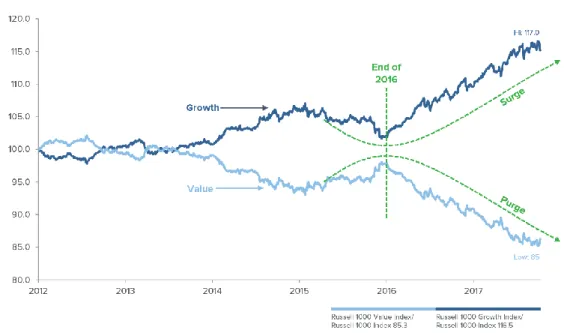
In the last years before the health crisis, value investments had been lower. In some periods, their performance was higher than that of growth investment, which experienced a 264% growth in the Russell 1000 index; the corresponding index of value investments increased by 91%. This situation was likely caused by outperforming technology-related stocks (growth category) and underperforming energy and financials (value category).
The effectiveness of value investing in recent years has been questioned due to fluctuations caused by the COVID-19 pandemic. Companies’ spending habits have undergone significant changes, which may cause a change in their intrinsic value and cause investors to reassess their investments given market reactions to the COVID 19 health crisis (Ashraf, 2020).
During the onset of the pandemic, growth stocks led to lower-value stocks in March 2020, putting the yield gap between the two types of investments at 22.5 points (Bogdanova, 2020).
Fallahgoul (2021) reflected how in early 2021, value stocks increased and growth stocks decreased due to vaccine-related reductions in COVID-19 cases, which caused the start of the economic recovery in the United States.
4
This research investigates stocks’ value and growth behavior by analyzing their trends before and after the COVID-19 health crisis, using unit root techniques and measurement methods. This study uses fractional integration, such as ARFIMA, and applies wavelet analysis to check the correlation between the two investment forms to determine which is more influential. The results show that while growth stocks return to their original state after exogenous shocks, value investments undergo permanent changes in the face of shocks; however, after the COVID-19 crisis, the value of the MSCI reverses in the face of the shock, so it is unnecessary to take additional measures. In contrast, for MSCI growth, policies must be applied so that the shares return to their original trends.
Both types of investments are parallel until 2017, after which growth investment begins to dominate.
Source: Fundstrat, Bloomberg
Figure 1. S&P 500 Growth and Value relative price performance
5
2. Literature Review
The extant literature has thoroughly examined value and growth investing. For example, Sharpe et al. (1993) studied the performance of both types of investment in France, Germany, Switzerland, England, Japan, and the US through the price/earnings ratio, finding that actions by value exceed actions by growth in all markets throughout the period analyzed.
Rosenberg et al. (1985) and Fama and French (1992), among others, indicated that the outperformance of value stocks might be due to time-varying risk; the risk of non-value growth strategies is high in bad times when the premium expected by the risk is high, and it is low in good times when the expected risk premium is low.
Furthermore, Petkova and Zhang (2005) analyzed the risk of value and growth stocks, finding that the variable risk in time can explain the value premium, the value betas tend to covary positively, and growth betas tend to covary negatively with expected market risk. Additionally, Reuer and Tong (2007) stated that the outperformance of value investing is controversial, as some researchers attribute this fact to the higher risk of value stocks, while others argue that the rewards come from the cognitive biases underlying investor behavior (Barberis & Thaler, 2003).
When conditional volatilities are high, the expected excess returns of value stocks are more sensitive to economic conditions than the expected returns of growth stocks. This situation implies that the expected value premium varies over time, shooting up when with high volatility before gradually decreasing (Gulen et al., 2011).
Research by Cronqvist et al. (2015) suggested that investors with adverse macroeconomic experiences can be reluctant to invest in growth, placing great interest in value investments. Sandy Nairn of the Templeton Global Equity Group said that methodological discussions regarding indices are meaningless (Nairn, 2002), along the
6
same lines as the Fama research, 1998. A value stock in the United States could be transformed into a growth stock if it were located in Europe. Both types of investment show a similar performance, which largely depends on macroeconomic factors, showing the most significant differences in shocks, such as the dot-com bubble or the COVID-19 pandemic (Figure 2).
Source: RBC Wealth Management, Bloomberg Figure 2. Russell 1000 Growth and Value Indexes
2.1. Growth Investment
MacLean et al. (2011) define growth stocks as those representing companies that have demonstrated above-average earnings growth in recent years, with the expectation of continuing to deliver high earnings growth values.
7
Beneda (2002) indicated that the long-term performance of growth stocks is higher than that obtained with value stocks for portfolios created between 1990 and 2000; however, after five years, growth stocks were lagging behind the value ones.
Existing studies have examined growth options with different characteristics, such as alliances between companies and joint ventures (Chi, 2000; Kumar, 2005), venture capital investments (Hurry et al., 1992; Li and Chi, 2013), and multinational investments (Kogut, 1983).
Belderbos et al. (2019) analyzed how companies can create value from their investments’
growth options based on a framework that integrates the roles of heterogeneity and uncertainty in the company, being central concepts in strategic management and real options research.
During the health crisis, the growth stock spread reached levels not seen since the dot- com boom of 2000. In March 2020, this success accelerated as the economy suffered from lockdown, prompting investors to turn to known investments (Figure 3). The Russell 1000 growth index soared 81.1% from its low on 22 March to 31 December 2020 due to technology companies, clear beneficiaries of the strong push for digitization during the pandemic.
This trend changed at the end of February 2021 with a decrease of 0.8%; however, it increased in the second quarter of 2021 due to a rise in the bond market, decreasing yields and easing the pressure inflation on growth stocks, topping value 39.7%, according to MSCI.
.
8 Source: MSCI
Figure 3. MSCI Growth Value from January 1997 to June 2021
2.2. Value Investment
Value investing is an investment strategy in which stocks that appear to be trading for less than their book or intrinsic value are selected. Investors seek to invest in what is considered to be undervalued in the market, betting on an overreaction to good and bad news and, consequently, offering the opportunity to generate profits. Graham et al. (1934) presented value investing with the caution of a comprehensive analysis that included qualitative and quantitative discussions.
Lakonishok et al. (1994) stated that value returns are higher than returns to growth in times of economic stability, being lower during recessions, a result that contradicts the risk hypothesis. Chopra et al. (1992) concurred in analyzing the investment effect, an earlier manifestation of the value premium. Both studies agreed that this value does not expose investors to greater risk.
Over the years, despite different economic cycles, value investing has maintained a good record, experiencing vicissitudes in the 20th century (Asness et al., 2015).
Value stocks have lagged behind growth investments in recent years, having brief periods of outperformance in the US; since early 2010, the US Russel 1000 Growth Index has risen 264%, while the increase in the value index has been 91%. This situation is likely
9
due to the significantly outperforming technology-related stocks in the growth category and underperforming energy and financials in the value category (Figure 4).
Value investment metrics are used as benchmark data to make sense of performance value before and after the onset of the pandemic; Zhou and Liu (2021) theoretically assumed that the COVID-19 pandemic created potential, influencing the relevance, accuracy, and validity of value investment indicators.
Source: Bloomberg Intelligence, RBC Wealth Management Figure 4. Global Value Stocks vs. Inflation Expectations
2.3. Value and Growth Investment Analysis Methods
De Jong and Apilado (2009) conducted a study based on the use of Augmented Dickey–
Fuller (ADF) (1981) and the Ng–Perron test for the analysis of the stationarity of the data, demonstrating that the relationship between forecast earnings and actual earnings should converge over the long term in the predictions. The results suggested that earnings forecasts for both stock groups could be biased.
Using the Phillips–Perron (PP) unit root test, Chiang (2016) analyzed the transitional behavior between value and growth stocks, determining that annual stock returns were
10
positively related to contemporary changes in stock prices, earnings per share, and growth rates, managing to describe the behavior between value and growth stocks.
In their study, Saydar and Bedir (2021) demonstrated the existence of a margin between the commercial value and the intrinsic value in value investments regarding the price/book value and price/earnings ratios. To achieve this, they applied the value investment criteria to a selected portfolio to test the validity of the hypothesis. In this way, they help determine the actual value of a stock whose current price is below its real value.
The forecast of share prices has been a fundamental pillar in the stock markets.
Developing different predictive methods with this objective and the rise of neural networks, Tseng et al. (2012) developed neural networks to perform the prediction of daily stock prices.
3. Data and Methodology 3.1. Dataset
To analyze the behavior of the growth and value investment strategy, we use the MSCI International World Index Value Price Index USD Real-time and MSCI International World Index Growth Price Index USD Real-time, respectively, in daily frequency from 23 January 2009 to 3 June 2022. These indices comprise the weighting of investment funds’ stock market indices and portfolio analysis; the time series were obtained from the Thomson Reuters Eikon database.
Figure 4 presents the trend of both indices. Throughout the time series, it is appreciated as the strategy based on value investing has a greater gap than the strategy based on growth investing. Since the beginning of the COVID-19 crisis, the situation has reversed in favor of growth stocks.
11 Figure 5. MSCI value and MSCI Growth
To conduct the analysis considering the COVID-19 health crisis, we divided the data based on the global declaration of a pandemic, using the dates indicated in the following table as a reference.
Dataset classification COVID-19
1st period January 23, 2009 November 15, 2019
2nd period November 18, 2019 June 03, 2022
Table 1. Dataset classification
3.1.1. Unit Roots
The augmented Dickey–Fuller (ADF) test, based on Fuller (1976) and Dickey and Fuller (1979), was used to determine the stationarity of this paper’s data. In addition, this study used a non-parametric estimate of the spectral density of 𝑢𝑡 (the zero frequency) based on Phillips (1987) and Phillips and Perron (1988) and deterministic trend estimates based
12
on Kwiatkowski et al. (1992), Elliott et al. (1996), and Ng and Perron (2001) because they have greater estimation power.
3.1.2. ARFIMA (p, d, q) model
To carry out this research, we also employ fractionally integrated methods to obtain the stationary time series. We achieved this objective, 𝐼(0), by differentiating the time series with a fractional number.
Using a mathematical notation, a time series 𝑥𝑡, 𝑡 = 1, 2, … follows an integrated order process 𝑑, denoted as 𝑥𝑡≈ 𝐼(𝑑)) if:
(1 − 𝐿)𝑑𝑥𝑡= 𝑢𝑡, 𝑡 = 1, 2, …, (1)
where 𝑑 refers to any real value, and 𝐿 indicates the lag operator (𝐿𝑥𝑡 = 𝑥𝑡−1). 𝑢𝑡 is a covariance stationary process I(0) where the behavior of the spectral density function shows in the weak form, a type of time dependence where the function is positive and finite at the zero frequency.
xt is ARFIMA (p, d, q) when is ARMA𝑢𝑡 (p, q). Therefore, depending on the value of parameter 𝑑 on (1), the reading of the results can be as follows. xt is anti-persistent if d <
0 (Dittmann and Granger, 2002); when 𝑑 = 0 in (1), we say that the process is short memory I(0), and with a high degree of association over a long time, we say that the process is long memory (d > 0). d < 1 means that the shock is transitory, and the series revert to the mean; finally, when d ≥ 1, we expect that the shocks are permanent.
We follow the methodology proposed by Sowel (1992) instead of those proposed in other research (Geweke and Porter-Hudak, 1983; Phillips, 1999, 2007; Sowell, 1992a, b;
Robinson, 1994, 1995a, b). The maximum likelihood estimate of 𝑑 (Sowell, 1992a, b) jointly estimates 𝑝, 𝑑, and 𝑞 (the associated standard errors) to determine whether the series is stationary or integrated. Additionally, according to Box-Steffensmeier and
13
Tomlinson (2000), using this methodology, the estimate of d addresses concerns from critics of Box-Jenkins time series analysis and the “art” of interpreting autocorrelation functions (acfs) and partial autocorrelation functions (pacfs) to determine the characterization of the series, eliminating the casual component.
To select the most appropriate ARFIMA model, we use the Akaike information criterion (AIC) (Akaike, 1973) and the Bayesian information criterion (BIC) (Akaike, 1979).
3.1.3. FCVAR model
Johansen (2008) introduced the fractionally cointegrated vector autoregressive (FCVAR) to check a multivariate model from a fractional point of view. Johansen and Nielsen (2010) further expanded this model by being a step ahead of the cointegrated vector autoregressive (CVAR) model proposed by Johansen (1996), allowing the series to be integrated in order d and cointegrated in order d–b, with b > 0. To understand the FCVAR model, first, we introduce the non-fractional CVAR model.
If 𝑌𝑡, 𝑡 = 1, … , 𝑇 is a p-dimensional I(1) time series, and the CVAR model can be represented as follows:
𝛥𝑌𝑡 = 𝛼𝛽′𝑌𝑡−1+ ∑𝑘𝑖=1𝛤𝑖𝛥𝑌𝑡−𝑖+ 𝜀𝑡 = 𝛼𝛽′𝐿𝑌𝑡+ ∑𝑘𝑖=1𝛤𝑖𝛥𝐿𝑖𝑌𝑡+ 𝜀𝑡. (2) The difference and the lag operator are represented by ∆𝑏 and 𝐿𝑏 = 1 − ∆𝑏, which are used to derive the FCVAR model, obtaining
∆𝑏𝑌𝑡 = 𝛼𝛽′𝐿𝑏𝑌𝑡+ ∑𝑘𝑖=1𝛤𝑖𝛥𝐿𝑖𝑏𝑌𝑡+ 𝜀𝑡, (3) which is applied to 𝑌𝑡= ∆𝑑−𝑏𝑋𝑡, such that
∆𝑑𝑋𝑡 = 𝛼𝛽′𝐿𝑏∆𝑑−𝑏𝑋𝑡+ ∑𝑘𝑖=1𝛤𝑖𝛥𝑏𝐿𝑖𝑏𝑌𝑡+ 𝜀𝑡, (4) where 𝜀𝑡 is a mean zero term. 𝛺 is the p-dimensional independent and identical distributed variance-covariance matrix. The 𝛼 and 𝛽 matrices have a form 𝑝 × 𝑟 where 0 ≤ 𝑟 ≤ 𝑝,
14
and 𝛽 allows us to identify the relationship in the long run in terms of cointegration. 𝛤𝑖 is related to the short-run behavior of the variables and their controls. Finally, 𝛼 indicates the deviations from the equilibria and the speed of the adjustment.
The FCVAR model is developed in a computer programming language such as Matlab (Nielsen and Popiel, 2018). This model has been employed in numerous empirical papers (Jones et al., 2014; Baruník and Dvořáková, 2015; Maciel, 2020; Aye et al., 2017;
Dolatabadi et al., 2018; Gil-Alana and Carcel, 2020; Poza and Monge, 2020; Monge and Gil-Alana, 2021).
3.1.4. Wavelet analysis
The wavelet methodology allows time series to be analyzed in the time-frequency domain; thus, this paper uses wavelet coherency and wavelet phase difference1 because the requirement of stationarity is not necessary, and studying the interaction in the time and frequency domain of the time series shows us evidence of potential changes (structural changes).
Based on the analysis by Kyrtsou et al. (2009) regarding the energy markets and nonlinear dependencies, several authors have used nonlinear methods to analyze the impact of oil shocks using wavelet analysis. Other authors, such as Aguiar-Conraria and Soares (2014) and Crowley and Mayes (2009), have used wavelets to test and study business cycle synchronization.
Additionally, the most distinguished information is hidden in the signal’s frequency content; therefore, we can define the time series as an aggregation of components operating on different frequencies. Finally, if we follow Zhou (2008), Podobnik and
1Continuous wavelet transform (CWT) has been applied in several finance and economics studies, such as Vacha and Barunik (2012), Aguiar-Conraria and Soares (2011, 2014), Dewandaru et al. (2016), Tiwari et al. (2016), and Jammazi et al. (2017), among others.
15
Stanley (2008), Gu and Zhou (2010), and Jiang and Zhou (2011), we can conclude that if we apply a cross-correlation to study the statistical relationships between two multifractal time series, our results might be misleading.
The wavelet coherency plot represents the correlation of time series and helps us to identify hidden patterns and information in the time-frequency domain. The wavelet transform, represented by 𝑊𝑇𝑥(𝑎, 𝜏) of a time series 𝑥(𝑡), is obtained by projecting a mother wavelet ψ, is defined as
𝑊𝑇𝑥(𝑎, 𝜏) = ∫ 𝑥(𝑡) 1
√𝑎𝜓∗(𝑡−𝜏
𝑎 ) 𝑑𝑡
+∞
−∞ , (5)
where the wavelet coefficients of 𝑥(𝑡) are represented by 𝑊𝑇𝑥(𝑎, 𝜏) and provide information on time and frequency by mapping the original time series onto a function of 𝜏 and 𝑎. Following Aguiar-Conraria and Soares (2014), we choose the Morlet wavelet as
the mother wavelet because it is a complex sine wave within a Gaussian envelope; thus, we can measure the synchronism between time series.
Wavelet coherence helps us understand how one time series interacts with the other. We can define this term as
1. 𝑊𝐶𝑂𝑥𝑦= 𝑆𝑂(𝑊𝑇𝑥(𝑎,𝜏)𝑊𝑇𝑦(𝑎,𝜏)∗)
√𝑆𝑂(|𝑊𝑇𝑥(𝑎,𝜏)|2)𝑆𝑂(|𝑊𝑇𝑦(𝑎,𝜏)|2)
, (6)
where the smoothing operator in time and scale is represented with the parameter SO.
This operator is essential because, without it, the wavelet coherency is always one for all times and scales (see Aguiar-Conraria et al., 2008, for details). The Matlab codes for the CWT resolution are available on Aguiar-Conraria’s website.2
3.1.5. Machine learning
The groupings of neurons in different layers characterize neural networks (Zhang et al.,
2 https://sites.google.com/site/aguiarconraria/joanasoares-wavelets
16
2020). A neural network contains three layers. The input layer is responsible for receiving data to be analyzed and sending it to the subsequent layers, the intermediate layers or hidden layers are where the nonlinear processing of the data is performed, and the output layer provides a result for each of the inputs (Rumelhart et al., 1986).
No applicable methodology exists for choosing the number of layers, and the most used is the trial-and-error approach proposed by Güler and Übeyli (2005).
The architecture of a neural network is defined by the following formula:
𝐼 − (𝐻1, 𝐻2, 𝐻3, … , 𝐻𝑁) − 𝑂 (7)
where I represents the number of neurons in the input layer. Hn indicates the nodes that make up the hidden layer n, and O is the number of neurons in the output layer.
Neurons in one layer are connected to each neuron in the next layer (Fu, 1994), and each of these connections is assigned a weight calculated based on the neural network results compared to the expected result. This error is sent to the previous layers, allowing the calculation of the adjusted weights throughout the training. In this process, the data must be divided into two groups; the first group trains the neural network, and the second evaluates the model’s accuracy. The mean square error (MSE) is the most widely used error metric, and the main objective is to achieve the lowest possible value.
In Figure 6, Yj represents the input vector, which expands as 𝑌𝑗 = {𝑦1, 𝑦2, 𝑦3, … , 𝑦𝑛}; the vector of weights between the j nodes of the first layer to the k nodes of the first hidden layer is represented as 𝑊𝑗𝑘(𝑗 = 1, 2, 3, … , 𝑛; 𝑘 = 1, 2, 3, … , 𝑚). The vector relative to the k neurons in the hidden layers is represented by 𝑋𝑘(𝑘 = 1, 2, 3, … , 𝑚), which is
determined by the following formula 𝑋𝑘= 𝑓(∑𝑛𝑗=1𝑊𝑗𝑘𝑌𝑗+Θ𝑘). 𝑊𝑘(𝑘 = 1, 2, 3, … , 𝑚) reflects the weights on the connections of the nodes from the last hidden layer to the output layer, and the resulting vector of the output layer of the neural network with one neuron is Y, determined by 𝑌 = 𝑓(∑𝑛𝑘=1𝑊𝑘𝑋𝑘+Θ). Finally, Θ represents the
17
polarization value of the last layer, while the polarization value of the hidden layer nodes is defined by Θ𝑘(𝑘 = 1, 2, 3, … , 𝑘).
Figure 6. Artificial Neural Network for
time series forecasting.
Arbib (1995), Simpson and Brotherton (1995), and Arbib et al. (1997) state that it is possible to make predictions in different areas of knowledge, such as medicine and economics, using neural networks, which produce better results than traditional statistical models (de Lillo and Meraviglia, 1998; Arana et al., 2003). Neural networks can learn relationships between the different variables that make up the data set thanks to parallel processing.
Various studies, such as Hinton and Salakhutdinov (2006), initiated the development of deep learning by demonstrating the ability to train neural networks through the correct initialization of weights and a large number of deep layers instead of setting random values. In this process, each layer is initially trained unsupervised, and supervised training is later conducted, establishing the resulting weights of the previously trained layers as initial values.
An efficient weight initialization scheme proposed by Glorot and Bengio (2010), commonly known as Xavier initialization, provides the ability to initialize the weights without needing supervised training. This methodology has become the standard for deep
18
learning, demonstrating a significant impact on training performance and increased accuracy thanks to the choice of a nonlinear activation function. This approach has given rise to research to evaluate the different activation functions and the existing ones to locate the most suitable function to identify the rectified linear unit (Jarrett et al., 2009;
Nair and Hinton, 2010; Glorot et al., 2011).
The data obtained in Section 3 is next divided into two sets: training with 80% of the data and validation with the remaining 20%. The test group was established for model validation by checking the MSE. The division is made based on Gholamy et al. (2018), which indicated an improvement in the results by performing an 80–20 division, thus avoiding the overfitting of the neural network. The model evaluation is performed using the MSE and root mean square error metrics.
4. Empirical Results
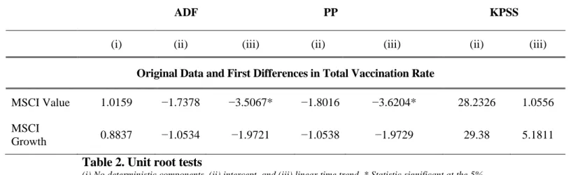
We calculated the three standard unit root tests to analyze the stationarity between investment strategies based on value and growth.
Table 2 displays the results using these methodologies, showing that in both time series, the data have a stationary I(1) behavior except in the cases of linear time trend (iii) in MSCI Value.
19
ADF PP KPSS
(i) (ii) (iii) (ii) (iii) (ii) (iii)
Original Data and First Differences in Total Vaccination Rate
MSCI Value 1.0159 −1.7378 −3.5067* −1.8016 −3.6204* 28.2326 1.0556 MSCI
Growth 0.8837 −1.0534 −1.9721 −1.0538 −1.9729 29.38 5.1811
Table 2. Unit root tests
(i) No deterministic components, (ii) intercept, and (iii) linear time trend. * Statistic significant at the 5%
level.
Using unit root methods in the time series, we verified that the data are nonstationary I(1) and concluded that we must use the first differences. Conversely, we use fractional alternatives, such as ARFIMA (p, d, and q) models, due to the low power of the unit root methods3 to study the persistence of the time series related to commodity spot prices.
The exact maximum likelihood estimation approach to estimate the ARFIMA (𝑝, 𝑑, 𝑞) model based on Sowell (1992a, b) requires the specification of the 𝑝 and 𝑞 values and the full ARFIMA model conditional on these choices. This approach involves choosing appropriate autoregressive (AR) and moving average (MA) specifications.
The AR part is based on the idea that the current value of the series can be explained as a linear combination of p past values, with a random error in the same series. In contrast, the MA part states that the following observation is the mean of every past observation.
We considered 𝑝, 𝑞 ≤ 2 for several reasons. First, the literature related to ARFIMA models uses a value up to 2 in the autoregressive and MA part. Second, the more the lags and MAs are considered, the more abstract the model becomes, and the more observations are lost. Finally, we apply the principle of parsimony, where the more straightforward theory (model) has the greatest probability of being correct.
3 See Diebold and Rudebusch (1991), Hassler and Wolters (1994), and Lee and Schmidt (1996).
20
To construct the ARFIMA model to obtain the appropriate AR and MA orders, we consider the AIC (Akaike, 1973) and the BIC (Akaike, 1979).4
For each time series, Table 3 presents the fractional parameter 𝑑 and the AR and MA orders obtained using Sowell’s (1992a, b) maximum likelihood estimator, considering 𝑝, 𝑞 ≤ 2.
Table 3. Results of long-memory tests
4 A point of caution should be adopted here since the AIC and BIC may not be the best criteria for applications involving fractional models (Hosking, 1981).
Long-Memory Test
Data Analyzed
Sample Size (Days)
Model Selected d Std. Error Interval I(d) MSCI Value 3484 ARFIMA (0, d, 1) 1.02 0.022 [0.99, 1.06] I(1) MSCI Growth 3484 ARFIMA (2, d, 1) 0.97 0.029 [0.93, 1.02] I(1)
Before COVID-19
MSCI Value 2819 ARFIMA (0, d, 0) 1.07 0.017 [1.04, 1.10] I(1)
MSCI Growth 2819 ARFIMA (0, d, 0) 1.06 0.017 [1.04, 1.09] I(1) After COVID-19
MSCI Value 665 ARFIMA (2, d, 1) 0.98 0.080 [0.85, 1.11] I(1)
MSCI Growth 665 ARFIMA (2, d, 1) 1.00 0.065 [0.89, 1.11] I(1)
21
Focusing on the original time series in Table 2, we observe that the value of 𝑑 is below 1 for MSCI Growth; therefore, we support the mean reversion that implies transitory shocks. Thus, in the event of exogenous shocks, the series returns to its original trend in the future; in this case, Hypothesis I(1) cannot be rejected. Conversely, we observe a different behavior and higher level of persistence in the MSCI Value where 𝑑 = 1.02.
This result provides is no evidence of mean reversion, and the shocks are expected to be permanent (e.g., lasting forever), causing a change in trend.
Focusing on the behavior after COVID-19, we observe that the fractional parameter for the MSCI value is lower than 1 (𝑑 = 0.98) that means mean reversion. This result indicates that additional measures are unnecessary since the series return to their long- term projections; however, according to the confidence interval, we cannot reject Hypothesis I(1), where the shock effect persists indefinitely, due to the confidence intervals being very wide.
Finally, for MSCI Growth after Covid-19, we conclude that the authorities require strong measures to recover the original trend when shock occurs.
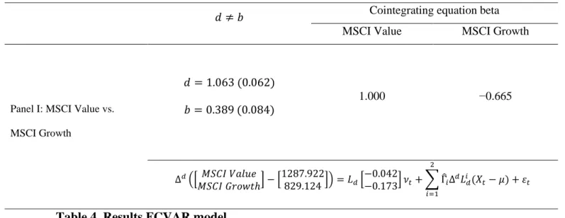
To analyze the long-run co-movements of both time series, we perform the FCVAR model proposed by Johansen and Nielsen (2012). Table 4 summarizes the results.
22
Table 4. Results FCVAR model
Panel I in Table 4 indicates that the order of integration for the individual series is about 1.063. In contrast, the reduction in the degree of integration in the cointegrating regression is 0.389, implying an order of integration of about 0.674 for the cointegrating relationship.
We conclude that the resulting long-run equilibrium time series follows a long-memory process, which suggests potential forecasting power at longer horizons (Baillie and Bollerslev, 1994). Furthermore, this value (𝑑 − 𝑏 = 0.674) implies that the duration of the shock is long-lived (although it is mean-reverting), and the error correction term follows a nonstationary process.
Additionally, we used a multivariate wavelet analysis on the time-frequency domain to analyze the correlation between the two forms of investment and which is more influential.
𝑑 ≠ 𝑏 Cointegrating equation beta
MSCI Value MSCI Growth
Panel I: MSCI Value vs.
MSCI Growth
𝑑 = 1.063 (0.062) 𝑏 = 0.389 (0.084)
1.000 −0.665
∆𝑑([𝑀𝑆𝐶𝐼 𝑉𝑎𝑙𝑢𝑒
𝑀𝑆𝐶𝐼 𝐺𝑟𝑜𝑤𝑡ℎ] − [1287.922
829.124]) = 𝐿𝑑[−0.042
−0.173] 𝜈𝑡+ ∑ Γ̂𝑖Δ𝑑𝐿𝑖𝑑(𝑋𝑡− 𝜇
2
𝑖=1
) + 𝜀𝑡
23 Figure 7. Wavelet Coherency and Phase-differences
Figure 7 shows when and at which frequencies the interrelations between the time series occur and when they are the strongest. Section (a) of the figure indicates the wavelet coherency identifying the main regions with statistically significant coherency.
We can observe two distinct parts in the wavelet coherence analysis. The first is between 2000 and the end of 2016; the second is between 2018 and mid-2020, with a high correlation between the highest (short-term) and lowest frequencies (long term). The frequencies range from 0.5 to 128.
To obtain information about the relationship between both time series, we examine the results obtained in sections (b) and (c) of the figure, the partial phase difference, and the partial wavelet gain, respectively. In the short-term (1–12 frequency band), the phase difference is between 0 and −𝜋/2 throughout the analyzed period, indicating that a growth-based investment strategy is more successful than a value-based investment strategy.
If we focus on the medium-long term, we observe that the behavior of both investment strategies is in line until 2017, when an investment strategy based on growth predominates again.
24
To provide further precision to this research, we used artificial intelligence to predict a neural network model, corroborate the results obtained by traditional statistical techniques, and analyze the behavior of the stock-by-value and stock-by-growth indices.
To make the prediction using an artificial neural network (ANN) model, a novel hybrid model combines bidirectional long short-term memory type networks and a graph convolutional network model, whose results demonstrate greater precision in the prediction of neural networks compared to traditional statistical techniques and other ANN models.
Following Mapuwei et al. (2020), the MSE and RMSE metrics are used to evaluate the model, being the most used in prediction methods with machine learning techniques (Barrow and Crone, 2016b). The MSE is the most used cost function in regression problems, calculating the squared difference between the predicted value y’ and the actual value y.
l(i)(w,b) = (y’(i) − y(i))2 (8)
The following table shows the results of the precision obtained by the ANN model, using the data related to January 2021 as a reference; the results obtained are in line with the literature, with results very close to zero, being the model with less error to make predictions of time series.
MSCI International World Index Growth Price Index USD Real-time
MSCI International World Index Value Price Index USD Real-time
MSCI (1 January 2021) 4795.04 USD 3305.71 USD
Results obtained in our forecast 4794.49 USD 3305.22 USD
MSE of the ANN model 0.011 0.01
Deviation from MSCI price 0.54 0.45
Table 4. Forecast results and accuracies of the time series of MSCI
25
The results indicate that de ANN has an MSE of 0.01, and a deviation from de MSCI is 0.54 and 0.45.
Figure 8 shows how after the shock due to the COVID-19 pandemic, both the values of investments by value and growth show upward trends, being more pronounced in growth stocks; this finding coincides with the results obtained.
Predictions made with neural networks show an increase in both types of investments in the second half of 2022 and an increase of 42% for growth stocks and 22% for value stocks compared to the same pre-pandemic dates in 2019.
Figure 8. Forecasting of MSCI value and MSCI Growth
5. Conclusions
Research on strategic management and real options requires a balance between the expectations of high earnings growth values and the roles of heterogeneity and
26
uncertainty in organizations. Forecasting stock prices is then required, which is possible through the development of reliable predictive methods and accurate analytics on the performance of value and growth stocks in changing scenarios, reflecting the virtue of prudence.
The importance of this research lies in using that prudence when investing in deep knowledge of investments by value and growth. Therefore, this paper’s primary objective is to examine the behavior and trend of stocks by value and growth before and after the crisis caused by SARS-COV 2, which caused a significant shock in investor behavior, given the situation resulting from the economic paralysis.
The analysis includes data from Thomson Eikon Reuters, corresponding to the MSCI International World Index Value Price Index USD Real-time and MSCI International World Index Growth Price Index USD Real-time. For statistics of both types of investments, unit root techniques are carried out, including ADF (Dickey and Fuller, 1979), PP (Phillips and Perron, 1988), and KPSS (Kwiatkowski et al., 1992), to check the stationarity of the series as well as its behavior; the results show that the first difference should be used after verifying that it is a stationary series. Subsequently, fractional integration techniques are applied to measure the degree of persistence in the face of economic shocks that may occur. A wavelet analysis can then determine the correlation between both forms of investment and which one exerts greater influence.
The results from analyzing the period after COVID-19 show that the trend of the growth- based investment strategy has changed, implying permanent effects of the shock, while the value-based investment strategy returns to its long-term trend. We confirm these results by analyzing the long-term behavior of both variables using fractional cointegration and a wavelet-based correlation analysis.
27
ANNs are applied to forecast stock value and confirm the performance of the MSCI value and MSCI growth. The prediction shows how the two indices recovered and exceeded the trend before the health crisis and that this will continue in the second half of 2022; these results align with the existing literature (Liao et al., 2022).
Therefore, we conclude that the pandemic has brought a new scenario where growth stocks prevail over value stocks in the short and medium terms, possibly because growth stocks tend to perform better in changing markets and uncertain scenarios. Still, it is unclear why this did not happen in previous economic crises. Perhaps it can be explained by the fact that the COVID-19 pandemic was an economic crisis, and economic uncertainty was combined with health (contagions and deaths) and social elements (confinement and changes in coexistence patterns), making the scenario much more difficult to read than previous crises, increasing the feeling of illegibility and modifying the decision-making logic.
28
References
Aguiar-Conraria, L., Azevedo, N., & Soares, M. J. (2008). Using wavelets to decompose the time–frequency effects of monetary policy. Physica A: Statistical mechanics and its Applications, 387(12), 2863-2878.
Aguiar-Conraria, L. and Soares, M. J. (2011). Oil and the macroeconomy: Using wavelets to analyze old issues. Empirical Economics, 40(3), 645-655.
Aguiar‐Conraria, L. and Soares, M. J. (2014). The continuous wavelet transform: Moving beyond uni‐ and bivariate analysis. Journal of Economic Surveys, 28(2), 344-375.
Akaike, H. (1973). Maximum likelihood identification of Gaussian autoregressive moving average models. Biometrika, 60(2), 255-265.
Akaike, H. (1979). A Bayesian extension of the minimum AIC procedure of autoregressive model fitting. Biometrika, 66(2), 237-242.
Akinde, M. A., Peter, E. and Ikpefan, O. A. (2019). Growth versus value investing: A case of Nigerian Stock Market. Investment Management and Financial Innovations, 16(1), 30-45.
Alda, M. (2021). The environmental, social and governance (ESG) dimension of firms in which social responsible investment (SRI) and convention pension funds invest:
The mainstream SRI and the ESG inclusion. Journal of Cleaner Production, 298.
Aristotle (1999). Nicomachean ethics. Translated by T. Irwin and Hacket Publishing Company.
Arana, E., Martí-Bonmatí, L., Bautista, D. and Paredes, R. (2003). Diagnóstico de las lesiones de la calota. Selección de variables por redes neuronales y regresión logística. Neurocirugía, 14(5), 377-384.
Arbib, M. A. (1995). Brain theory and neural networks. Cambridge, MA: MIT Press.
Arbib, M. A., Érdi, P. and Szentágothai, J. (1997). Neural organization. MIT Press.
Ashraf, B. N. (2020). Stock markets’ reaction to COVID-19: Cases or fatalities?.
Research in international business and finance, 54, 101249.
Asness, C., Frazzini, A., Israel, R. and Moskowitz, T. (2015). Fact, fiction, and value investing. The Journal of Portfolio Management, 42(1), 34-52.
Aye, G. C., Carcel, H., Gil-Alana, L. A. and Gupta, R. (2017). Does gold act as a hedge against inflation in the UK? Evidence from a fractional cointegration approach over 1257 to 2016. Resources Policy, 54, 53-57.
Baillie, R. T. and Bollerslev, T. (1994). Cointegration, fractional cointegration, and exchange rate dynamics. The Journal of Finance, 49(2), 737-745.
29
Barberis, N., & Thaler, R. (2003). A survey of behavioral finance. Handbook of the Economics of Finance, 1, 1053-1128.
Barrow, D. K., & Crone, S. F. (2016). Cross-validation aggregation for combining autoregressive neural network forecasts. International Journal of Forecasting, 32(4), 1120-1137.
Baruník, J. and Dvořáková, S. (2015). An empirical model of fractionally cointegrated daily high and low stock market prices. Economic Modelling, 45, 193-206.
Belderbos, R., Tong, T. W. and Wu, S. (2019). Multinational investment and the value of growth options: Alignment of incremental strategy to environmental uncertainty.
Strategic Management Journal, 40(1), 127-152.
Beneda, N. (2002). Growth stocks outperform value stocks over the long term. Journal of Asset Management, 3(2), 112-123.
Bogdanova, K. (2020). Growth versus value investing in a COVID-19 world. Source.
Available online: https://www.rbcwealthmanagement.com/en- ca/insights/growth-versus-value-investing-in-a-covid-19-world (Accessed on 22 June 2022).
Box-Steffensmeier, J. M. and Tomlinson, A. R. (2000). Fractional integration methods in political science. Electoral Studies, 19(1), 63-76.
Chahine, S. (2008). Value versus growth stocks and earnings growth in style investing strategies in Euro-markets. Journal of Asset Management, 9(5), 347-358.
Chan, L. K. C. and Lakonishok, J. (2004). Value and growth investing: Review and update. Financial Analysts Journal, 60(1), 71-86, DOI: 10.2469/faj.v60.n1.2593.
Chi, T. (2000). Option to acquire or divest a joint venture. Strategic Management Journal, 21(6), 665-687.
Chiang, G. (2016). Exploring the transitional behavior among value and growth stocks.
Review of Quantitative Finance and Accounting, 47(3), 543-563.
Chopra, N., Lakonishok, J. and Ritter, J. R. (1992). Measuring abnormal performance?
Journal of Financial Economics, 31(2), 235-268.
Cronqvist, H., Siegel, S. and Yu, F. (2015). Value versus growth investing: Why do different investors have different styles? Journal of Financial Economics, 117(2), 333-349.
Crowley, P. M. and Mayes, D. G. (2009). How fused is the euro area core?: An evaluation of growth cycle co-movement and synchronization using wavelet analysis. OECD Journal: Journal of Business Cycle Measurement and Analysis, 2008(1), 63-95.
30
De Jong, P. J. and Apilado, V. P. (2009). The changing relationship between earnings expectations and earnings for value and growth stocks during Reg FD. Journal of Banking and Finance, 33(2), 435-442.
De Lillo, A. and Meraviglia, C. (1998). The role of social determinants on men’s and women’s mobility in Italy. A comparison of discriminant analysis and artificial neural networks. Substance Use and Misuse, 33(3), 751-764.
Dewandaru, G., Masih, R. and Masih, A. M. M. (2016). What can wavelets unveil about the vulnerabilities of monetary integration? A tale of Eurozone stock markets.
Economic Modelling, 52, 981-996.
Dickey, D. A. and Fuller, W. A. (1979). Distribution of the estimators for autoregressive time series with a unit root. Journal of the American Statistical Association, 74(366), 427-481.
Diebold, F. X. and Rudebusch, G. D. (1991). Forecasting output with the composite leading index: A real-time analysis. Journal of the American Statistical Association, 86(415), 603-610.
Dittmann, I. and Granger, C. W. J. (2002). Properties of nonlinear transformations of fractionally integrated processes. Journal of Econometrics, 110(2), 113-133.
Dolatabadi, S., Narayan, P. K., Nielsen, M. Ø. and Xu, K. (2018) Economic significance of commodity return forecasts from the fractionally cointegrated VAR model.
Journal of Futures Markets, 38(2), 219-242.
Elliott, G., Rothenberg, T. J. and Stock, J. H. (1996). Efficient tests for an autoregressive unit root. Econometrica, 64(4), 813-836.
Fallahgoul, H. (2021). Inside the mind of investors during the COVID-19 pandemic:
Evidence from the StockTwits data. The Journal of Financial Data Science, 3(2), 134-148.
Fama, E. F. (1998). Market efficiency, long-term returns, and behavioral finance. Journal of financial economics, 49(3), 283-306.
Fama, E. F. and French, K. R. (1992). The cross-section of expected stock returns. Journal of Finance, 47(2), 427-465.
Fernández, J. L. (2008). Finanzas y ética: La dimensión moral de la actividad financiera y del gobierno corporativa. Madrid: ICADE.
Fu, L. M. (1994). Neural networks in computer intelligence. New York: McGraw-Hill.
Fuller, W. A. (1976). Introduction To Statistical Time Series, New York: JohnWiley.
Geweke, J. and Porter-Hudak, S. (1983). The estimation and application of long memory time series models. Journal of Time Series Analysis, 4(4), 221-238.
31
Gholamy et al. (2018) Gholamy, A., Kreinovich, V. and Kosheleva, O. (2018). Why 70/30 or 80/20 relation between training and testing sets: A pedagogical explanation. Available online: https://scholarworks.utep.edu/cs_techrep/1209/
(Accessed on 22 June 2022).
Gil-Alana, L. A. and Carcel, H. (2020). A fractional cointegration var analysis of exchange rate dynamics. The North American Journal of Economics and Finance, 51.
Glorot, X. and Bengio, Y. (2010, March). Understanding the difficulty of training deep feedforward neural networks. In Proceedings of the thirteenth international conference on artificial intelligence and statistics. JMLR Workshop and Conference proceedings (pp. 249-256).
Glorot, X., Bordes, A. and Bengio, Y. (2011, January). Domain adaptation for large-scale sentiment classification: A deep learning approach. In ICML.
Graham, B., Dodd, D. L. F. and Cottle, S. (1934). Security analysis. New York: McGraw- Hill.
Gu, G. F. and Zhou, W. X. (2010). Detrending moving average algorithm for multifractals. Physical Review. E, 82(1), 011136.
Gulen, H., Xing, Y. and Zhang, L. (2011). Value versus growth: Time‐varying expected stock returns. Financial Management, 40(2), 381-407.
Güler, I. and Übeyli, E. D. (2005). Adaptive neuro-fuzzy inference system for classification of EEG signals using wavelet coefficients. Journal of Neuroscience Methods, 148(2), 113-121.
Hassler, U. and Wolters, J. (1994). On the power of unit root tests against fractional alternatives. Economics Letters, 45(1), 1-5.
Hinton, G. E. and Salakhutdinov, R. R. (2006). Reducing the dimensionality of data with neural networks. Science, 313(5786), 504-507.
Hosking, J. R. M. (1981). Equivalent forms of the multivariate portmanteau statistic.
Journal of the Royal Statistical Society: Series B, 43(2), 261-262.
Hurry, D., Miller, A. T. and Bowman, E. H. (1992). Calls on high-technology: Japanese exploration of venture capital investments in the United States. Strategic Management Journal, 13(2), 85-101.
Jammazi, R., Ferrer, R., Jareño, F. and Shahzad, S. J. H. (2017). Time-varying causality between crude oil and stock markets: What can we learn from a multiscale perspective? International Review of Economics and Finance, 49, 453-483.
Jarrett, K., Kavukcuoglu, K., Ranzato, M. A. and LeCun, Y. (2009, September). What is the best multi-stage architecture for object recognition? In 12th international conference on computer vision 2009 (pp. 2146-2153). IEEE. IEEE.
32
Jiang, Z. Q. and Zhou, W. X. (2011). Multifractal detrending moving-average cross- correlation analysis. Physical Review E, 84(1), 016106.
Johansen, S. (1996). Likelihood-based inference in cointegrated vector autoregressive models. New York: Oxford University Press.
Johansen, S. (2008). A representation theory for a class of vector autoregressive models for fractional processes. Econometric Theory, 24(3), 651-676.
Johansen, S. and Nielsen, M. Ø. (2010). Likelihood inference for a nonstationary fractional autoregressive model. Journal of Econometrics, 158(1), 51-66.
Johansen, S. and Nielsen, M. Ø. (2012). Likelihood inference for a fractionally cointegrated vector autoregressive model. Econometrica, 80(6), 2667-2732.
Jones, M. E. C., Nielsen, M. Ø. and Popiel, M. K. (2014). A fractionally cointegrated VAR analysis of economic voting and political support. Canadian Journal of Economics/Revue Canadienne d’Économique, 47(4), 1078-1130.
Kyrtsou, C., Malliaris, A. G. and Serletis, A. (2009). Energy sector pricing: On the role of neglected nonlinearity. Energy Economics, 31(3), 492-502.
Kogut, B. (1983). Foreign direct investment as a sequential process. In Eds. C.P.
Kindleberger and D.B. Audretsch The Multinational Corporation in the 1980s (pp.
38-56). Boston, MA: MIT Press.
Shyam Kumar, M. V. S. (2005). The value from acquiring and divesting a joint venture:
A real options approach. Strategic Management Journal, 26(4), 321-331.
Kwiatkowski, D., Phillips, P. C. B., Schmidt, P. and Shin, Y. (1992). Testing the null hypothesis of stationarity against the alternative of a unit root. Journal of Econometrics, 54(1-3), 159-178.
Lakonishok, J., Shleifer, A. and Vishny, R. W. (1994). Contrarian investment, extrapolation, and risk. The Journal of Finance, 49(5), 1541-1578.
Lee, D. and Schmidt, P. (1996). On the power of the KPSS test of stationarity against fractionally integrated alternatives. Journal of Econometrics, 73(1), 285-302.
Lewis, A. and Cullis, J. (1990). Ethical investments: Preferences and morality. Journal of Behavioral Economics, 19(4), 395-411.
Li, Y. and Chi, T. (2013). Venture capitalists’ decision to withdraw: The role of portfolio configuration from a real options lens. Strategic Management Journal, 34(11), 1351-1366.
Liao, M. H., Chen, Y. J., Yu, C. W. and Chan, Y. L. (2022). Comparing investor sentiment between growth and value stocks. In International Conference on Innovative
33
Mobile and Internet Services in Ubiquitous Computing (pp. 360-365). Cham:
Springer.
Maciel, L. (2020). Technical analysis based on high and low stock prices forecasts:
Evidence for Brazil using a fractionally cointegrated VAR model. Empirical Economics, 58(4), 1513-1540.
MacLean, L. C., Thorp, E. O. and Ziemba, W. T. (2011). The Kelly capital growth investment criterion: Theory and practice 3. World Scientific.
Mackenzie, C. and Lewis, A. (1999). Morals and markets: The case of ethical investing.
Business Ethics Quarterly, 9(3), 439-452.
Mapuwei, T. W., Bodhlyera, O. and Mwambi, H. (2020). Univariate time series analysis of short-term forecasting horizons using artificial neural networks: The case of public ambulance emergency preparedness. Journal of Applied Mathematics, 2020, 1-11.
Monge, M. and Gil-Alana, L. A. (2021). Lithium industry and the U.S. crude oil prices.
A fractional cointegration VAR and a Continuous Wavelet Transform analysis. Resources Policy, 72, 102040.
Nair, V. and Hinton, G. E. (2010). Rectified linear units improve restricted Boltzmann machines. In Icml.
Nairn, A. (2002). Engines That Move Markets: Technology investing from railroads to the internet and beyond. John Wiley & Sons.
Ng, S. and Perron, P. (2001). Lag length selection and the construction of unit root tests with good size and power. Econometrica, 69(6), 1519-1554.
Nielsen, M. Ø. and Popiel, M. K. (2018). A MATLAB program and user’s guide for the fractionally cointegrated VAR model (Queen’s Economics Department Working Paper no 1330). Ontario, Canada, K7L 3N6.
Petkova, R. and Zhang, L. (2005). Is value riskier than growth? Journal of Financial Economics, 78(1), 187-202.
Phillips, P. C. B. (1987). Time series regression with a unit root. Econometrica, 55(2), 277-301.
Phillips, P. C. B. (1999). Discrete Fourier transforms of fractional processes. Department of Economics, University of Auckland.
Phillips, P. C. B. (2007). Unit root log periodogram regression. Journal of Econometrics, 138(1), 104-124.
Phillips, P. C. B. and Perron, P. (1988). Testing for a unit root in time series regression.
Biometrika, 75(2), 335-346.
34
Podobnik, B. and Stanley, H. E. (2008). Detrended cross-correlation analysis: A new method for analyzing two nonstationary time series. Physical Review Letters, 100(8), 084102.
Poza, C. and Monge, M. (2020). A real time leading economic indicator based on text mining for the Spanish economy. Fractional cointegration VAR and continuous wavelet transform analysis. International Economics, 163, 163-175.
Reuer, J. J. and Tong, T. W. (2007). Corporate investments and growth options.
Managerial and Decision Economics, 28(8), 863-877.
Revelli, C. (2017). Socially responsible investing (SRI): From mainstream to margin?.
Research in International Business and Finance, 39, 711-717.
Robinson, P. M. (1994). Efficient tests of nonstationary hypotheses. Journal of the American Statistical Association, 89(428), 1420-1437.
Robinson, P. M. (1995a). Gaussian semiparametric estimation of long range dependence.
Annals of Statistics, 23, 1630-1661.
Robinson, P. M. (1995b). Log-periodogram regression of time series with long range dependence. Annals of Statistics, 23(3), 1048-1072.
Rosenberg, B., Reid, K. and Lanstein, R. (1985). Persuasive evidence of market inefficiency. Journal of Portfolio Management, 11(3), 9-16.
Rossi, M., Festa, G., Chouaibi, S., Fait, M. and Papa, A. (2021). The effects of business ethics and corporate social responsibility on intellectual capital voluntary disclosure. Journal of Intellectual Capital, 22(7), 1-23.
Rumelhart, D. E., Hinton, G. E. and Williams, R. J. (1986). Learning representations by back-propagating errors. Nature, 323(6088), 533-536.
Saydar, O. O. and Bedir, C. (2021). Value investing analysis of banking sector on BIST- 100. Journal of Economics Finance and Accounting, 8(2), 90-101.
Sciarelli, M., Cosimato, S., Landi, G. and Iandolo, F. (2021). Socially responsible investment strategies for the transition towards sustainable development: The importance of integrating and communicating ESG. TQM Journal, 33(7), 39-56.
Sharpe, W. F., Capaul, C., Rowley, I. and Sharpe, W. F. (1993). International value and growth stock returns. Financial Analysts Journal, 49(1), 27-36.
Simpson, P. K. and Brotherton, T. M. (1995, June). Fuzzy neural network machine prognosis. In Applications of Fuzzy Logic Technology II, 2493. International Society for Optics and Photonics.
Sowell, F. (1992a). Maximum likelihood estimation of stationary univariate fractionally integrated time series models. Journal of Econometrics, 53(1-3), 165-188.
35
Sowell, F. (1992b). Modeling long-run behavior with the fractional Arima model. Journal of Monetary Economics, 29(2), 277-302.
Tiwari, A. K., Mutascu, M. I. and Albulescu, C. T. (2016). Continuous wavelet transform and rolling correlation of European stock markets. International Review of Economics and Finance, 42, 237-256.
Tseng, K. C., Kwon, O. and Tjing, L. C. (2012). Time series and neural network forecasts of daily stock prices. Investment Management and Financial Innovations, 9(1), 32-54.
Vacha, L. and Barunik, J. (2012). Co-movement of energy commodities revisited:
Evidence from wavelet coherence analysis. Energy Economics, 34(1), 241-247.
Zhang, A., Lipton, Z. C., Li, M. and Smola, A. J. (2020). Dive into deep learning 996.
Zhou, W. X. (2008). Multifractal detrended cross-correlation analysis for two nonstationary signals. Physical Review E, 77(6), 066211.
Zhou, Q. and Liu, Y. (2021, June). The effectiveness of the value investment theory during the COVID-19 pandemic: Using the heavy asset industry as an example.
In. Advances in Economics, Business and Management Research International Conference on Enterprise Management and Economic Development (ICEMED 2021). Atlantis Press, 2021, (211-220).