Indications of new physics in the cosmic neutrino spectrum

Indications of new physics in the cosmic neutrino spectrum

−J. M. Carmona

−J. J. Relancio

−J. L. Cortés

−Maykoll A. Reyes TAE. September 19, 2019

Indications of new physics

Indications of new physics

Indications of new physics

Figure 2: IceCube events (log-scale)

Indications of new physics

Figure 3: IceCube events (log-scale)

Indications of new physics

We expect neutrinosin that range due to. . .

• . . .extrapolationof the espectrum at lower energies: Φ∼E_d⁻².

• . . . we should see effects of theGlashow resonance

atE∼6.5 PeV. ^{Figure 4:} IceCube events (log-scale) and interpretation of the flux

Indications of new physics

It has been proposed, among other possibilites, that the cut-off is produced byintrinsic propagation effects.

This kinds of effects exist by the own nature of the neutrino and cause energy loss along the trayectory. If the influence of the effects are strong enough, this might explain the origin of the cut-off.

One intrinsic effect along the propagation is theuniverse

expansion. However, this is not enough to explain the cut-off, so we need to look for effects ofnew physics. For that, we use the Lorentz Invariance Violation.

Indications of new physics

The effects of theLorentz Invariance Violationmanifest, in the framework of the neutrino propagation, as amodified dispersion relationfor particles:

E²−p²=m² → E²−p²=m²+p²⁺ⁿ

Λⁿ , (1)

whereΛ is a scale of energy andnis the order of the correction.

Thepositive extra termdestabilize the neutrino, allowing two new methods of disintegration.

Indications of new physics

Figure 5:Vacumm Pair Emision. Figure 6:Neutrino Splitting.

Both effects, in addition to the expansion of the universe, produce energy lossin the neutrinos along their trajectories.

Indications of new physics

Steckeret al. have used this approach to perform Montecarlo simulations(for several values of the parameters).

Figure 7:IceCube events and Montecarlo simulations (Expansion + VPE)

A neutrino’s voyage

A neutrino’s voyage

We wil fix one neutrino, and analyse how its energy evolves since the emision (atze with energy Ee) to the detection (atz= 0 with energy E_d).

Figure 8: Trajectory of one neutrino

We use theredshift coordinate zto label the different positions along the trajectory.

A neutrino’s voyage

• Expansion of the universe

X(always present)

νd= νe

(1 +z) → dE

E = 1

(1 +z) dz . (2)

• Pair production

X(only if Eν > E^∗)

dE

dt =−α_nE⁶⁺³ⁿ → dE

E = α_nE⁵⁺³ⁿ

H(z)(1 +z) dz . (3)

• Neutrino splitting

×

×

× (changes the number of neutrinos)

A neutrino’s voyage

• Expansion of the universe X(always present)

νd= νe

(1 +z) → dE

E = 1

(1 +z) dz . (2)

• Pair production

X(only if Eν > E^∗)

dE

dt =−α_nE⁶⁺³ⁿ → dE

E = α_nE⁵⁺³ⁿ

H(z)(1 +z) dz . (3)

• Neutrino splitting

×

×

× (changes the number of neutrinos)

A neutrino’s voyage

• Expansion of the universe X(always present)

νd= νe

(1 +z) → dE

E = 1

(1 +z) dz . (2)

• Pair productionX(only if Eν > E^∗)

dE

dt =−α_nE⁶⁺³ⁿ → dE

E = α_nE⁵⁺³ⁿ

H(z)(1 +z) dz . (3)

• Neutrino splitting

×

×

× (changes the number of neutrinos)

A neutrino’s voyage

• Expansion of the universe X(always present)

νd= νe

(1 +z) → dE

E = 1

(1 +z) dz . (2)

• Pair productionX(only if Eν > E^∗)

dE

dt =−α_nE⁶⁺³ⁿ → dE

E = α_nE⁵⁺³ⁿ

H(z)(1 +z) dz . (3)

• Neutrino splitting××× (changes the number of neutrinos)

A neutrino’s voyage

Taking into account that pair emission only occurs ifE_ν > E^∗, we need to distinguish three kinds of trayectories:

• Type 1: Ed< E^∗ andEe< E^∗ Ed

w



• Type 2: Ed> E^∗ (so necessarilyEe> E^∗) Ed

~ w

• Type 3: Ed< E^∗ andEe> E^∗ Ed

w



A neutrino’s voyage

•Type 1:

dE

E = 1

(1 +z) dz . (4)

Z Ee

Ed

dE E =

Z ze

zd

dz

(1 +z) . (5)

→ E_e =F₁(z_e, E_d) = (1 +z_e)E_d. (6)

A neutrino’s voyage

•Type 2:

dE

E = 1

(1 +z) dz+ αnE⁵⁺³ⁿ

H(z)(1 +z) dz . (7)

Ee= E

1 +z ; t= (1 +z)³ → dEe

Ee⁶⁺³ⁿ = α_n 3H0

t^2/3+n

√Ωmt+ ΩΛ

dt . (8)

Z ^Ee^e

Eed

dEe

Ee⁶⁺³ⁿ = αn

3H₀

Z (1+z_e)³ (1+0)³

t^2/3+n

√Ωmt+ ΩΛ

dt

| {z }

J(z_e,0)

→ (9)

Ee=F2(ze, Ed) = (1 +ze)

Ed−(5+3n)−(5 + 3n) αn

3H J(ze,0)

−_(5+3n)¹

.

A neutrino’s voyage

•Type 3:







Ee= (1 +ze)

Ef^∗−(5+3n)−(5 + 3n)_3H^αn

0J(zi, z^∗)

⁻_(5+3n)¹

E^∗= (1 +z^∗)E_d

. (11)

Ee=F3(ze, Ed) = (1+ze)

E_d^−(5+3n)−(5 + 3n) α_n 3H0

J(ze, z^∗)

−_(5+3n)¹

.

(12)

Neutrinos do not travel alone

Neutrinos do not travel alone

We detect indivual neutrino detections, but we modelize it like a flux of neutrinos(n^o of neutrinos of energyE_dper time & surface):

δΦ(E_d)

| {z }

Detected flux

= Z z2

z1

φ_Ed(z)

| {z }

One source flux

· f(z)dz

| {z }

Number of sources

. (13)

We can express the detected flux from one source located atzas:

φE_d(z) =dne(Ee)· 1

4πa²₀r²(z) · 1

dt_d . (14)

Neutrinos do not travel alone

Substitutingk(z) =a₀r(z) anddt_d= (1 +z)dt_e we obtain:

φ_Ed(z) = 1 4π

dne(Ee) dt_e

| {z }

δL(Ee)

1 (1 +z)

1

k²(z) . (15)

We can modelize the brightness as a power law ofE_e:

δL(E_e) =E₀²/E_e² → δL(F_i(z_e, E_d)). (16)

The detected neutrino flux of energyEdis:

δΦ(E ) = 1 ^{Z z2} δL(F_i(z_e, E_d))f(z)

dz . (17)

Neutrinos do not travel alone

In order to compute the flux we need to split it in two cases:

E_d> E^∗ and E_d< E^∗. So, the flux is defined as a piecewise function ofE_d:

δΦ₂(E_d) = 1 4π

Z z2

z₁

L(F₂(z_e, Ed))f(z)

k²(z)(1 +z) dz . (E_d > E^∗) (18)

δΦ1(Ed) = 1 4π

Z z^∗ z₁

δL(F1(ze, Ed))f(z)

k²(z)(1 +z) dz + (19)

1 4π

Z z2

z∗

δL(F3(ze, Ed))f(z)

k²(z)(1 +z) dz . (Ed< E^∗)

Bye, physics. Hi, computing

Bye, physics. Hi, computing

2 4 6 8 10

0 2.×10^-90 4.×10^-90 6.×10^-90 8.×10^-90 1.×10^-89

EnergíaE_d[PeV]

Φ1(Ed)/E02[Adim.]

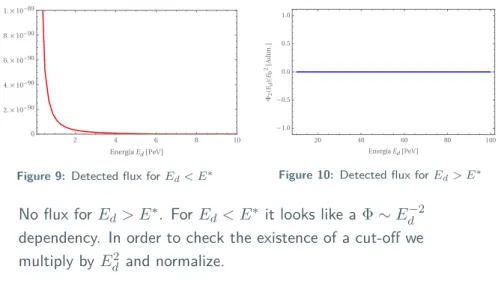
Figure 9:Detected flux forE_d< E^∗

20 40 60 80 100

-1.0 -0.5 0.0 0.5 1.0

EnergíaEd[PeV] Φ2(Ed)/E02[Adim.]

Figure 10: Detected flux forEd> E^∗

No flux forE_d> E^∗. For E_d< E^∗ it looks like aΦ∼E_d⁻² dependency. In order to check the existence of a cut-off we multiply byE_d² and normalize.

Bye, physics. Hi, computing

Now the cut-off is visible. We use log-scale in order to compare with Steckeret al. plots.

0 5 10 15 20

0.0 0.2 0.4 0.6 0.8 1.0 1.2

EnergíaE_d[PeV] Ed2·Φ(Ed)/Φ(1)[PeV2]

Figure 11: Analytic simulation of the flux

2 5 10

-1.5 -1.0 -0.5 0.0 0.5

EnergíaEd[PeV]

Log(Ed2·Φ(Ed)/Φ(1)[PeV2])

Figure 12:Logaritmic representation of the flux

Conclusion and discussion

Conclusion and discussion

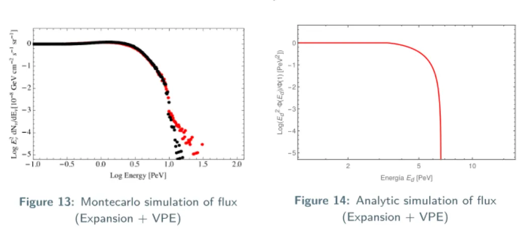
• We are able to recreate the expected cut-off:

Figure 13: Montecarlo simulation of flux (Expansion + VPE)

2 5 10

-5 -4 -3 -2 -1 0

EnergíaE_d[PeV]

Log(Ed2·Φ(Ed)/Φ(1)[PeV2])

Figure 14: Analytic simulation of flux (Expansion + VPE)

Conclusion and discussion

• The cut-off is produced by the existence of a limiting source z_c(E_d), which is the furthest source able to contribute to Φ(E_d).

1

(5 + 3n) Efd

−(5+3n)

−

∞ Eec−(5+3n)

!

= αn

3H₀ J(zc, z^∗)dt (20)

1 (5 + 3n)

1

E_d⁵⁺³ⁿ = αn

3H0

J(zc, z^∗)dt

Equation forzc(Ed) (21)

This critical distancezcis closer as Ed increases, so the number of sources contributing to the flux decreases quickly.

Conclusion and discussion

• The cut-off happen before the threshold energy E^∗, in a new scale energy which emerges naturally from the equations:

dEe

Ee⁶⁺³ⁿ = α_n 3H0

t^2/3+n

√Ωmt+ ΩΛ

dt → dEe

Ee = Ee⁵⁺³ⁿ 3H₀

α_n

j(t)dt ,

(22)

Defining the denominator as an energy:

En = 3H0

αn

_5+3n¹

→ dEe

Ee = Ee En

!⁵⁺³ⁿ

j(t)dt . (23)

Conclusion and discussion

• And this energy scale is always in the same order that the threshold energy.

E^∗ =4m²_eΛⁿ

1

2+n ∝ m²_eΛⁿ

1

2+n ∼ PeV (24)

En= (3H0/αn)⁵⁺³ⁿ¹ ∝ H0Λ³ⁿ/G²_F

1

5+3n ∼ PeV. (25)

Thanks for your attention!

There exist three different ways to approach to the problem of the abscence of neutrinos above2 PeV:

The cut-off in the detection spectrum is due to. . .

• . . .a cut-off in the emision spectrum.

Problem: There is not a cut-off in other messenger particles.

• . . .extrinsic propagation effects.

Problem: We need to identify the external entity and explain its opacity dependency with the energy.

• . . .intrinsic propagation effects.

Problem: Only exist one classical intrinsic effect. May need new physics.

Why Lorentz Invariance Violation?

New physics

Quantum Gravity

Space-Time modifications

Lorentz Invari- ance Violation

• We look for new physics.

• Quantum Gravity looks like a natural way.

• Gravity is related to the space-time.

• Lorentz Invariance reflects the structure of the space-time.

• CPT violation implies Lorentz Invariance violation (not in the other way).

We should characterize the distribution of sources.

Figure 15: Conical-trunk of trajectories of neutrinos

When the distance is large enough, the conical-trunk tends to a one-dimensional line. So we can characterize the distribution of sources as a one-dimentional functionf(z).

Possible sources: Active Galactic Nuclei (AGN) andγ-Ray Bursts (GRB). They are distributed according to the Star Formation Rate:

Figure 16: Star formation rate as a function ofz

In the casen= 1 (CPT-violating) theν are superluminical and the

¯ν not (or viceversa), so we do not have any cut-off:

Figure 17: Montecarlo simulations forn= 1

We call Glashow Resonance to the resonant formation of aW boson in antineutrino-electron collisions: ν¯e+e⁻ →W⁻.

Figure 18: Glashow resonance

Different diagrams for the Vacumm Pair Production.

The second one is only relevant 1/6 of all times. So theZ⁰ channel is the relevant one.

Figure 19: Vacumm Pair Production

Different diagrams for the Neutrino Splitting.

Figure 20: Neutrino Splitting

Figure 21: Screenshot of the script in Wolfram Mathematica

For more information you can google

“indicaciones de nueva física”: