Introduction to Lattice Field Theory

Introduction to Lattice Field Theory

P. Hernández (IFIC, UVEG-CSIC )

Plan

Part I: Functional Formulation of QFT, renormalization, Wilson RG Part II: Lattice Formulation of scalar, fermion and gauge QFT

Part III: Lattice QCD: numerical methods and applications

L. Lellouch et al. (ed.), Modern Perspectives in Lattice QCD: Quantum Field Theory and High Performance Computing. 93rd Session Les Houches International School

Oxford University Press 2011

C. Gattringer & CB Lang, QCD on the Lattice An Introduction for Beginners Springer Verlag 2009

T. DeGrand & C DeTar, Lattice Methods for Quantum Chromodynamics World Scientific 2006

HJ Rothe, Lattice Gauge Theories (3rd ed.) World Scientific 2005

J. Smit, Introduction to Quantum Fields on a Lattice Cambridge University Press 2002

[pioneer] M Creutz, Quarks, Gluons and Lattices Cambridge University Press 1983

Bibliography

Introduction

The Standard Model of particle physics has been tested sub % to be the theory describing microscopic particles and their interactions

SU (3) ⇥ SU (2) ⇥ U (1)

_Y

Elementary particle dynamics are accurately described by Quantum Field Theory (QFT).

LEP ⊕ flavour factories have established the Standard Model at 1% or better:

SM is a renormalizable QFT

L ^SM = L ^gauge + L ^matter + L ^SSB

L ^gauge = − 1

4g _U ² ₍₁₎ B _µν B _µν − 1

4g _SU ² ₍₂₎ W _µν W _µν − 1

4g _SU ² ₍₃₎ G _µν G _µν L ^matter = !

a

Ψ ¯ ^a i ̸ DΨ ^a

L ^SSB = !

ab

Ψ ¯ ^a Y _ab ΦΨ ^b + h.c. + L (Φ)

2

Gauge principle

Lepton<-> quark (anomaly cancellation)

(1,2) ¹

2 (3,2) ¹

6 (1,1) 1 (3,1) ²

3 (3,1) ¹

3

✓⌫e

e

◆

L

✓uⁱ dⁱ

◆

L

eR uⁱ_R dⁱ_R

✓⌫µ

µ

◆

L

✓cⁱ sⁱ

◆

L

µR cⁱ_R sⁱ_R

✓⌫⌧

⌧

◆

L

✓tⁱ bⁱ

◆

L

⌧R tⁱ_R bⁱ_R

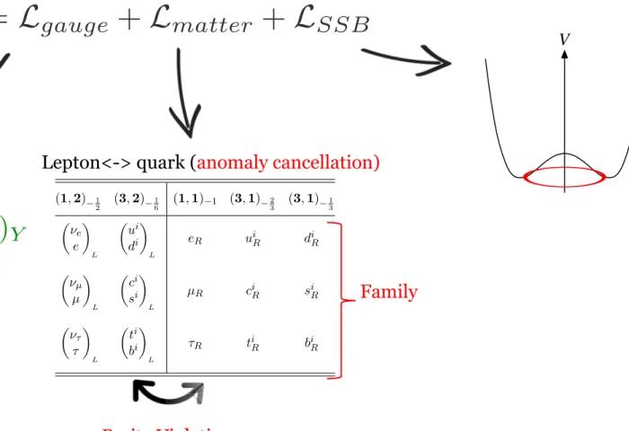
Table 1:Irreducible fermionic representations in the Standard Model: (dSU(3), dSU(2))Y

2 Neutrinos in the Standard Model

The Standard Model (SM) is a gauge theory based on the gauge groupSU(3)⇥SU(2)⇥U_Y(1). All elementary particles arrange in irreducible representations of this gauge group. The quantum numbers of the fermions(d_SU(3), d_SU(2))Y are listed in table 1.

Under gauge transformations neutrinos transform as doublets ofSU(2), they are singlets under SU(3)and their hypercharge is 1/2. The electric charge, given byQ=T3+Y, vanishes. They are therefore the only particles in the SM that carry no conserved charge.

The two most intriguing features of table 1 are its left-right or chiral asymmetry, and the three-fold repetition of family structures. Neutrinos have been essential in establishing both features.

2.1 Chiral structure of the weak interactions

The left and right entries in table 1 have well defined chirality, negative and positive respectively.

They are two-component spinors or Weyl fermions, that is the smallest irreducible representation of the Lorentz group representing spin1/2particles. Only fields with negative chirality (i.e. eigenvalue of

5minus one) carry theSU(2)charge. For free fermions moving at the speed of light (i.e., massless), it is easy to see that the chiral projectors are equivalent to the projectors on helicity components:

PR,L⌘ 1± 5

2 = 1 2

✓

1±s·p

|p|

◆

+O⇣mi

E

⌘

, (6)

where the helicity operator⌃= ^s_|^·_p^p_| measures the component of the spin in the direction of the momen- tum. Therefore for massless fermions only the left-handed states (with the spin pointing in the opposite direction to the momentum) carrySU(2)charge. This is not inconsistent with Lorentz invariance, since for a fermion travelling at the speed of light, the helicity is the same in any reference frame. In other words, the helicity operator commutes with the Hamiltonian for a massless fermion and is thus a good quantum number.

The discrete symmetry under CPT (charge conjugation, parity, and time reversal), which is a basic building block of any Lorentz invariant and unitary quantum field theory (QFT), requires that for any left-handed particle, there exists a right-handed antiparticle, with opposite charge, but the right-handed particle state may not exist. A Weyl fermion field represents therefore a particle of negative helicity and an antiparticle with positive one.

Parity however transforms left and right fields into each other, thus the left-handedness of the weak interactions implies that parity is maximally broken in the SM. The breaking is nowhere more obvious

4

Family

Parity Violation

Introduction Introduction to Weak Decays Goldstone Bosons Abelian Higgs Model SU(2)×U(1)

Goldstone Bosons – Continuous Symmetries Cont.

V

! The existence of Goldstone Bosons can be understood in terms of zero modes.

! O(N)has N(N−1)/2 generators and the residual symmetryO(N−1) has(N−1)(N−2)/2generators.

! The number of Broken Symmetries is therefore 1

2{N(N−1)−(N−1)(N−2)}=N−1 which is the number of Goldstone Bosons .

Standard Model SUSSP61, Lecture 1, 9th August 2006

Introduction

The Standard Model of particle physics has been tested sub % to be the theory describing microscopic particles and their interactions

SU (3) ⇥ SU (2) ⇥ U (1)

_Y

Elementary particle dynamics are accurately described by Quantum Field Theory (QFT).

LEP ⊕ flavour factories have established the Standard Model at 1% or better:

SM is a renormalizable QFT

L ^SM = L ^gauge + L ^matter + L ^SSB

L ^gauge = − 1

4g _U ² ₍₁₎ B _µν B _µν − 1

4g _SU ² ₍₂₎ W _µν W _µν − 1

4g _SU ² ₍₃₎ G _µν G _µν L ^matter = !

a

Ψ ¯ ^a i ̸ DΨ ^a

L ^SSB = !

ab

Ψ ¯ ^a Y _ab ΦΨ ^b + h.c. + L (Φ)

2

Gauge principle

Flavour Puzzle

Introduction

The Standard Model of particle physics has been tested sub % to be the theory describing microscopic particles and their interactions

Elementary particle dynamics are accurately described by Quantum Field Theory (QFT).

LEP ⊕ flavour factories have established the Standard Model at 1% or better:

SM is a renormalizable QFT

L

^SM

= L

^gauge

+ L

^matter

+ L

^SSB

L

^gauge

= − 1

4g

_U²₍₁₎

B

_µν

B

_µν

− 1

4g

_SU² ₍₂₎

W

_µν

W

_µν

− 1

4g

_SU² ₍₃₎

G

_µν

G

_µν

L

^matter

= !

a

Ψ ¯

^a

i ̸ D Ψ

^a

L

^SSB

= !

ab

Ψ ¯

^a

Y

_ab

ΦΨ

^b

+ h.c. + L (Φ)

2

Introduction

The Standard Model interactions imply a # of free parameters and accidental

symmetries: Most of the ugly/intriguing features of the SM are related to the SSB flavour sector that will be soon tested at the LHC:

Sector Free Param. Discrete Sym. Flavour Sym.

Gauge 3 C, P, T

Gauge+matter 3 T, C /, P/ U (N

_f

)

Gauge+matter+SSB 22-24 C /, P/, T/ U (1)

_B−L

or none

Most of what we can predict accurately in this model has been obtained in perturbation theory (PT)

3

+ A non-accidental “symmetry”: strong CP

L ^SM ✓ ¯ ↵ _s

8⇡ G G ˜ ✓ ¯  10 ¹⁰

Most of what we know is derived from perturbation theory and is not enough!

The need to go beyond perturbation theory

SU(3) interactions weak at large energies become strong at low energies

Growth of the coupling at low energies: Confinement

Generation of a mass gap Chiral symmetry breaking

Asymptotic freedom

FU

Static potential (potential between infinitely heavy quarks) grows with r:

Confinement

We do not observe asymptotic states with net color charge, only hadrons which are color singlets

V (r ) ⇠ r

Proton

Neutron string tension

FU

Mass gap

Light hadron masses (except pions) are dominated by the strong binding energy

m _proton

2m _u + m _d ⇠ 100

The mass of ordinary matter is mostly color binding energy!

One of the 6 Millennium Prize Problems still to be solved (1M$ prize!)

Yang–Mills Existence and Mass Gap. Prove that for any compact simple gauge group G, a non-trivial quantum Yang–Mills theory exists on R₄ and has a mass gap

∆ > 0. Existence includes establishing axiomatic properties at least as strong as those cited in [45, 35].

FU

Spontaneous Chiral Symmetry Breaking

The lightest pseudoscalar mesons are significantly lighter than the mass gap because they are Nambu-Goldstone bosons of chiral symmetry breaking

In the limit m

_u

=m

_d

= 0, there is a chiral global symmetry in QCD

Due to the strong interactions a quark condensate forms:

Spontaneous symmetry breaking:

h uu ¯ i = h dd ¯ i = ⌃ _ij

✓ u d

◆

L

! U

_L

✓ u d

◆

L

✓ u d

◆

R

! U

R

✓ u d

◆

R

SU (2) _L ⇥ SU (2) _R ! SU (2) _V

Three goldstone bosons: ⇡ ^± , ⇡ ⁰

FU

Chiral Symmetry Breaking

Goldstone theorem: hadron physics at low energies

Chiral symmetry of QCD spontaneously broken.

Hidden symmetry M _⇡ ⌧ M _nucleon

M _⇡ ² = (m _u + m _d ) |h 0 | (¯ uu + ¯ dd) | 0 i| 1 F _⇡ ²

Corrections due to non-vanishing Goldstone boson momenta and masses can be treated systematically through an effective description: Chiral Perturbation Theory.

expansion in p ²

⇤ ²

L = L ⁽²⁾ + L ⁽⁴⁾ + . . .

L ⁽²⁾ = F ²

4 Tr ⇥

@ _µ U ^† @ _µ U ⇤ ⌃

2 Tr h

e ^{i✓/N f} M U + h.c. i

L ⁽⁴⁾ = X

i

C ⁱ O ⁱ

[Nambu, Goldstone 1960-1]

[Gell-Mann, Oakes, Renner 1968]

[Weinberg 1979; Gasser, Leutwyler 1984-5]

[Gell-Mann, Oakes, Renner]

h 0 | A

^a_µ

(x) | ⇡

^a

(p) i = ip

_µ

F

_⇡

e

^ipx

, A

^a_µ

= ¯ Q

_{µ 5}

T

^a

Q

Light pseudoscalar mesons are very sensitive to light quark masses, the latter

can be extracted from the former

FU

Anomalous Chiral Symmetry Breaking

For m

u

=m

d

= 0 the symmetry group at the classical level also contains

However: there is no fourth goldstone boson: ⌘ ⁰

m _⌘

⁰

⇠ m _proton

@ _µ A ^µ = g ²

32⇡ ² G ^a _µ⌫ G ˜ ^a _µ⌫

The term on the right-hand side has no effect in perturbation theory, but

configurations exist that make this non vanishing beyond perturbation theory

U (1) _A broken by the anomaly:

[t’Hooft; Witten; Veneziano]

)2 (Q effα

2)

QCD(Q α

↑

confinement

2)

QED(Q α

asymptotic freedom →

↑Landau pole

) → large momentum transfer (Q2

probing small distance scales (x) →

Asymptotic freedom versus Landau Poles/Triviality

[↵(q)]

_QCD

⌘ g(q) ¯

²

4⇡ ⇠

^q!1

c

ln(

_⇤^q

) ^(Q

Landau Pole

)

_QED

= m

_e

exp

✓ 1

0

g(m ¯

_e

)

²

◆ b

₀

<0 Asymptotic Freedom b

₀

>0 Triviality and Landau Pole

(¯ q) = @ g ¯ (q)

@ ln q = ₀ g ¯ ³ + O (¯ g ⁵ )

The Standard Model at arbitrary high energy ?

1. Landau poles (perturbative) <-> triviality (non-perturbative)

2. Stability of the higgs potential <->

⇤ ! 1 :

_R

(µ) = 0, g

_1R

(µ) = 0

V ( ) = µ ^{2 †} + ( ^† ) ²

R (µ) > 0

The need to go beyond perturbation theory

3

rsta.royalsocietypublishing.orgPhil.Trans.R.Soc.A0000000...

0 50 100 150 200

0 50 100 150 200

Higgs mass M_h in GeV TopmassMtinGeV

Instability

Non-perturbativity

Stability Meta-stability

10⁷ 10⁸

10⁹

10¹⁰ 10¹¹ 10¹²

10¹³

10¹⁴

10¹⁶

120 122 124 126 128 130 132

168 170 172 174 176 178 180

Higgs pole massM_hin GeV ToppolemassMtinGeV

10¹⁷

10¹⁸

10¹⁹ 1,2,3s

Instability

Stability Meta-stability

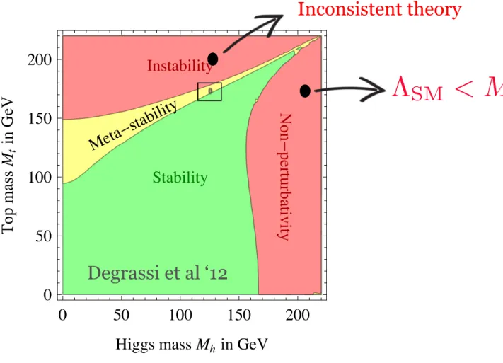
Figure 2. Different regions in the (M_h, Mt) plane concerning the structure of the Higgs potential at high field values:

stable (up to M_{P l}) in the green area; unstable in the yellow (red) areas above, with a lifetime of the EW vacuum longer (shorter) than the age of the Universe. In the sideband red region labelled “Non-perturbativity” in the left plot, the running hits a Landau pole below M_{P l}. Also shown are the 1-3 experimental ellipses, with M_h= 125.15±0.4 GeV and M_t = 173.34±0.76±0.3GeV. The left plot is from [3] and the right zoomed version from [4].

of interfering BSM physics) the EW vacuum would most likely be metastable, but with absolute stability excluded only at the 2-3 level,⁴ a result dubbed near-criticality. Fig. 3 shows the SM

“phase diagram” with different experimental ellipses: for different measurements of M_t, from ATLAS, CMS and the Tevatron (left plot) and for different combinations with updated data (right plot). Although the most realistic determination of the error inMtis still under debate (seee.g.[22]

for a review on the issues of the top mass determination), it will not change near-criticality.

Obviously, BSM physics can interfere with the running of the Higgs quartic coupling, disrupting the near-criticality shown in Fig. 2. This can happen even if the BSM physics is much heavier that the instability scale, provided the effect it has on the potential is to make it more unstable (pushing down the stability line in Fig. 2). A well-motivated example of this effect is heavy right-handed seesaw neutrinos with sizeable Yukawa couplings [6]; a less motivated example that has been widely discussed in the literature [23] is that Planckian physics might introduce additional sources of potential destabilization. (For a more detailed discussion of this, see [24]). In this respect, the hint of near-criticality might be compared with the hint of gauge coupling unification: both are easy to disrupt by new physics thresholds (in which case they are simply coincidences) but might be real hints pointing to some deeper and more fundamental theory.

This intriguing near-criticality has led to many theoretical speculations about its significance [4,8,25]. Is somehow (M_{P l})'0 connected to the fact that we also are very close to the phase boundary between the EW broken and unbroken phases? This second boundary is associated to the extreme smallness of the mass parameter of the Higgs potential, m², in Planck units:

m²/M_{P l}² ⇠0. From this point of view, it seems that the Higgs potential has a remarkable behaviour at the Planck scale, with and m² being both very small. Moreover, also has a special value '0 not very far from M_{P l}. Is there a deep reason why EW parameters take such intriguing values at M_{P l}, an scale related to gravitational physics rather than to EW physics? It is fair to say that no compelling theoretical explanation has been advanced so far.

4In Ref. [8], this number is reduced to⇠1.3 . However, comparison between the NNLO stability line of [3,4] and the refined result of [8] shows nearly perfect agreement. The discrepancy is simply due to the different choice of mass parameters in [8], namelyMt= 173.21±0.87GeV and, especially,Mh = 125.7±0.4GeV, see Fig.3, right plot.

The Standard Model is borderline OK up to the Planck scale but not beyond Degrassi et al ‘12

Intriguing correlation between SM pararameters: m

_t

, m

_h

, a

_s

!

⇤ _SM < M _P

Inconsistent theory

The (B)SM puzzles

i

• If there is new physics, there is a hierarchy problem

Solutions involve strong interactions: SUSY breaking, Technicolor, etc

• Flavoured new physics (e.g. FCNC) more strongly constrained than unflavoured ones:

Flavoured new physics in the quark sector involve strong interactions

• Strong CP problem…if CP is broken why not by QCD ?

H H

X

M _H ² / M _X ² log ⁰ s

✓F _µ⌫ ^a F ˜ ^aµ⌫

Term irrelevant in the perturbation theory

p ⇤

c [10

²

10

⁵

] TeV

Beyond PTh: Lattice Quantum Field Theory Lecture I: Functional formulation of Euclidean QFT, Regularization and Wilson RG

7

Basic idea due to K. Wilson: convert the path-integral formulation of a QFT into a statistical system by discretizing space-time

QCD and asymptotically free renormalizable theories are benchmarks

Lattice Quantum Field Theory

Lehman-Symanzik-Zimmerman Reduction Formula

Cross sections, decay widths <-> Field Correlation functions Lehman-Symanzik-Zimmerman Reduction Formula

Physical observables (cross sections, decay widths) ↔ Field correlation functions

!"#$%&'()"*

%&"+$*

!",-#&#$-* ./#,-#&#$-*

n

!

i=1

"

d⁴x_ie^ipi·xi

k

!

j=1

"

d⁴y_je^−iqj·yi⟨0|T #

φ(xˆ ₁)...φ(xˆ _n) ˆφ(y₁)....φ(yˆ _k)$

|0⟩

≃_p⁰

i→Epi,q0 j→Eqj

n

!

i=1

% i√

Z p²_i −m² + iϵ

& _k

!

j=1

% i√

Z q²_j −m² + iϵ

&

⟨p₁, ....,p_n, out|q₁, ...,q_k;in⟩,

Z , m one-particle field renormalization constant and mass ?

9

In-states Out-states

Interaction region

Lattice Quantum Field Theory

From Minkowski to Euclidean via a Wick rotation Wick rotation

Time-ordered correlation functions contain all the physical information of the theory

W

n

(t

1

, x

₁

; ...., t

n

, x

_n

) = ⟨ 0 | φ(t ˆ

1

, x

₁

)... φ(t ˆ

n

, x

_n

) | 0 ⟩ , t

1

≥ t

2

... ≥ t

n

, Can be continuously extended to analytic functions in the complex plane for

Imt

₁

≤ Im t

₂

≤ .... ≤ Im t

_n

The Schwinger functions or Euclidean correlation functions are defined as:

S

_n

(x

₁

, ..., x

_n

) = W

_n

( − ix

⁰₁

, x

₁

; ... − ix

⁰_n

, x

_n

), where the Euclidean times are x

⁰_i

= it

⁰_i

and

x

⁰₁

≥ x

⁰₂

.... ≥ x

ⁿ₀

.

11

Wick rotation

Time-ordered correlation functions contain all the physical information of the theory

W

_n

(t

₁

, x

₁

; ...., t

_n

, x

_n

) = ⟨ 0 | φ(t ˆ

₁

, x

₁

)... φ(t ˆ

_n

, x

_n

) | 0 ⟩ , t

₁

≥ t

₂

... ≥ t

_n

, Can be continuously extended to analytic functions in the complex plane for

Imt

₁

≤ Im t

₂

≤ .... ≤ Im t

_n

The Schwinger functions or Euclidean correlation functions are defined as:

S

_n

(x

₁

, ..., x

_n

) = W

_n

( − ix

⁰₁

, x

₁

; ... − ix

⁰_n

, x

_n

), where the Euclidean times are x

⁰_i

= it

⁰_i

and

x

⁰₁

≥ x

⁰₂

.... ≥ x

ⁿ₀

.

11

From quantum to classical variables: path integral representation

Lattice Quantum Field Theory

Characterization of asymptotic states (Z, m):

KL Spectral decomposition of the propagator in energy and momentum eigenstates

| a >

Dominated by the lowest energy states: one particle states

x

0

lim !1

Z

d ³ x h (x) (0) i / e ^m

^↵

^x

⁰

Lattice Quantum Field Theory

From functional integrals to multidimensional ordinary integrals via discretization of space-time

Lattice Scalar QFT

A scalar field in a discretized space-time, such as a cubic lattice:

φ(x) x = na n = (n

₀

, n

₁

, n

₂

, n

₃

) n

_i

∈ Z

⁴

.

!

dx

_i

→ a "

n_i∈Z

!

d

⁴

x → a

⁴

"

x

≡ a

⁴

"

n∈Z⁴

.

Any F (na) has a Fourier series periodic in the Brillouin zone (BZ):

F ˜ (p) = a

⁴

"

n

e

^−ipna

F (na) F ˜ (p) = ˜ F

#

p + 2π a m

$

, m ∈ Z

⁴

and

!

π/a

−π/a

d

⁴

p

(2π)

⁴

e

^ipna

F ˜ (p) = F (na).

41

Lattice Scalar QFT

A scalar field in a discretized space-time, such as a cubic lattice:

φ(x) x = na n = (n

₀

, n

₁

, n

₂

, n

₃

) n

_i

∈ Z

⁴

.

!

dx

_i

→ a "

n_i∈Z

!

d

⁴

x → a

⁴

"

x

≡ a

⁴

"

n∈Z⁴

.

Any F (na) has a Fourier series periodic in the Brillouin zone (BZ):

F ˜ (p) = a

⁴

"

n

e

^−ipna

F (na) F ˜ (p) = ˜ F

#

p + 2π a m

$

, m ∈ Z

⁴

and

!

π/a

−π/a

d

⁴

p

(2π)

⁴

e

^ipna

F ˜ (p) = F (na).

41

Lattice Scalar QFT

A scalar field in a discretized space-time, such as a cubic lattice:

φ(x) x = na n = (n

₀

, n

₁

, n

₂

, n

₃

) n

_i

∈ Z

⁴

.

!

dx

_i

→ a "

n_i∈Z

!

d

⁴

x → a

⁴

"

x

≡ a

⁴

"

n∈Z⁴

.

Any F (na ) has a Fourier series periodic in the Brillouin zone (BZ):

F ˜ (p) = a

⁴

"

n

e

^−ipna

F (na) F ˜ (p) = ˜ F

#

p + 2π a m

$

, m ∈ Z

⁴

and

!

π/a

−π/a

d

⁴

p

(2π)

⁴

e

^ipna

F ˜ (p) = F (na).

41

⇡

a $ momentum cuto↵

Lattice Quantum Field Theory

From functional integrals to multidimensional ordinary integrals via discretization of space-time

@

µ

(x) ! @ ˆ

µ

(x) ⌘ 1

a ( (x + aˆ µ) (x))

@ ˆ

_µ^⇤

(x) ⌘ 1

a ( (x) (x a µ)) ˆ

Any lattice derivative involves high dimension operators

@ ˆ

_µ

= @

_µ

+ 1

2 a@

_µ

@

_µ

+ O (a

²

)

Lattice Quantum Field Theory

Perturbative renormalizability: generic 1PI diagram in scalar lf

⁴

Perturbative renormalizability

The contribution of a 1PI diagram with I internal lines (i.e. propagators linking two vertices) and L loops is generically of the form:

Γ

^(N)

(p

₁

, ..., p

_N

) ∼

!

^L

"

l=1

d

⁴

q

_l

I

"

i=1

1

k

_i

(q

_l

, p

_j

)

²

+ m

²

.

Superficial degree of divergence: if q

_i

∼ Λ → Γ

^(N)

∼ Λ

^ω

ω ≡ 4L − 2I,

Negative ω is necessary for UV finiteness but not sufficient!

Topological relation between I , the number of vertices V and external legs N of the diagram:

2I + N = 4V,

24

! = superficial degree of divergence = 4L 2I

4V = N + 2I L = I V + 1

Using:

! = 4 N

Only N=2, 4 can be divergent

⁽²⁾

= A @

_µ

@

_µ

+ B

²

(4)

= C

⁴

Divergences in A, B, C can be reabsorbed in Z, m, l (proof to all others difficult!)

Lattice Quantum Field Theory

d>4 interactions

As more vertices of this type are included in a diagram higher N is necessary to absorb the divergence

More generically, we can consider a theory where S ⁽¹⁾ has other interactions such as

V ⁽¹⁾ [φ] = g _V (∂ ) ^N

^∂

(φ) ^N

^φ

ω = 4 − N − [g _V ]V, [g _V ] = 4 − N _φ − N _∂

A very different behaviour as the order of the perturbative expansion grows depending on the sign of [g _V ]:

[g _V ] > 0 diagrams become less divergent with V : superrenormalizable theory [g _V ] = 0 the divergence does not depend on V : renormalizable theory

[g _V ] < 0 divergences for larger N as V grows: non-renormalizable theory

The lattice formulation of any lattice field theory is not renormalizable in this sense....

26

More generically, we can consider a theory where S ⁽¹⁾ has other interactions such as

V ⁽¹⁾ [φ] = g _V (∂ ) ^{N ∂} (φ) ^{N φ}

ω = 4 − N − [g _V ]V, [g _V ] = 4 − N _φ − N _∂

A very different behaviour as the order of the perturbative expansion grows depending on the sign of [g _V ]:

[g _V ] > 0 diagrams become less divergent with V : superrenormalizable theory [g _V ] = 0 the divergence does not depend on V : renormalizable theory

[g _V ] < 0 divergences for larger N as V grows: non-renormalizable theory

The lattice formulation of any lattice field theory is not renormalizable in this sense....

26

More generically, we can consider a theory where S

⁽¹⁾

has other interactions such as

V

⁽¹⁾

[φ] = g

_V

(∂ )

^N∂

(φ)

^Nφ

ω = 4 − N − [g

_V

]V, [g

_V

] = 4 − N

_φ

− N

_∂

A very different behaviour as the order of the perturbative expansion grows depending on the sign of [g

_V

]:

[g

_V

] > 0 diagrams become less divergent with V : superrenormalizable theory [g

_V

] = 0 the divergence does not depend on V : renormalizable theory

[g

_V

] < 0 divergences for larger N as V grows: non-renormalizable theory The lattice formulation of any lattice field theory is not renormalizable in this sense....

26

Perturbative renormalizability:

More generically, we can consider a theory where S ⁽¹⁾ has other interactions such as

V ⁽¹⁾ [φ] = g _V (∂ ) ^N

^∂

(φ) ^N

^φ

ω = 4 − N − [g _V ]V, [g _V ] = 4 − N _φ − N _∂

A very different behaviour as the order of the perturbative expansion grows depending on the sign of [g _V ]:

[g _V ] > 0 diagrams become less divergent with V : superrenormalizable theory [g _V ] = 0 the divergence does not depend on V : renormalizable theory

[g _V ] < 0 divergences for larger N as V grows: non-renormalizable theory

The lattice formulation of any lattice field theory is not renormalizable in this sense....

26

Superrenormalizable Renormalizable

Non renormalizable

The lattice formulation is not renormalizable in this sense…

Wilsonian Renormalization

Consider a QFT with a fundamental cutoff

S

⇤

[ ] = Z

x

1

2 @

µ

@

µ

+ m

²

2

2

+ 4!

4

+

⁰

⇤

²

6

+ c

₂

⇤

²

@

⁴

+ ...

Z ⇤

⇤

dp

! = 4 N

w counts the powers of L

Exercise: show that

There is nothing special about a theory that is perturbatively renormalizable!

Wilsonian Renormalization

Renormalizability <-> existence of a continuum limit (criticality)

Continuum limit: a->0, keeping x fixed

⇠ = m

¹

a

h (x) (0) i / e ^x/⇠

Renormalizability is an emergent phenomenon in a theory with a fundamental cutoff (such as a lattice QFT ) ⇤ = a

¹

⇠

a ! 1 , ma ! 0

Empirical fact: many systems near critical points behave similarly (universality class)

Wilsonian Renormalization

Wilsonian Renormalizability:

S

⁽ⁿ⁾

(a) = !

i,x

g

_i⁽ⁿ⁾

O

_i

(x) S

⁽ⁿ⁺¹⁾

(a) = !

i,x

g

_i⁽ⁿ⁺¹⁾

O

_i

(x)

g

_i⁽ⁿ⁺¹⁾

= R

_i⁽ⁿ⁾

(g

⁽ⁿ⁾

) Fixed-points of RG: g

_i^∗

= R

_i

(g

^∗

)

m

_α

(g

^∗

) = fixed → m

_α

(g ∗ )a → 0

7

Wilsonian Renormalizability:

S

⁽ⁿ⁾

(a) = !

i,x

g

_i⁽ⁿ⁾

O

_i

(x) S

⁽ⁿ⁺¹⁾

(a) = !

i,x

g

_i⁽ⁿ⁺¹⁾

O

_i

(x)

g

_i⁽ⁿ⁺¹⁾

= R

⁽ⁿ⁾_i

(g

⁽ⁿ⁾

) Fixed-points of RG: g

_i^∗

= R

_i

(g

^∗

)

m

_α

(g

^∗

) = fixed → m

_α

(g ∗ )a → 0

7

Wilsonian Renormalizability:

S

⁽ⁿ⁾

(a) = !

i,x

g

_i⁽ⁿ⁾

O

_i

(x) S

⁽ⁿ⁺¹⁾

(a) = !

i,x

g

_i⁽ⁿ⁺¹⁾

O

_i

(x)

g

_i⁽ⁿ⁺¹⁾

= R

⁽ⁿ⁾_i

(g

⁽ⁿ⁾

) Fixed-points of RG: g

_i^∗

= R

_i

(g

^∗

)

m

_α

(g

^∗

) = fixed → m

_α

(g ∗ )a → 0

7

Renormalization group transformation

Renormalization group transformations

Let us suppose that we have a lattice scalar theory on a lattice of spacing a which describes physics scales m ≪ a

⁻¹

.

The most general local theory:

S (a) = !

α

g

_α

(a) !

x

O

_α

(φ(x), a)

where O

_α

are Lorentz invariant and local operators with arbitrary dimension constructed by powers of ∂

_µ

φ, φ and a.

Take the limit a → 0 in little steps:

a ≥ a

₁

≥ a

₂

... ≥ a

_n

= (1 − ϵ)

ⁿ

a, ϵ ≪ 1

At each step we can integrate the modes between a

⁻_n−¹₁

and a

⁻_n¹

to obtain an effective

29

At each step we integrate the modes [a _n ¹ ₁ , a _n ¹ ]

Wilsonian Renormalization

At each step we integrate the modes to match to a theory with the same cutoff [a _n ¹ ₁ , a _n ¹ ]

theory at a lower scale:

S (a

₁

) → S

⁽¹⁾

(a) = !

α

g

_α⁽¹⁾

(a) !

x

O

_α

(φ(x), a)

S (a

₂

) → S

⁽¹⁾

(a

₁

) → S

⁽²⁾

(a) = !

α

g

_α⁽²⁾

(a) !

x

O

_α

(φ(x), a)

....

S (a

_n

) → .... !

α

g

_α⁽ⁿ⁾

(a) !

x

O

_α

(φ(x), a)

The operators at scale a are all the same because we included all possible

Renormalization group (RG) transformation, the function that defines the change in the couplings:

R

_α

: g

_α⁽ⁿ⁾

→ g

_α⁽ⁿ⁺¹⁾

g

_α⁽ⁿ⁺¹⁾

= R

_α

(g

⁽ⁿ⁾

)

For a continuous transformation there is a RG flow of the coupling constants

30

Fixed Point of RG

Wilsonian Renormalizability:

S

⁽ⁿ⁾

(a) = !

i,x

g

_i⁽ⁿ⁾

O

_i

(x) S

⁽ⁿ⁺¹⁾

(a) = !

i,x

g

_i⁽ⁿ⁺¹⁾

O

_i

(x)

g

_i⁽ⁿ⁺¹⁾

= R

⁽ⁿ⁾_i

(g

⁽ⁿ⁾

) Fixed-points of RG: g

_i^∗

= R

_i

(g

^∗

)

m

_α

(g

^∗

) = fixed → m

_α

(g ∗ )a → 0

7

Wilsonian Renormalizability:

S

⁽ⁿ⁾

(a) = !

i,x

g

_i⁽ⁿ⁾

O

_i

(x) S

⁽ⁿ⁺¹⁾

(a) = !

i,x

g

_i⁽ⁿ⁺¹⁾

O

_i

(x)

g

_i⁽ⁿ⁺¹⁾

= R

_i⁽ⁿ⁾

(g

⁽ⁿ⁾

) Fixed-points of RG: g

_i^∗

= R

_i

(g

^∗

)

m

_α

(g

^∗

) = fixed → m

_α

(g ∗ )a → 0

7

Wilsonian Renormalization

Renormalizability <-> Universality Fixed Point of RG

Near a FP:

Near a fixed-point the evolution of the couplings reads at linear order

g

_α⁽ⁿ⁺¹⁾

− g

_α^∗

= ∂ R

_α

∂ g

_β

!

!

!

!

g^∗

(g

_β⁽ⁿ⁾

− g

_β^∗

),

so the distance to the fixed-point ∆g

⁽ⁿ⁾

changes according to the following equation:

∆g

_α⁽ⁿ⁺¹⁾

= M

_αβ

∆g

_β⁽ⁿ⁾

, M

_αβ

≡ ∂ R

_α

∂ g

_β

!

!

!

!

g^∗

.

We can find different situations depending on the eigenvalues, λ, of the matrix M :

λ > 1 ∆g

α⁽ⁿ⁾

increases as n → ∞ α is a relevant direction λ = 1 ∆g

_α⁽ⁿ⁾

stays the same as n → ∞ α is a marginal direction λ < 1 ∆g

_α⁽ⁿ⁾

decreases as n → ∞ α is an irrelevant direction

32

Near a fixed-point the evolution of the couplings reads at linear order

g

_α⁽ⁿ⁺¹⁾

− g

_α^∗

= ∂ R

_α

∂ g

_β

!

!

!

!

g^∗

(g

_β⁽ⁿ⁾

− g

_β^∗

),

so the distance to the fixed-point ∆g

⁽ⁿ⁾

changes according to the following equation:

∆g

_α⁽ⁿ⁺¹⁾

= M

_αβ

∆g

_β⁽ⁿ⁾

, M

_αβ

≡ ∂ R

_α

∂ g

_β

!

!

!

!

g^∗

.

We can find different situations depending on the eigenvalues, λ, of the matrix M :

λ > 1 ∆g

α⁽ⁿ⁾

increases as n → ∞ α is a relevant direction λ = 1 ∆g

_α⁽ⁿ⁾

stays the same as n → ∞ α is a marginal direction λ < 1 ∆g

_α⁽ⁿ⁾

decreases as n → ∞ α is an irrelevant direction

32

Different situations depending on eigenvalues of M

Near a fixed-point the evolution of the couplings reads at linear order

g

⁽ⁿ⁺¹⁾_α

− g

_α^∗

= ∂ R

_α

∂ g

_β

!

!

!

!

g^∗

(g

_β⁽ⁿ⁾

− g

_β^∗

),

so the distance to the fixed-point ∆g

⁽ⁿ⁾

changes according to the following equation:

∆g

_α⁽ⁿ⁺¹⁾

= M

_αβ

∆g

_β⁽ⁿ⁾

, M

_αβ

≡ ∂ R

_α

∂ g

_β

!

!

!

!

g^∗

.

We can find different situations depending on the eigenvalues, λ, of the matrix M :

λ > 1 ∆g

α⁽ⁿ⁾

increases as n → ∞ α is a relevant direction λ = 1 ∆g

α⁽ⁿ⁾

stays the same as n → ∞ α is a marginal direction λ < 1 ∆g

_α⁽ⁿ⁾

decreases as n → ∞ α is an irrelevant direction

# of relevant directions is usually small: universality & renormalizability

32

Wilsonian Renormalizability:

S

⁽ⁿ⁾

(a) = !

i,x

g

_i⁽ⁿ⁾

O

_i

(x) S

⁽ⁿ⁺¹⁾

(a) = !

i,x

g

_i⁽ⁿ⁺¹⁾

O

_i

(x)

g

_i⁽ⁿ⁺¹⁾

= R

⁽ⁿ⁾_i

(g

⁽ⁿ⁾

) Fixed-points of RG: g

_i^∗

= R

_i

(g

^∗

)

m

_α

(g

^∗

) = fixed → m

_α

(g ∗ )a → 0

7

Exercise: convince yourself that a free massless scalar is a fixed point (gaussian fixed point)

Start with a generic lattice action quadratic in the fields but otherwise arbitrary Case 2: We start with an arbitrary lattice action that is quadratic in the fields, but including all terms that are Lorentz invariant.

S (a) =

!

BZ(a)

d

⁴

p (2π)

⁴

1

2 φ( − p)

"

p

²

+ m

²₀

1

a

²

+ g

₁

a

²

p

⁴

+ ...

#

φ(p)

[m

₀

] = [α] = ... = 0.

the integration over the momentum modes in a slice of momenta in BZ (a

₁

) and out of BZ (a) can be done as before

S

⁽¹⁾

(a) =

!

BZ(a)

d

⁴

p (2π)

⁴

1

2 φ( − p)

$

p

²

+

"

a a

₁

#

2

1

a

²

m

²₀

+ g

₁

% a

₁

a

&

2

a

²

p

⁴

+ ...

'

φ(p),

35

(i) Construct the effective action

Case 2: We start with an arbitrary lattice action that is quadratic in the fields, but including all terms that are Lorentz invariant.

S (a) =

!

BZ(a)

d

⁴

p (2π)

⁴

1

2 φ( − p)

"

p

²

+ m

²₀

1

a

²

+ g

₁

a

²

p

⁴

+ ...

#

φ(p)

[m

₀

] = [α] = ... = 0.

the integration over the momentum modes in a slice of momenta in BZ (a

₁

) and out of BZ (a) can be done as before

S

⁽¹⁾

(a) =

!

BZ(a)

d

⁴

p (2π)

⁴

1

2 φ( − p)

$

p

²

+

"

a a

₁

#

2

1

a

²

m

²₀

+ g

₁

% a

₁

a

&

2

a

²

p

⁴

+ ... '

φ(p),

35

(ii) Construct the matrix M from this one step and find the relevant, irrelevant and marginal directions

The fact that the number of relevant directions is finite and usually small is behind the two related properties: universality of the fixed-point and the renormalizability of the corresponding QFT.

Example: Gaussian Fixed Point

Case 1: the free massless point of a scalar theory is a fixed-point:

S (a) =

!

BZ(a)

d

⁴

p (2π)

⁴

1

2 φ( − p)p

²

φ(p),

where BZ (a) is the Brillouin zone [ − π/a, π/a] in each mometum direction.

When we do the first RG transformation we start with the same action but in a lattice of spacing a

₁

= (1 − ϵ)a. Since the fields at different momenta are independent variables, we can integrate over those at momenta π/a ≤ | p

_µ

| ≤ π/a

₁

so that the

33

Wilsonian Renormalization

Any local action with the same degrees of freedom and symmetries lead to

the same continuum limit (via the tuning of a small set of relevant parameters) Asymptotic freedom ensures the existence of FP in perturbation theory

QCD has the (marginally) relevant couplings: g

₀

, m

_u

,m

_d

,m

_s

,m

_c

,…

Wilsonian Renormalizability:

Critical Regions ↔ Effective QFT

Fixed Points ↔ Renormalizable QFT: continuum limit Universality ↔ small number of relevant directions

Universality of the FP ensures that any discretization leads to the same continuum limit if the same properties concerning

• degrees of freedom

• locality

• symmetries

In asymptotically-free theories (QCD) the existence of a FP is warrantied by asymptotic freedom: can be proven in lattice perturbation theory!

Unitarity can be warrantied by the property of reflection positivity

Osterwalder, Seiler

8

g

0

->0 , m

_q

a -> 0

Caveat: a discretization that breaks any of the symmetries in general requires

more relevant couplings