What you will see in the various chapters of these notes actually represents how I perceive computational physics should be taught. We will also present some of the most popular algorithms from numerical mathematics that are used to solve a multitude of problems in the sciences. In almost every case, the algorithm you end up writing reflects your own understanding of the physics and mathematics (the way you express yourself) of the problem.
In several projects, we hope to present some more 'realistic' examples to solve with different numerical methods. When you access the course website, you will notice that you can obtain all the source files for the programs discussed in the text.
Introduction to Numerical Methods in Physics
Introduction
The fast Multipole algorithm, developed by Leslie Greengard and Vladimir Rokhlin; (calculating gravitational forces in an N-body problem usually requires N2 calculations. The fast multipole method uses order N calculations, approximating the effects of groups of distant particles using multipole expansions). In chapter 12, we deal with proprietary systems and applications for e.g. The Schrödinger equation rewritten as a matrix diagonalization problem. More detailed aspects of the above two programming languages will be discussed in the laboratory classes and various chapters of this text.
If speed is an issue, one can port critical parts of the code to Fortran 77. It is crucial to have a logical structure of e.g. the flow and organization of data before you start writing.
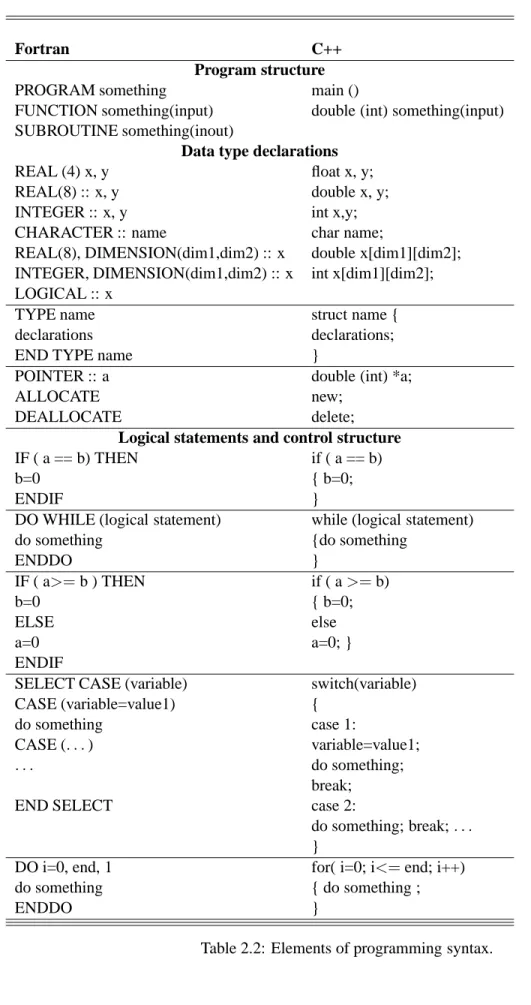
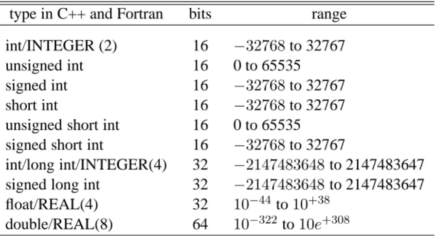
Introduction to C++ and Fortran
The asterisks (*,*) after WRITE represent the default format for output, i.e. the output is e.g. written on the screen. Since the typical computer communicates with us in the decimal system, but operates internally in, say, the binary system, conversion procedures must be performed by the computer, and these conversions hopefully involve only small rounding errors. In the following example, we assume that we can only represent a floating point number with a precision of 5 digits to the right of the decimal point.
The mantissa contains the significant digits of the number (and therefore the precision of the number). To describe an atom like Neon, we would need three single-particle orbits to describe the ground state wavefunction if we use a single-particle image, i.e. the 1s, 2s and 2p single-particle orbits.
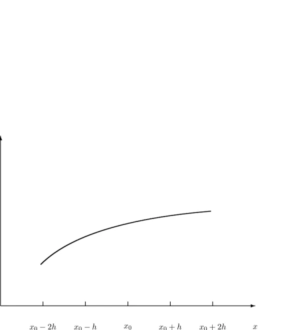
Numerical differentiation
However, we use call by value when the called function simply receives the value of the given variable without changing it. Two properties are important for these locations - address in memory and content in. In the C programming language, it is expressed as a modification of the value pointed to by y, namely the first element b.
The way the program is presented here is somewhat impractical, as we have to recompile the program if we want to change the name of the output file. Since this is a generic method, its functionality could be extended by simply passing in the name of the distinguishing function.
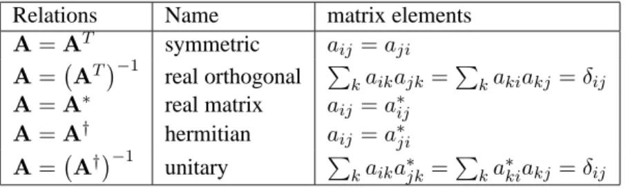
Linear algebra
The rest of the main() function is as in the previous example until line f. Here we have a call to a user-defined function that frees the reserved array memory. This means that the size of the array can change during program execution.
In this section, we describe some of the most commonly used algorithms for solving sets of linear equations. In the discussion, we again restrict ourselves to the matrix A∈R4×4, which results in a set of linear equations of the form. With n−1 such eliminations, we get the so-called upper triangular set of equations of the form.
In partial or column pivoting, we rearrange the rows of the matrix and the right side to bring the numerically largest value in the column onto the diagonal. Here are the unknowns eru12,u22,l32andgl42, all of which can be evaluated using the results from the first column and the elements of A. The Cholesky decomposition algorithm is a special case of the general LU decomposition algorithm.
This function returns the LU-decomposed matrix A, its determinant, and the vector index that keeps track of the number of interchanges of rows. We use this form since the calculation of the inverse goes through the inverse of the matrices L and U. Similarly, we can define an equation which gives us the inverse of the matrix U, labeled E in the equation below.
This only contains non-zero matrix elements in the upper part of the matrix (plus the diagonal). with the following general equation. Show that you can rewrite this equation as a linear set of equations of the form Av= ˜b,.
Non-linear equations and roots of polynomials
Solving an equation of the type f(x) = 0 means mathematically finding all numbers s1 such that f(s) = 0. Now we can formulate sufficient conditions for the convergence of the iterative search for solutions to f(s) = 0. Since it is difficult to numerically find the exact point , where f(s) = 0, we perform three type tests in the actual numerical solution.
Note that this convergence criterion is independent of the actual function f(x) as long as this function satisfies the conditions discussed in the conditions discussed in the previous subsection. In this function we transfer the lower and upper bounds of the interval where we are looking for the solution, [x1, x2]. Also note that this function passes a pointer to the name of the given function throughdouble(∗func ) (double).
In this sense it is adapted to cases with e.g. transcendental comparisons of the type shown in Eq. 5.8) where it is quite easy to evaluate the derivative. We again transfer the lower and upper limit of the interval where we are looking for the solution, [x1, x2] and the variablexa. We can run the risk of holding one of the endpoints while the other only slowly converges to the desired solution.
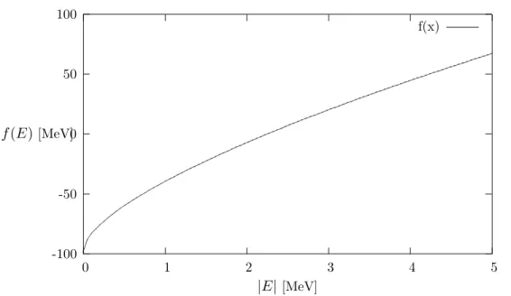
A variation of the secant method is the so-called false position method (regula falsi from the Latin) where the interval [a,b] is chosen such that f(a)f(b) < 0, otherwise there is no solution. We will study the solution of the Schrödinger equation (SE) for a system with a neutron and proton (deuteron) moving in a simple box potential. We begin our discussion of SE with the neutron-proton (deuteron) system with a box potential V(r).
Numerical interpolation, extrapolation and fitting of data
The function ωN+1(x) is given by. x−xN), (6.8) andξ=ξ(x)is a point in the smallest interval containing all interpolation points xjandx. This corresponds to the coefficienta1 and the tabulated value fx0x1 and together meta0 results in the polynomial for a straight line. The POLINT function in the library is based on an extension of this algorithm, known as Neville's algorithm.
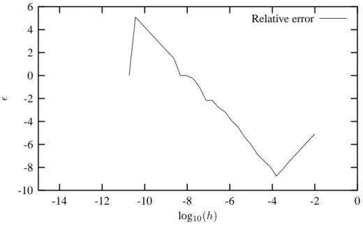
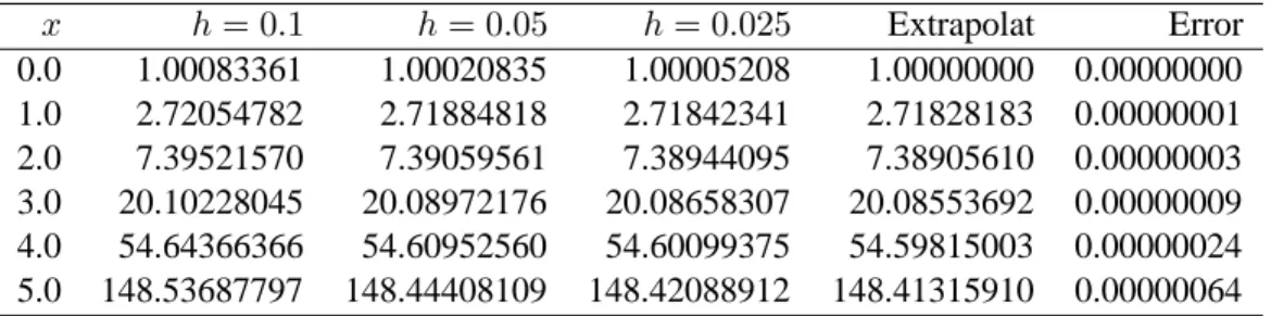
We will again study the evaluation of the first and second derivatives of exp (x) at a given point x=ξ. 3.3) and (3.4) for the first and second derivatives, we noticed that the truncation error goes asO(h2j). By applying the midpoint approximation to the derivative, the various derivatives Daf a given functionf(x) can then be written as. 6.20) where D(h) is the calculated derivative, D(0) the exact value in the limit → 0 and is independent of h. But since the derivatives involve differences, we can easily lose numerical precision as shown in the previous sections.
A possible cure is to apply Richardson's deferred approach, i.e., we perform the calculations with several values of the step and extrapolate toh = 0. The philosophy is to combine different values of th so that the terms in the above equation include only large exponents. To see this, suppose we assemble a calculation for two values of the step h, one withh and the other withh/2.
In Table 3.1 we presented the results for various step sizes for the second derivative of exp (x) using f0′′ = fh−2fh02+f−h. The extrapolated result toh= 0 must then be compared with the exact one from Table 3.1. method to obtain improved eigenvalues in chapter 12. Qubic spline interpolation is one of the most commonly used methods for interpolating between data points where the arguments are organized as ascending series. In the library program we provide such a function, based on the so-called qubic spline method described below.
Numerical integration
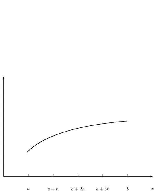
Note that the improved accuracy in evaluating the derivatives gives a better error approximation, O(h5) vs. The importance of using orthogonal polynomials in the evaluation of integrals can be summarized as follows. The mesh points are the zeros of the chosen orthogonal polynomial of order N, and the weights are determined from the inverse of a matrix.
Note that we have chosen to number the points from 0 to N − 1. Using the orthogonality property of the Legendre polynomials, we have Z 1. Instead of an integration problem, we now have to define the coefficient α0. To verify that the new weights are correct, remember that the weights must match the derivative of the net points.
The polynomials then form the basis for the Gauss-Laguerre method which can be applied to form integrals. It means that the curve1/(s) has equal and opposite areas on both sides of the singular points = 0. In choosing the grid points for a PV integral, it is important to use an even number of points, since an odd number of grid points always pickssi = 0as one of the grid points.
Specifically, we'll introduce you to using the Message Passing Interface (MPI) library. The MPI_COMM_RANK function returns the rank (the name or identifier) of the tasks that execute the code. Increasing should of course increase the accuracy of the result, as discussed at the beginning of this chapter.
Outline of the Monte-Carlo strategy
8.2) The numbers in the domain are the results of the physical process of rolling the dice. We first define the variance of the integral to be a uniform distribution on the intervalx∈[0,1]. We note that the standard deviation is proportional to the inverse square root of the number of measurements.
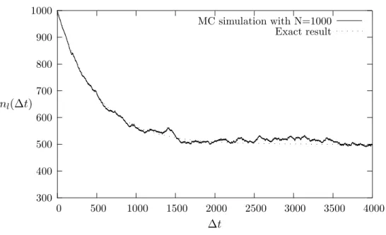
All random number generators produce pseudo-random numbers in the interval [0,1] using the so-called uniform probability distribution p(x) defined as . Radioactive decay is one of the classic examples of using Monte Carlo simulations. We have already seen the use of the last equation when we applied the rough Monte Carlo approximation to the evaluation of an integral.
Let's recap some of the above concepts using a discrete PDF (which is what we end up doing on a computer anyway). Typical periods for the random generators in the program library are on the order of ~109 or larger. The independence of the random numbers is crucial in the assessment of other expected values.
In quantum mechanics, the probability distribution function is given by p(x) = Ψ(x)∗Ψ(x), where Ψ(x) is the eigenfunction resulting from the solution of, for example, the time-independent Schrödinger equation. But if we have made a smart choice for Ψ(x), the expression H(x)˜ shows smooth behavior close to the exact solution. In the function that sets the integral, we just need to call one of the random number generators like ran0, ran1, ran2 or ran3 to get numbers in the interval [0,1].