Linear calibration using reference materials

Figure 2—Schematic diagram of a calibration curve 6 Figure 3 —Schematic diagram of placement of residuals versus fitted values 6 Figure 4 —Schematic diagram of a control chart to validate the calibration curve under the assumption of constant residual standard deviation 12 Figure 5 —Schematic diagram of the data calibration point. Draft International Standards adopted by the technical committees are circulated to the member bodies for voting. Publication as an International Standard requires approval by at least 75% of the member bodies voting. The following standards contain provisions which, by reference in this text, constitute provisions of this International Standard. At the time of publication, the indicated editions were valid. All standards are subject to revision, and parties to agreements based on this International Standard are encouraged to investigate the possibility of applying the most recent editions of the standards indicated below.

The procedure in this International Standard applies only to measurement systems that are linearly related to their reference systems. To check if the assumption of linearity is valid, more than two RMS should be used during the calibration experiment. This is illustrated in the basic method. Using several RMs, the basic method provides a strategy and techniques to analyze the data collected during the calibration experiment. If linearity is not an issue, an alternative method, simpler than the basic method, can be used to estimate linear calibration function based on one point. This "one-point calibration" method (after zero-level transformation) does not allow any testing of assumptions, but it is a quick and easy method to "recalibrate" a system that has been studied more thoroughly during previous experiments. If linearity is in question, a second alternative can be used, called "brackets". The basic method and the one-point method are based on the assumption that the effort invested in calibration will be valid over a period of stability of the process. To study the period over which the calibration is valid, a control method must be in place. The control method is designed to determine if changes have occurred in the system that warrant an investigation and/or calibration.

The control method also provides a simple way to determine the accuracy of the values transformed with a given calibration function. The bracket method is labor intensive, but can provide greater accuracy in determining the values of unknown quantities. This method consists of surrounding each unknown quantity as closely as possible (brackets) by two RMs and extracting a transformed value for the unknown quantity from measurements of both the unknown quantity and the values of the two RMs. Only short-term stability of the measurement process is assumed (stability during the measurement of the unknown quantity and of the two RMs). Linearity is assumed exclusively in the interval between the values of the two RMs.

Calibration experiment .1 Experimental conditions

Strategy for analysing the data .1 Plot the data to check

6 The steps of the basic method

Plot of the data collected during the calibration experiment
Estimation of the linear calibration function under the assumption of constant
Plots of the calibration function and of the residuals
Estimation of the calibration function under the assumption of proportional
Evaluation of the lack of fit of the calibration function

Model with proportional residual standard deviation (defined in 6.4)

Transformation of future measured values with the calibration function

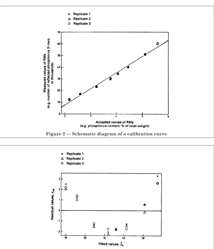
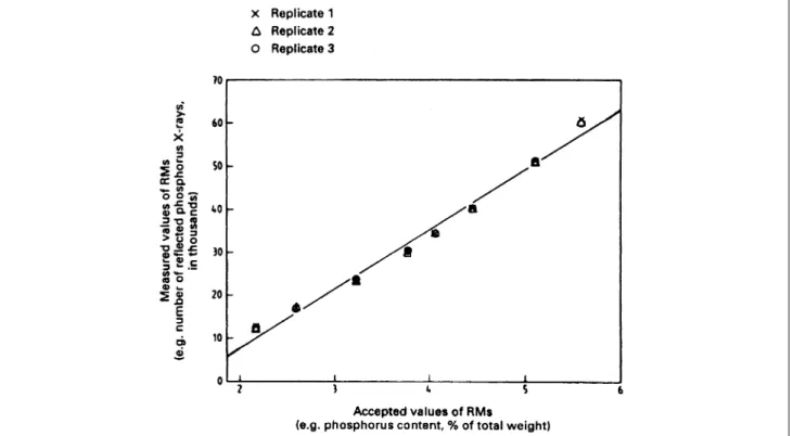
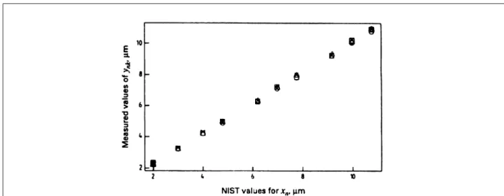
Estimates of the parameters b0,b1andgs2 can be obtained using the formulas below or by running a linear regression software package with two columns of equal length, one fory and one forx. The plot shown in Figure 2 primarily allows a check of the calculations given in 6.2.2. It also provides a visual check of the linearity assumption of the calibration function. The plot of the residuals enk versus the fitted values (Figure 3) is an effective tool for detecting deviation from the two assumptions of linearity and constant residual standard deviation.

If these two assumptions hold, Figure 3 should show a plot of randomly distributed points centered around zero. Deviation from the assumption of linearity is indicated by a systematic pattern between the residuals and the fitted values (such as the example in Figure 3). Deviation from the assumption of a constant residual standard deviation is indicated by dispersion in the data that increases or decreases with adjusted values. In Figure 3, the dispersion of the residuals for any fitted value is almost always constant. Therefore, the assumption of a constant standard deviation of the residual is tenable in this situation. If the assumption of a constant residual standard deviation does not hold, the data collected during the calibration experiment must be reanalyze. A plot of the standard deviation of repeated measurements of the RM versus the accepted value of that RM will indicate whether the assumption of a proportional residual standard deviation is acceptable. See Figure 9 for such a graph. a) If the proportional residual standard deviation assumption appears to hold, the data can be reanalyzed according to step 6.4. b) If the assumption of a proportional residual standard deviation does not hold, but there is a model that relates the residual standard deviation to the accepted RM values (for example, inverse proportionality), an approach similar to that presented in step 6.4 can be used. Finally, testing the assumptions of independence and normality of εnk values is beyond the scope of this International Standard. These two assumptions are key to the validity of step 6.5 and can also be verified by examining the residuals.

The estimates of the parameters y0,y1andτ2can be obtained by using the formula below or by running a weighted linear regression software package with three columns of equal length as input, one fory, one forx and one for the weights ( = 1/ x2). The same output can also be obtained by using a linear regression software package without weights but with the two input columns sandw. Where. As in 6.3, two plots are recommended: . a) a plot of the estimated calibration function using the data from Figure 1; .. b) a plot of the weighted residuals unk versus the weighted adjusted values. The selection of the significance level depends on specific applications and is left to the user of this international standard.

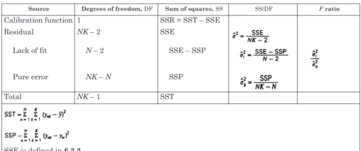
F(1 –α)(N– 2; NK–N), then there is no evidence to reject the linear model. b) If it is greater than F(1 –α)(N– 2; NK–N), then potential causes for large variability due to lack of fit relative to pure error variability should be investigated. A common cause is the inadequacy of the linear assumption of the calibration function (see Figure 2 and Figure 3). If the proportional residual standard deviation model was used, the ANOVA table is constructed as shown in Table 2. Transforming these measured values will result in a single value that estimates the true value of the unknown quantity. The transformation depends on the assumption made regarding the residual variance and is .

Table 2 - ANOVA table comparing lack of fit and pure error assuming proportional non-normal standard deviation.

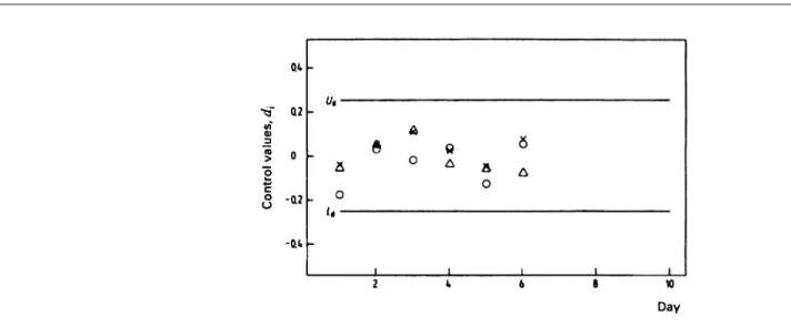
7 Control method

General
Calculation of upper and lower control limits

Model with proportional residual standard deviation

Collection and plotting of the data

Obtain the transformed values of each one of these m RMs (see 6.6). These transformed values

Decision about the state of the system If one or more values of d i falls outside the control
Estimation of the uncertainty of the transformed values

Model with proportional residual standard deviation

Table 2—ANOVA table for comparing lack of fit and pure error under the assumption of proportional residual standard deviation .. b) Plot the limits UdLon the control chart. If the calibration model assumes proportional residual standard deviation, the differences are normalized by dividing them by xi. Let the resulting values be referred to as the control values where. The same conclusions are reached for the proportional residual standard deviation model by comparing the ci values with the limits UcandLc.

For the calibration function subject to the control method, the uncertainty of the transformed values is approximated by the combined variance of the control values of two RMs (of which the RMs are selected for the control method): the RM with the minimum and maximum value. This is explained by the fact that the transformed values are expected to have more variance at the end of the range of values found during the calibration experiment than those in the middle of that range. Thus, the confidence interval for the transformed value derived from the variability of the two extreme RMs is approximately correct for values at the end of the application range and conservative for values in the middle of that range. Let dljanddmj be the control value of the minimum and maximum RM, where jrepresents the time during which the measurements were made. Then, during the periodJ of times when the measuring system is in a state of statistical control, the standard. Let cljandcmj be the control values of the minimum and maximum RM, where jrepresents the time during which the measurements were made. Then, during the J period of time when the measurement system was in the state of statistical control, the coefficient of variation of the transformed value is approximately estimated by.

To ensure that the variability due to the calibration procedure is included in the uncertainty statement, choose one set of control values (dlj,dmj) or (clj,cmj) from each calibration interval and use the same formula for or , where this is now the number of recalibrations.

8 Two alternatives to the basic method

General

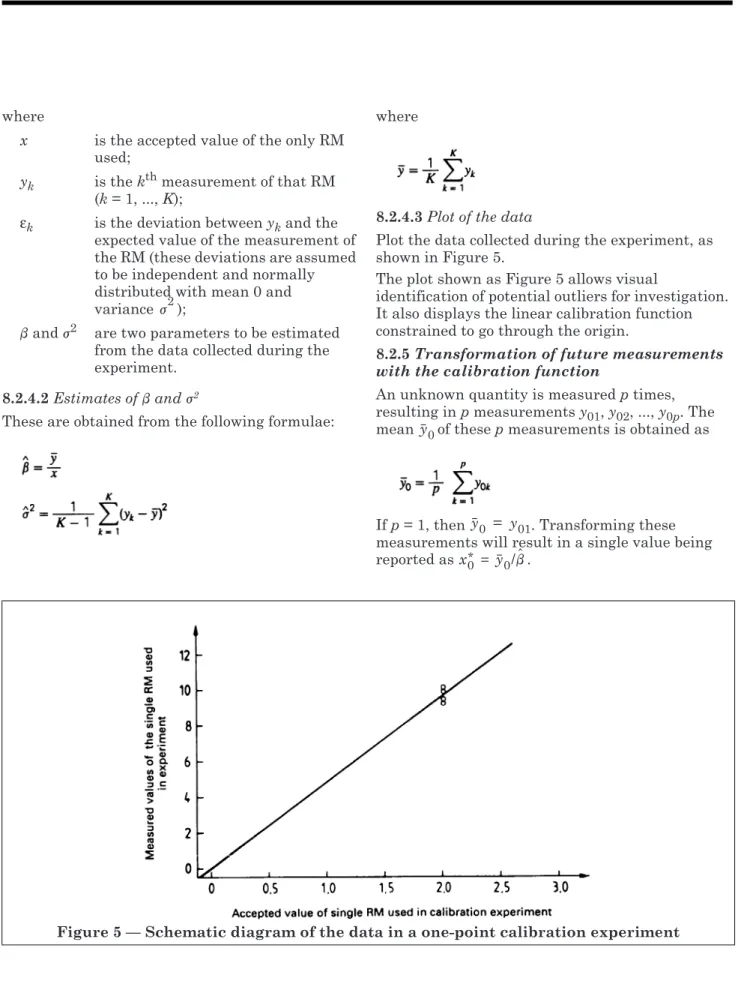
One-point calibration method .1 General

Assumptions It is assumed that
One-point calibration experiment a) Experimental conditions; the experimental

NOTE 8 In principle, the gap does not always have a true value of 0, but instead has an accepted value of xb, known to measure yb. If not negligible, the one-point calibration method described in 8.2.3 may be used with the following adjustments. . a) Measure the gap and adjust the numbers of the measuring instrument to the ready. . b) Measure the single RM used, as in the case of a blank with a value of 0. . c) The model becomes . d) The evaluation is done. e) The is2 estimate is unchanged. . f) The estimation of the true value of an unknown quantity measured p times (y01,y02,..,y0p) is.

Bracketing technique .1 General

Assumptions
Bracketing experiment

In principle, the blank does not always have a true value of 0, but instead has an accepted value of xb, which is known to have some degree of yb. If this is not negligible, the one-point calibration method described in 8.2.3 can be used with the following adjustments. . a) Measure the blank and adjust the pointers of the measuring instrument to readyb. . b) Measure the only RM used, as in the case of a blank with value 0. . c) The model becomes . d) The estimate of becomes . e) The estimate of s2 is unchanged. . f) The estimate of the true value of an unknown quantity measured p times (y01,y02,..,y0p) is.

9 Example

General

Basic method

Plot of the data
Evaluation of the lack of fit of the calibration function
Tranformation of future measurements Based on the calibration function obtained in 6.4,

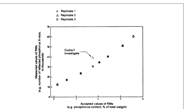
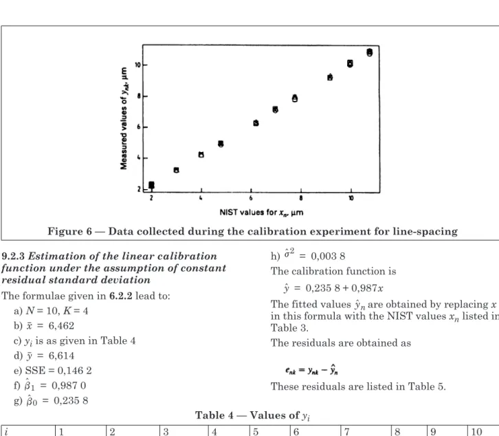
The residuals plot (Figure 8) shows that replicate 2 has consistently lower residual values than the other replicates. These low residual values can be traced back to the original data in Table 3 , which are consistently lower for iteration 2 than for the other iterations. No definite explanation was found for this phenomenon, and the data from replicate 2 were retained as representative of the measurement system's behavior under normal operating conditions. This suggestion is confirmed by Figure 9, which shows the plot of the standard deviation of the repeated measurements of RM against the accepted values of that RM.

Estimate the calibration function under the assumption of proportional residual standard deviation and plot the calibration function and the residuals. The fitted values, , are obtained by replacing xi this formula with the NIST values xn. These fitted values are given in Table 7. Figure 10 supports the assumption of linearity in the same way as in Figure 7. The coefficients of the linear calibration function have changed slightly compared to those in Figure 7. This change is the result of assigning less weight to the measured values for large line spacings than to the measured values for small line spacings (proportional residual standard deviation assumption).

The ANOVA table reveals that the variability in the residuals due to lack of fit ( ) is less than the variability in the data due to pure error ( ). The ratio is less than the F0.95 value (8.30) equal to 2.27. This confirms that the linearity assumption is appropriate for the calibration. experiment described in this example.

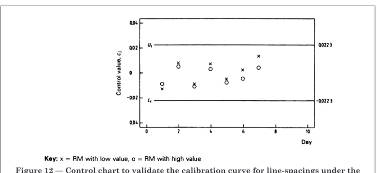
Control method

Since only two RMs are used in the control chart, all control values are included in the calculation of an estimate of the coefficient of variation of a.

Annex A (normative)

List of symbols and abbreviations

Annex B (normative)

Basic method when the number of replicates is not constant

Annex C (informative) Bibliography